Software Environments

Figure 5-1 shows an example of software environment tiers. There are four tiers—DEV, TEST, STAGING, and PROD—where code is progressively deployed as it passes through additional levels of testing and verification until ultimately being released to the production environment (PROD). To get a sense of how code moves through various tiers, let’s take a look at an example process for testing and promoting code.

The promotion process typically starts with a merge request. When you create a merge request, a continuous integration (CI) pipeline runs unit tests as a first check of code functionality. If these tests pass, the code can be merged.

Once the code is blessed by your merge request reviewer and is committed, it gets deployed to a DEV environment. The DEV environment can be used for running integration tests, where you validate that the code operates as expected while connecting to databases, APIs, and any other required services. Once your integration tests are passing, the code would then be promoted to a TEST environment. Code that makes it to the TEST environment is stable enough for quality assurance (QA) testing.

When you’re satisfied with the QA results, it’s time to create a new release candidate. The code is moved from the TEST environment to STAGING, where it can run for an additional time period before being deployed to PROD.

Figure 5-1. Example development environments

This practice of progressively evaluating a system before releasing code updates to end users helps build quality into the development process.

Data Environments

The same environment system is also present when developing data logic. One of the projects I worked on was an analytics platform where we ingested and surfaced data to third-party analysts. Similar to the code promotion process in Figure 5-1, the analysts wanted different tiers of data environments to test their queries. This included a development tier, which contained a small amount of sample data, a test tier with a larger sample of data, a validation tier with a copy of production data, and finally a production tier.

You can see this process in Figure 5-2. Initially when the analysts were figuring out their queries, they worked against a small dataset in DEV. This allowed them to easily verify the query results by hand. When they were satisfied with the initial designs, the analysts promoted the queries to TEST, where a larger dataset was available to test and refine the queries.

Figure 5-2. Example data environments

In the same way that code has to move through multiple levels of testing and QA before release, the analytical queries had to follow the same process on the data side. The analysts were creating reports that would be used to drive policy decisions by the US government, so it was essential to ensure that the queries surfaced the exact data that was expected. Because of this, the data in VALIDATION was the same as the data in PROD. This gave the analysts an exact comparison to validate the results they got when running queries in PROD.

Data Pipeline Environments

Data pipelines benefit from a hybrid of software development and data environments, enabling you to progressively test code updates and data processing fidelity.¹ Figure 5-3 shows an example hybrid environment where the VALIDATION environment in Figure 5-2 maps to the STAGING environment.

Figure 5-3. Environments for data pipeline design

As code is promoted to higher environments (i.e., closer to PROD), it runs against progressively more data. In Chapter 7 you’ll learn specifics about data pipeline testing, but for now it’s sufficient to think about validating pipeline operation at a high level.

Similar to the analysts, you first want to make sure the pipeline runs well against a small set of data. Typically you don’t just run the pipeline in DEV and TEST; you would also validate that the results are what you expect.

In STAGING, it’s best to use data that is as close as possible to your production data, although this may not be possible because of limited resources, customer agreements, or regulations. In the analytical platform I mentioned earlier, we could not run PROD data using our STAGING pipelines due to government security regulations. By testing with full-scale PROD-like data, you can have high confidence that pipeline updates will work as expected when you deploy them to PROD.

In addition to running pipelines against PROD-like data, a STAGING environment gives you a place to let the pipeline run for a longer time period before a release. For example, if you are expanding from running a single pipeline job to several in parallel, a STAGING environment can let you run these pipelines concurrently over a few days to assess performance issues that are harder to pin down (e.g., resource contention) before releasing the update to PROD.

Environment Planning

With dual requirements to support software development and data environments, it’s important to think about what you will need to support both data pipeline testing and data consumers.

Without considering this up front, you can end up being painted into a corner. Figure 5-4 depicts the environment design for the analytical platform I mentioned earlier, where our team had insufficient development and data environments.

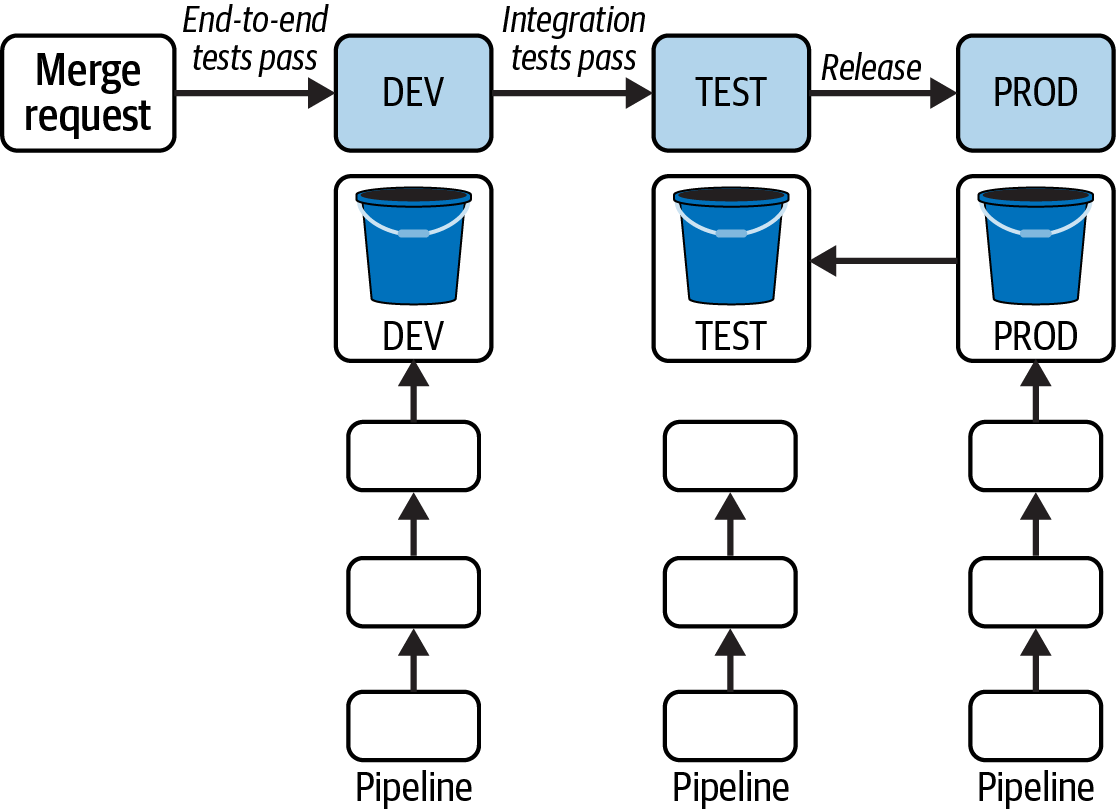
Figure 5-4. Implications of inadequate environments

This design began with three environments. The team had two uses for the DEV environment. One was to deploy merged code for further testing, as in Figure 5-1. We also used DEV to test branches, giving us an opportunity to try out changes before initiating a merge request. TEST was used as both the test and staging environment, and PROD was used for production.

Initially we ran the pipelines in each tier. The input data came from another pipeline owned by a different team, so we could use the data from their TEST environment to run our pipelines. Things became problematic when the analysts requested that TEST data be a copy of PROD, depicted in Figure 5-4 with the arrow going from the PROD bucket to TEST.

With PROD data synced to TEST, these environments became coupled. Our team could no longer run the TEST pipeline, as the data would overwrite the PROD copy. Instead of making the changes necessary to continue having a TEST environment, the decision was made to stop running the pipeline in TEST.

As a result, the only full pipeline tests we could run before a release used the small sample dataset in DEV. When bugs inevitably occurred with medium- to large-scale data in production, the analysts lost trust in the system, no longer believing it to be accurate or reliable.

Containers

One approach for ensuring a consistent and repeatable development environment is to use containers. Containers bundle code and dependencies into a single package that can run anywhere. This means code runs in the same environment whether you are developing locally or running in production, which helps alleviate problems arising from differences between how you develop code and how it behaves when deployed.

Containers have become popular in large part due to the work of Docker, both in its product offerings and in its work on the Open Container Initiative, which develops standards for containerization. I’ll be using Docker examples throughout the rest of this chapter to illustrate working with containers.

To get a sense of the importance of having a consistent development environment, imagine if you were working on a data transformation job running in Spark. Without containers, you might approach local development by installing Spark and its dependencies locally. Perhaps after a few months, another developer starts working in Spark and downloads a newer version. In the meantime, your production environment is pegged to a specific Spark version because of a dependency needed by data consumers running Spark queries. You now have three different versions of a dependency across development and production environments. This can result in code behaving differently in each environment in ways that can be difficult to reproduce and investigate to determine the root cause of the differences.

I’ve seen a case of this where a developer was working on some code that used a new feature of a database we were running. We had a production image of the database, but because this wasn’t used in the development environment, the developer did not realize the new feature was not available in our production version. In the end, we had to scrap the work.

Container lifecycle

While it is true that using containers helps create a consistent, repeatable development process, the realities of the container lifecycle can spoil this claim in practice.

Docker containers and images can be like bad houseguests. Once you invite them in, they won’t leave until you force them out. In my experience, this tends to be the primary culprit of mismatches between containerized environments. It makes me sad just thinking about the amount of time I’ve spent with colleagues trying to figure out the “it works on my machine” issue, only to realize one of us is running an out-of-date container.

To get a sense of how this can happen, let’s take a look at the lifecycle of a container. Containers are created from images. An image can be specified as a link to a prebuilt image in a repository, or by specifying a Dockerfile that will be built to create an image. In both cases, the first thing Docker does when it creates a container is to see whether the desired image is present in the local repository on your machine. If it isn’t, it pulls or creates the image, adding it to your local repository.

Let’s consider what happens over time. Figure 5-5 shows a view over time of running a container from the Postgres image tagged latest.

Figure 5-5. Container lifecycle showing how an image with a latest tag may not truly be the latest version of the image

At the top of Figure 5-5, the official Postgres Docker repository is shown, where the latest tag is periodically updated with the most recent stable Postgres version. At T0, a container is created by issuing a run command for the image postgres:latest. Because there is no image for postgres:latest in the local Docker image repo, the current latest tagged image is pulled from the Postgres Docker repo. The container runs for a while before it is destroyed when it is no longer needed.

Sometime later at T1, you need to run Postgres again, so you issue the same run command, but because a postgres:latest image is already in your local repository, Docker will create a container based on the image that was downloaded at T0. This image is no longer the latest, as there have been two updates to the postgres:latest image in the Postgres Docker repo since T0.

This is exactly how Docker is expected to operate, but it’s very easy to forget that you could be running old containers and/or old images. For this reason, it’s important to get into the practice of regularly deleting and re-creating your images and containers.

Much like you may pin a code library or module to a specific version to prevent unexpected breakages when the “latest” version changes, using specific versions of Docker images works in the same way. In both cases, you have to navigate the trade-off of using the most recent, up-to-date versions of a dependency versus an upgrade process, where pinned versions need to be monitored and evaluated for updates.

When working with containers that use images, use docker pull to download a new image, and then re-create the container. If you’re using a Dockerfile to build an image, running docker build —no-cache will rebuild the image without relying on any existing layers, guaranteeing that you are rebuilding from scratch. If you’re using docker-compose, which you’ll see more about in this chapter, you can specify “pull_policy: always” in the service definition to always get the most up-to-date image.

When in doubt, you can always inspect the images and containers to check creation timestamps. For example, let’s say you want to see what Postgres images you have locally:

$ docker images
REPOSITORY            TAG       IMAGE ID       CREATED        SIZE
postgres              latest    f8dd270e5152   8 days ago     376MB
postgres              11.1      5a02f920193b   3 years ago    312MB

To determine what images a container is running, you can first list the containers, using -a to show stopped containers. It’s important to check for stopped containers so that you’re aware of containers that could be restarted instead of re-created:

$ docker container ls -a
CONTAINER ID  IMAGE           CREATED          STATUS               
2007866a1f6c  postgres        48 minutes ago   Up 48 minutes               
7eea49adaae4  postgres:11.1   2 hours ago      Exited (0) 2 hours ago

You can see the name of the image in the container ls output. To get more detailed information on the image used for the container, you can run docker inspect. In this case, you can see that the latest Postgres image was created on August 12, 2022:

$ docker image inspect postgres
"RepoTags": [
           "postgres:latest"
      ],
      ...
      "Created": "2022-08-12T00:44:14.711354701Z",

In addition to keeping your containers up to date, regularly running docker prune on volumes, containers, and images will help minimize the resources Docker is taking up on your local machine.

Container composition

With multiple services to set up for data pipeline development, bringing together multiple containers can be necessary. This functionality is provided by Docker Compose.

As an example, consider the streaming pipeline shown in Figure 5-6.

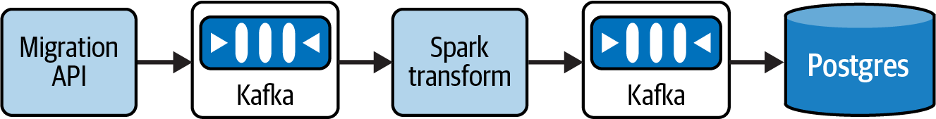
Figure 5-6. Bird migration tracking pipeline

The pipeline in Figure 5-6 is part of another offering from HoD: migration tracking. Researchers studying bird migration habitats have tagged birds with tracking devices that are picked up by towers near popular migration sites. To study the impacts of habitat destruction, the researchers want to collect and analyze information about the birds coming back to these sites on a yearly basis.

When a bird flies near a tower, the tracking information is registered and published to the Migration API. This data is captured by Kafka and streamed to a Spark transformation stage, the result of which is streamed into a Postgres database.

With this architecture in mind, let’s take a look at how to build a Docker Compose environment. Rather than focusing on the syntax, in this section you’ll learn how to approach the design of Compose files. If you are interested in learning more about Docker Compose, check out the Compose file specification.

The Docker Compose files in the GitHub repo for this book are not intended to be run, but rather are provided as high-level examples. If you’d like to try applying these techniques in a live Docker Compose setting, you can check out the Compose examples provided by Docker.

At a high level, the Docker Compose file for the pipeline in Figure 5-6 would include services for Kafka, Postgres, and the data transformation. Each service entry creates a new container, as shown in the following code sample (the full Compose file can be found in transform-docker-compose.yml):

services:
 kafka:
   image: confluentinc/cp-kafka:7.2.1
   . . .

 postgres:
   image: postgres:latest
   . . .

 transform:
   image: image/repo/transform_image:latest
   . . .

networks:
 migration:

In the preceding code, networks identifies which services can talk to one another in a Docker Compose environment. It’s omitted from the high-level view, but every service is on the migration network. This ensures that transform can publish to kafka and postgres can read from kafka.

Running local code against production dependencies

Let’s start by taking a look at the transform container definition:

 transform:
   image: container/repo/transform_image:latest
   container_name: transform
   environment:
     KAFKA_TOPIC_READ: migration_data
     KAFKA_TOPIC_WRITE: transformed_data
   volumes:
    - ./code_root/transform:/container_code/path
   networks:
    migration:

The image is built from the transformation code and stored in the HoD image registry. This is the same image that runs in production. The environment variables KAFKA_TOPIC_READ and KAFKA_TOPIC_WRITE are used by the Spark job to determine which Kafka topics to read from and write to.

To test local code changes there is a volume mounted to the directory where the local transformation code resides, ./code_root/transform, mapping it to the expected location within the container for the Spark job, /container_code/path.

Using a production image and mounting your local code gives you the ability to modify code while still using the environment in which the code runs in production. If you need to upgrade or add new libraries, you need to either build the image with those new dependencies or create a Dockerfile for development that adds the dependencies to the existing image:

FROM container/repo/transform_image:latest

WORKDIR /
COPY requirements.txt requirements.txt
RUN pip install -r requirements.txt

To use the Dockerfile with the new dependencies instead of the original image, you would update the transform container to build from the Dockerfile:

transform:
   build: Dockerfile
   container_name: transform

This is a bit more involved than if you were developing locally without containers, where you could just install a new library and move on. This has the advantage of making dependency modification more explicit to a developer. If you’re working with Python, as in this example, it can be a helpful reminder to make sure you keep requirements files updated.

Using environment variables

Taking a look at the postgres container definition, there is also a volume defined—this is for a location for Postgres to save data to. The POSTGRES_USER and POSTGRES_PASSWORD values are set based on the environment the Compose file is run in, using the environment variables PG_USER and PG_DATA:

 postgres:
   image: postgres
   container_name: postgres
   environment:
     POSTGRES_USER: ${PG_USER}
     POSTGRES_PASSWORD: ${PG_PASS}
   volumes:
     - pg_data:/var/lib/postgresql/data
   networks:
     - migration

Using environment variables encourages good practices, such as not hardcoding credential information into Compose files. To keep your local environment clean, you can use a .env file to define the environment variables needed for Docker Compose.

Sharing configurations

When you have services that are reused across different Compose files, you can consolidate them into a single shared file. This is a good practice for keeping shared resources consistently defined across teams.

To see shared configurations in action, let’s look at an additional dependency for the transformation process in Figure 5-6. Part of the transformation process involves acquiring bird species information from a species table in the Postgres database. This is provided by an API developed by another team. Figure 5-7 shows the API layer added to the migration tracking pipeline.

Figure 5-7. Bird migration tracking pipeline with API dependency

There are now two different teams that will use the postgres container and the api container for development. In scenarios like this, it is helpful to share Compose configurations. Consider the Compose file for API development, which you can find at api-docker-compose.yml:

services:
 postgres:
   image: postgres
   . . .    

 api:
   image: container/repo/api_image:latest
   container_name: api
   environment:
     POSTGRES_USER: ${PG_USER}
     POSTGRES_PASSWORD: ${PG_PASS}
     POSTGRES_PORT: ${PG_PORT}
     POSTGRES_HOST: ${PG_HOST}
   volumes:
    - ./code_root/api:/container_code/path
   networks:
    migration:
   depends_on:
    - postgres

This uses the same Postgres service as the transform Compose file, and an API service with a local mount for development. Notice that the API service needs the Postgres credentials so that it can access the database.

For the transformer environment, you would need to add the api container to access the species information while developing the transformer, which you can find at transform-docker-compose.yml:

services:
 kafka:
   image: confluentinc/cp-kafka:7.2.1
   . . .

 postgres:
   image: postgres:12.12
   . . .

 transform:
   image: image/repo/transform_image:latest
   . . .

 api:
   image: container/repo/api_image:latest
   environment:
     POSTGRES_USER: ${PG_USER}
     . . .

In this situation, you have repeated configurations for the API and Postgres services, which can easily get out of sync. Let’s take a look at how to share configurations to minimize this overlap.

First, you can create a Compose file that contains the shared resources, such as in the following dev-docker-compose.yml. For the postgres container, you can share pretty much the entire service definition. The network is also shared, so you can include that here as well:

services:

 postgres:
   image: postgres
   environment:
     POSTGRES_USER: ${PG_USER}
     POSTGRES_PASSWORD: ${PG_PASS}
   volumes:
     - pg_data:/var/lib/postgresql/data
   networks:
     - migration    

volumes:
 pg_data:
   name: postgres

networks:
 migration:

For the API service, you would want to share the environment but leave the image setting to the developers (you’ll see why in the next section):

api:
   environment:
     POSTGRES_USER: ${PG_USER}
     POSTGRES_PASSWORD: ${PG_PASS}
     POSTGRES_PORT: ${PG_PORT}
     POSTGRES_HOST: ${PG_HOST}
   networks:
    migration:
   depends_on:
    - postgres

With the common setup shown in the preceding code, the next step is to create new transform and API Compose files. These will be fairly minimal now, as a lot of the setup is in the shared file.

The API Compose file, api-docker-compose.yml, contains only the following lines; the rest will be supplied by the shared file. Note that the image tag has changed here to convey that the API team might be working against a different image than the transform team as well as mounting local code:

services:  
 api:
   image: container/repo/api_image:dev_tag
   container_name: api
   volumes:
    - ./code_root/api:/container_code/path

Because the api container in the shared file includes the depends_on clause for Postgres, you don’t need to explicitly add the Postgres service in the API Compose file.

For the transform Compose file, transform-docker-compose.yml, the kafka and transformer sections are the same. The primary difference is that the Postgres service is removed and the API service definition is minimal. Note that the transformer team is using the latest image tag for the API service and there is no local code mounted:

services:
 kafka:
   . . .

 transform:
   . . .

 api:
   image: container/repo/api_image:latest
   container_name: api

Note

Sharing Compose configurations is an important practice for teams that work on shared elements, such as the Postgres database in this example.

This example is inspired by a scenario where two teams were developing against, ostensibly, the same database container but were using slightly different settings in the Compose files. It eventually became clear that the different configurations weren’t compatible and that the database creation wasn’t accurate for one of the teams. Moving to a shared configuration alleviated this issue.

Now that you have a common Compose file and the reduced transform and API Compose files, you can start the containers.

For the transform containers:

docker compose -f transform-docker-compose.yml -f dev-compose-file.yml up

For the api containers:

docker compose -f api-docker-compose.yml -f dev-compose-file.yml up

The order in which you specify the Compose files is important: the last file you apply will override values specified in earlier files. This is why the image was not included in the API service definition in dev-compose-file; it would have forced the same image to be used for both API and transformer development.

Consolidating common settings

In the previous example, you learned how to share container configurations across multiple Compose files. Another way you can reduce redundancy is by using extension fields to share common variables within a Compose file.

Looking at the shared dev-docker-compose.yml from the previous section, the PG_USER and PG_PASS environment variables are referenced by both the api and postgres containers. To set these in a single place, you can create an extension field, as this snippet from dev-docker-compose.yml shows:

x-environ: &def-common
 environment:
   &common-env
   POSTGRES_USER: ${PG_USER}
   POSTGRES_PASSWORD: ${PG_PASS}

services:
 postgres:
   image: postgres
   environment
     <<: *common-env
     . . .

 api:
     environment:
       <<: *common-env
       POSTGRES_PORT: ${PG_PORT}
       POSTGRES_HOST: ${PG_HOST}
     . . .

The extension field, x-environ, contains the shared environment variables in the common-env anchor. For the Postgres service, we only need the USER and PASS variables, but you can see how common-env can be used as a supplemental value for the api container, where you also want to define the PORT and HOST.

Resource Dependency Reduction

You’ve now got some good tools for creating a reproducible, consistent development environment with the Docker techniques from the previous section. There’s a good chance you will have to interact with dependencies outside your local environment. You’ll see a lot more on this topic in Part III.

Reducing the external dependencies you interact with will help you reduce costs and speed up development. To understand why, let’s revisit the ephemeral environment setup I described earlier, pictured in Figure 5-8. I’ve split the environment into two sections, the portion that ran locally and the portion that ran in the cloud.

Figure 5-8. Ephemeral development environment setup

Before launching the pipeline job, a small sample dataset was copied to cloud storage. To initiate a job, a message was submitted to the cloud queue, most often using the corresponding cloud UI. The scheduler ran locally, extracting the job information from the message and launching the pipeline to run in a cluster. At the end of the job, the result was written to cloud storage, which backed a Hive metastore. The metastore definition was created in an RDS instance. Once the metastore was updated, the cluster terminated, sending a response back to the local environment.

Notice that a lot of cloud resources are being created to run a small amount of sample data. In addition to the associated cloud costs, I found debugging to be much more involved versus running locally in containers. For one thing, if the environment creation script failed to create all the resources, I had to figure out what went wrong and sometimes delete individual services by hand. For another, when you are running services in containers locally, you have access to logs that can be hard to find and access in the cloud, if they are created at all.

Remember the capacity issue I mentioned in Chapter 2? That could happen here as well. Without capacity to run the cluster, you couldn’t run a pipeline test.

The environment in Figure 5-8 is a pretty extreme example of running cloud services as part of a development environment. In a lot of cases, you can limit the cloud resource overhead, particularly if you are using containerization and good coding practices. You’ll see advice on coding practices in Chapter 6 and learn how to reduce dependencies on cloud services in Part III.

In some cases, you may need to connect to external services as part of local development. For example, I worked on an analysis pipeline that sourced data from the results of an internal ingestion process. We had the internal ingestion running in a test environment, populating the source database for the analysis pipeline. I connected to this source database while working on the analysis pipeline. Running a large Spark job could be another case where you can’t run locally. In this case, you might need to submit to a cluster to run a job.

A hybrid approach can be a good middle ground, where you build in the capability to run services locally or connect to them. I did this when augmenting a pipeline to add functionality to write part of the transformed data to cloud storage. At first, I simply needed to validate that the correct data was getting saved, something I could do by writing to a temp file and examining the results. For the portion of the work where I was designing the cloud storage interface, I connected to cloud storage because I needed to ensure that the interactions between the code and the cloud APIs were working as intended.

This approach both expedited development by not having to take an extra step to download the new object from the cloud to inspect the results, and minimized object interaction events and the associated costs. On top of this, the ability to write the file locally was useful for running unit tests.

You can also use a hybrid approach like this with some managed cloud services. For example, let’s say the Postgres database in Figure 5-6 was hosted in Google Cloud SQL. You could use a local Postgres container for development instead of connecting to Cloud SQL by providing an alternative set of database credentials for local development.

Resource Cleanup

One task that’s often cited in cost-cutting initiatives is cleaning up idle and unused resources. These resources can accumulate in the development and testing process if you don’t take specific steps to clean them up after you are finished using them.

If you’re creating clusters as part of your development process, setting auto-termination will ensure that these resources are cleaned up after a period of inactivity, such as with auto-termination for EMR clusters. Similarly, using autoscaling on development resources to reduce capacity in quiescent times will also help save costs. For example, you can set pod autoscaling in Kubernetes to scale down when not in use.

You can also take advantage of idle resource monitoring to find and terminate resources that are no longer in use. This is provided for free² for Google Compute Engine.

Many cloud databases also have scaling settings, such as reducing read and write capacity for DynamoDB and scaling down RDS. This lets you limit resource consumption when these services aren’t being used.

Even in cases where resources should get cleaned up, you may need to add some extra guardrails. The ephemeral environments I mentioned had a teardown script, but due to some entangled security permissions, they didn’t always tear down entirely. Every so often, someone would audit the existing “ephemeral” environments and harangue developers to shut them down, if they could even figure out who was responsible for creating them in the first place.

You can use labels and tags on your cloud resources to identify them as development related and eligible for automatic cleanup. This is especially useful for automated cleanup scripts that look for orphaned or idle resources. On one project, we had a job that looked for EMR clusters that were older than a certain number of days and terminated them. Keep in mind that you pay for partial hours, startup time, and teardown time, so don’t be overaggressive with termination.