
Numbers Tutorial
Whether you’re new(ish) to Numbers, or to spreadsheets in general, this is for you. It’s a “just dive in” exercise that introduces you to many of Numbers’ features and interface elements, and demonstrates different ways of achieving the same goal. You’ll also see how they work together—something the rest of this book can’t always describe, as it must cover features separately in order to include their details.
I used many guinea pigs (none were harmed) in developing this tour: male and female, ages 13 to 60-something, spreadsheet neophytes to Numbers dabblers to experienced Excel users. Everybody learned something—often things they wouldn’t have thought to explore on their own.
Table Terminology
In case you come to this section without the most basic knowledge Numbers’ interface, here’s an overview of what you absolutely need to know about tables.
The basic parts of a table are shown in Figure 188.

Some components of a table aren’t available unless the table is either selected or active. When any cell in a table is selected, the table is active: the Row bar and the Column bar, and all four corner handles appear. Labels in the Row and Column bars turn blue when they contain selected cells.
If you click the Table ![]() handle, all the cells are deselected and the table changes from its active state to the selected state. The Row/Column handle in the table’s lower-right corner disappears, and square white selection handles appear at that corner and in the midpoints of the right and bottom edges. If you click outside the table—that is, on the sheet—the table becomes inactive, and all its controls disappear (Figure 189).
handle, all the cells are deselected and the table changes from its active state to the selected state. The Row/Column handle in the table’s lower-right corner disappears, and square white selection handles appear at that corner and in the midpoints of the right and bottom edges. If you click outside the table—that is, on the sheet—the table becomes inactive, and all its controls disappear (Figure 189).

The Tutorial
Get Started
Set some preferences:
Whether the figures in this tutorial match what’s on your screen depends, in many cases, upon your settings in Numbers’ Preferences, so let’s start with that. Choose Numbers > Preferences > General, and make sure these settings are on:
- For New Documents: Show Template Chooser
- Editing: Show Suggestions When Editing Table Cells
- Cell References: Use Header Names as Labels
Start with a new document and table:
Choose File > New, and double-click the Blank template in the Choose a Template window.
Set Up the Table
Hide the table’s name:
A new table defaults to the name Table 1 (or whatever consecutive number needed to differentiate it from other tables on the sheet). Instead of renaming the table, let’s just hide its name from view, using the Format Inspector:
- If the table is neither active nor selected (see Table Terminology), click anywhere inside it to select it.
- If the Format
 button is not selected in the Toolbar, click it to open the Inspector panel.
 - Click the Table tab at the top of the Inspector panel.
- In the Headers & Footer section, click Table Name to deselect it (Figure 190).

The name disappears from the top of the table, and the table and its Column bar shift up to close the gap.
Cut the table down to size:
Your table needs to start with ten rows and five columns:
- Grab the Row
 handle at the bottom-left corner and drag it upward until only 10 rows are left.
 - Drag the Column
 handle at the upper right of the table inward until you have only columns A to E left.
If you overshoot your goal, drag the handle in the opposite direction to restore some rows or columns.
Enter a Formula
- Click in cell
B2(it may already be selected, since it’s the first non-header cell) and type the equals sign to signify a formula. The formula editor pops open (Figure 191).
Figure 191: Click the cell to select it and type an equals sign to open the formula editor. - Type
ran. As you type what Numbers assumes to be a function (a pre-defined formula), it’s placed inside a token—a lozenge that’s easily selected and manipulated in the formula editor. In the meantime, Numbers guesses what function you want so you don’t have to type the entire name; the suggestions appear in a bar beneath the formula editor (Figure 192).
Figure 192: Numbers watches what you type and suggests functions that match what you’ve typed so far. - Click RANDBETWEEN because we want a random number that falls between two extremes we’ll specify.
More tokens appear in the formula editor, labeled with their purpose. Functions need information (numbers or text) to work with; these are called the function’s arguments. They go in parentheses after the function name, with commas between multiple arguments. In the formula editor, the “parentheses” are formed by the function token on one side (its curved shape suggests an open parentheses) and a chunky curve on the other. The tokens show which arguments a function needs. RANDBETWEEN needs to know the lower and upper limits of the range of numbers it should supply (Figure 193).

Figure 193: The function name is embedded in a token that serves as the open parenthesis. The loweranduppertokens describe the information RANDBETWEEN needs to generate random numbers. - The
lowertoken is slightly darkened, to show that it’s selected; type25to replace it (typing replaces selected text). Click theuppertoken, or tab to it, and type200(Figure 194).
Figure 194: Replace the tokens with numbers. - Click the Accept
 button, or press Return or Enter, to enter your formula, and you see the number it generates (Figure 195).

Edit a Formula Argument
- If cell
B2is selected, click it to reopen the formula editor; otherwise, double-click it. - Change 200 to 250, editing the number inside the editor the way you would in a word processor (Figure 196).

Figure 196: Select the second parameter and change it to 250. - Press Command-Return to close the editor and remain in
B2.
Use Autofill to Fill Cells
Autofill saves you lots of time by filling cells for you based on either an initial pattern or a starting formula:
- With
B2still selected (if it doesn’t have a blue frame around it, click to select it), move your pointer towards the bottom, center of the cell until you see the yellow autofill handle. - Drag the handle down to
B6so that you have five cells selected, as shown in Figure 197. (A range of cells is referred to by its first and last cell, so this selection isB2:B6.)
Figure 197: Left: A selected cell and its autofill handle. Right: The autofilled cells. - Note that the Quick Calculation bar (I call it the Quick Calc bar) at the bottom of the window (Figure 198) shows some statistics about the selected cells, such as their sum and average.

Figure 198: The Quick Calc bar displays statistics about the selected cells. - Autofill the formula across three columns:
- With
B2:B6still selected (if it’s not, just drag across those cells), move your pointer to the middle of the right edge of the selection until the yellow autofill handle appears. - Drag the handle to the right, through column D.
- With
Now you have a 3-by-5 block of cells—B2:D6—with numbers in them, as in Figure 199.

Get Some Statistics
Sum the columns using the Function menu:
With the block B2:D6 selected, click the Formula ![]() button in the toolbar, and choose Sum from its drop-down menu.
button in the toolbar, and choose Sum from its drop-down menu.
The sum for each column is entered beneath the numbers, in row 7—whose filled-in cells are now selected—because Numbers reasonably assumes that’s where you want the totals (Figure 200).

Bold the totals:
With B7:D7 (the sums) still selected, press Command-B to bold the contents of those cells.
Average a row with a Quick Calc token:
- Click in
B2—the upper-left cell in the block of numbers—to select it, and then expand the selection by dragging the white selection handle in its lower-right corner to include the three cells in the first row of numbers,B2:D2(Figure 201).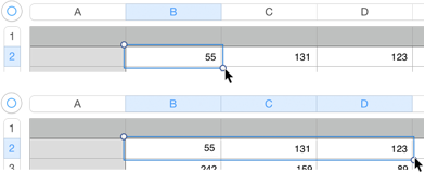
Figure 201: Drag the selection handle from the first cell through to column D. - Drag the AVERAGE token from the Quick Calc bar at the bottom of the table into cell
E2(Figure 202).

Autofill the AVERAGE function:
With E2 and its AVERAGE formula still selected, drag its yellow autofill handle down through Row 6, stopping before the row that holds the sums (Figure 203).

Bold the averages:
Press Command-B while E2:E6 is still selected, to bold the contents.
Deselect the cells:
Press Command-Return.
Check out the formulas:
- Click
E2(the first of the averages) to see the formula that was entered when you dragged the Quick Calc token to it. You seeAVERAGE(B2:D2)displayed at the bottom of the window. - A second click in the cell—or, if it’s not selected, a double-click—opens the formula editor (Figure 204). It, too, shows the formula, of course, and you can click the Cancel
 button or press Command-Return to close it.

Figure 204: Left: The formula as shown in the Smart Cell View for E2. Right: The formula editor opened fromE2. - Click in
E3and note the formula that was entered there when you autofilled it from the cell above:AVERAGE(B3:D3). An autofilled (or pasted) formula automatically changes the cells it references to make them relative to the cell where you put the formula—this is called relative referencing, or relative cell referencing. So, the averages in column E always refer to the cells in their own rows (Figure 205). In effect, each formula has in mind “Average the three cells to my left,” and then figures out those cells’ names.
Figure 205: The cell references in E3’s autofilled formula were automatically adjusted to refer to the cells in its row. - Note the highlighted cells for formulas. Click in
E2and cellsB2:D2turn blue (Figure 206). That’s because the formula inE2references those cells. And, because they are referenced as a range (B2:D2)in a single token, they are all the same color. If a formula references separate cells or blocks of cells, each gets a different color. The tokens in the formula editor and the Smart Cell View match the colors in the referenced cells, as you can see in the silly formula in Figure 207.

Recalculate the random numbers:
- Click in cell
A1, and press Command-X.You won’t actually cut anything from the empty cell, but this forces Numbers to recalculate every formula in the table, so you see all your random numbers change. The sums and averages, of course, change along with them.
- Continue pressing Command-X until at least one of the averages in column E displays more than two decimal numbers (Figure 208).

Format data to display a single decimal place:
- Select the averages in the last column by dragging across
E2:E6(in either direction). - Click the Format
 button in the window’s toolbar to open the Format Inspector at the right of the window, and click the Cell tab.
 - In the Data Format section at the top of the pane, click the up arrow in the button next to the Decimals field to change Auto to 1.
All the numbers in the selected cells display a single decimal point (even if it’s zero) as you can see in (Figure 209). But only the display of the number has changed; the full number is still stored.

Delete and Add Rows
Delete a row:
Change your 3-by-5 grid of random numbers to a 3-by-4 grid:
- Click in
A1to deselect all your data cells. (This isn’t necessary to the following procedure, but can make it easier to see what’s going on.) - Point to the row 6 label in the Row bar at the left of the table (it doesn’t matter what’s selected in the table).
- A menu arrow appears in the label; click it for the pop-up Row menu, and choose Delete Row from the menu.
You still have a row that’s labeled 6, but it contains the sums that used to be in Row 7 (Figure 210).

Check the effect on a formula:
- Click in
B6, where the sum for column B is displayed. - Check the Smart Cell View at the bottom of the window. Your original formula was
SUM(B2:B6); it has changed toSUM(B2:B5)because one of the data rows disappeared.
Numbers is very smart when it comes to figuring out what you’d want to happen to formulas when you delete or add rows or columns.
Add Labels to the Table
Enter label text:
- Click in
A7and typeTotal(yes, below the row with the sums in them). - Press Return to move down to the next cell and type
Maximum. TypeMinimumandHighest Avgin the next two cells in the column. - Click in
E1(above the row averages) and typeAverage(Figure 211).

Move cells by dragging:
Well, you trusted me when I told you to start those first-column labels in A7, and here’s what you get for it: a technique to move cell contents:
- Drag across
A7:A10to select the four labels in the first column. - Press on any cell in the selection—that is, click but keep your finger down on the trackpad or mouse button—until you see the selected block seem to rise up off the table.
- Drag the selection upward and drop it so that the Total label is in
A6, where it belongs (Figure 212).

Right-align the labels:
- With the four labels you’ve just moved still selected (if they’re not, drag across them to select them), click the Format button in the toolbar to open the Format Inspector.
- Go to the Text pane. Of the two tabs partway down the pane, Style and Layout, Style should be selected; if it isn’t, click it.
- In the Alignment section, click the right-align button.
The labels shift to the right of the cells (Figure 213).

Find a Maximum Value
Open the formula editor:
Click in B7 (next to the Maximum label), and type the equals sign to let Numbers know you’re entering a formula (Figure 214).

Type the function name:
Start by typing m and you see function suggestions (type lowercase letters, and let Numbers take care of capitalization). Don’t click a suggested function name, as you did when you entered the RANDBETWEEN function earlier in this exercise; ignore them and finish typing max (Figure 215). Numbers will know that you’ve finished typing the function name when you type the next character, in the next step.

max.Supply the argument:
- Type
(to start the parentheses pair for the information that the MAX function needs to work on (recall that these are a function’s arguments). The MAX function name turns into the token that serves as the left parenthesis (Figure 216).
Figure 216: The MAX function token is also an opening parenthesis. - You must identify the cell range in which Numbers should look for the maximum number. The range is
B2:B5. TypeB(you can use lowercase for typing cell names, too). Numbers suggests column B, as well as functions that start with B (Figure 217); ignore them.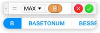
Figure 217: Typing B for a cell reference. - Type
2:(a 2 and a colon) to complete the beginning of the range,B2:. Now the suggestions are not other functions, but the cells you might want for the other end of the range you’re typing.Numbers’ primary assumption is that you want the rest of the occupied cells in row 2, and suggests
E2. However, if you’re using the preference settings described at the beginning of this lesson (in Get Started), Numbers uses the column E header as the column name and suggestsB2:Averageinstead ofB2:E2(Figure 218). Its other suggestions, in the bar beneath the formula editor, are the labeled rows farther down in the column you’re working in, but you don’t need any of these, so continue typing (in the next step).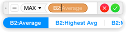
Figure 218: Numbers suggesting various ranges that begin with B2. - Type
B5to finish defining the range (Figure 219). Don’t close the formula editor yet!

Drag a cell-range reference:
Instead of typing a cell range, such as B2:B5, and having to put up with all those suggestions, if the range you want is within easy reach—its cells aren’t scrolled out of the window’s confines, for instance—you can just select them while the formula editor is open instead of typing. (Yes, I hear you: “Now she tells me!”)
- Delete the
B2:B5cell-range token you so painstakingly entered in the formula. (If you closed the formula editor, double-click inB7to reopen it.) If the blinking insertion point is still within the token, press Delete to erase the cell references (the token disappears when you delete the final character); if it’s to the right of the token, a single backspace deletes it. Or, if it’s selected—and you can select it with a click—pressing Delete works for that, too. - With the insertion point blinking in its position just within the parenthesis formed by the MAX token, drag across cells
B2:B5, and the range token appears in the formula editor (Figure 220).

B2:B4 so far; you should continue to include B5.Enter the formula:
Click the Accept ![]() button, or press Command-Return, to close the editor and keep the current cell selected.
button, or press Command-Return, to close the editor and keep the current cell selected.
Edit a Formula
Copy and paste the formula:
We’ll start with the SUM formula and turn it into a MAX formula:
- With
B6(the total for column B) selected, choose Edit > Copy. (Notice thatB2:B5is highlighted because theB6formula refers to those cells.) - Press the Down arrow to move to
B7and choose Edit > Paste. Notice that nowB3:B6is highlighted (Figure 221) becauseB7’s current formula refers to those cells—and that’s a problem, because it’s ignoring the first cell and including the Total figure.

B6 are highlighted. Right: The pasted formula also references the four cells above it, which are not the correct ones.Just as when you use Autofill, described back in Use Autofill to Fill Cells, a copy/paste procedure adjusts the cell references when you put an existing formula in another cell. In this case, Numbers is thinking: “I’m supposed to refer to the four cells immediately above me.” The problem is, of course, that this is not what should happen here. (In addition, it’s still a SUM formula, while the label says Maximum.)
Edit the formula’s cell-range reference:
- With
B7(the first Maximum cell) selected, click in it to open the formula editor; if it’s not selected, double-click to get to the editor. - When the formula editor is open, the highlight for the
B3:B6block in the table gets big handles in its upper-left and lower-right corners. Drag each handle upward to change the beginning and end points of the cell range in the formula (Figure 222).If you can’t reach the lower handle because the formula editor is in the way, move the editor, dragging it by its left edge.

Figure 222: Left: The cell range used by the pasted formula, and the reference in the formula editor. Middle: Drag the upper selection handle upward; the cell reference token changes. Right: Drag the lower handle to finish adjusting the cell range for the formula. - Click Accept
 to close the formula editor.
Now that you’ve adjusted the cell range in a formula by altering both end points (something that works for a selection of any size or shape), I’ll tell you the easy way to do it when you don’t need to change the size of the block, but just position it differently. With the formula editor open and the cell reference token selected, grab the highlighted cells anywhere within the selection—you’ll actually be grabbing the highlight, which you can drag to cover a different block of cells.
Edit the formula’s function:
Since we haven’t yet changed the function in the B7 formula, I get to show you another way to open the formula editor:
- With
B7selected, press Option-Return to open its formula editor. - Double-click the SUM token. The token disappears, and the text SUM is selected. Anything non-token is also turned to text; in this case, it’s the parentheses.
- Type
max, ignoring all of Numbers’ suggestions (Figure 223), and click the Accept button to close the formula editor.

Find a Minimum Value
Use the MIN token:
- Select
B2:B5. - Drag the MIN token from the Quick Calc bar into
B8, next to the Minimum label.
Autofill from multiple cells:
- Drag across
B7andB8—the MIN formula you just entered and the MAX formula you entered previously—to select them both. - With the cells selected, point to their right edge to get the yellow autofill handle, and drag it to the right, through column D.
Numbers copies both the formulas and the formatting through the columns (Figure 224).

Reference only a column in a formula:
This formula is going to find which row has the highest average (the averages are in column E):
- Click in
B9, next to the Highest Avg label. Type an equals sign to open the formula editor, and typemax(. - Instead of specifying the beginning and end of a range, you’re going to tell Numbers to look through an entire column: click on the
Elabel in the Column bar at the top of the table. A token for the column appears in the formula editor; but, as described in Step 3 of Supply the argument:, instead of the column’s name,E, it uses the column’s header label,Average(Figure 225).
Figure 225: Click a column label to use the entire column as the cell reference in a formula. Here, the column header text is being used in the formula instead of the column’s label, the letter E. - Close the formula editor.
- Press Command-B to bold the value in
B9while it’s still selected.
The advantage to using an entire column as the argument for a function is that adding or deleting rows in the table won’t affect the formula.
Apply and Tweak a Paragraph Style
Use a paragraph style to apply multiple formats in one fell swoop:
- Drag across
A6:A9to select the labels you typed, and then Command-click inE1to include the Average label in your selection. (Command-clicking is a standard Mac move to add a non-contiguous item to an existing selection). - Click the Format button in the toolbar if necessary to open the Format Inspector, and go to the Text pane by clicking its tab.
- Click the style name at the top of the pane to open a popover of styles, and choose Label.
Your labels change to white, drop-shadowed text. The text in
A9might wrap down to a second line, making that row deeper than the others in order to accommodate that; we’ll be fixing that shortly. - Press Command-B with the label cells still selected to bold the text for better readability—the Label style stripped out the bold that you had applied previously because it doesn’t include bold formatting (Figure 226).

Figure 226: Select the labels, choose the Label style in the Text pane to apply it to the selection, and restore the bold formatting. - Command-click the Average label in
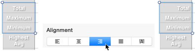
E1to remove it from the selection, and then override the style’s center-aligned format for the other labels by clicking the right-align button in the Alignment section of the pane (Figure 227).
Adjust the Table
Resize the table:
- Click the Table
 handle in the upper-left corner of the table to select the table itself, deselecting all its cells.
 - Drag the square resize handle in the lower-right corner of the table to adjust the row and column sizes without affecting their contents (in this case specifically the text size). Drag up and to the left to make the table smaller (Figure 228). Don’t worry if you scrunch the words in columns A and E, or even the numbers in the rest of the table, since that’s the next thing we’ll attend to. In fact, scrunch away so you can see how to fix that on a column-by-column basis.

Change the width of specific columns:
- In the column bar above the table, drag the divider between A and B to make column A the right size for its labels—especially the long Highest Avg in
A9(Figure 229).
Figure 229: Widen column A to accommodate the Highest Avg label by dragging the column divider. - Drag the divider after column E to accommodate the “Average” label in row 1.
- Select columns B through D (the ones with the random numbers in them) by dragging across their labels in the Column bar.
- Grab a divider to the right of any of the selected labels (that is, not the one before column B) and drag it to the left to narrow all the selected columns at the same time (Figure 230).

Adjust the row heights:
- Select all the rows by dragging across all the labels in the Row bar at the left of the table.
- Drag any interior divider to make the rows taller.
Format cell borders:
- Select the cells with the random numbers in them (
B2:D5) by dragging across them. - Click the Cell tab in the Format Inspector. (If the Format Inspector isn’t open, first click the Format button in the toolbar.)
- In the Border section of the pane, click the All Borders option in the upper-right corner of the grid.
You won’t see much of a change yet because the border lines are so thin.
- Select the dotted line from the second pop-up menu, and set the size to 2 pt (points) by either typing or choosing from the pop-up menu. (If you type, you need only enter the number; “points” is always used as the unit of measure.)
Figure 231 shows what you should have so far.
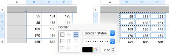
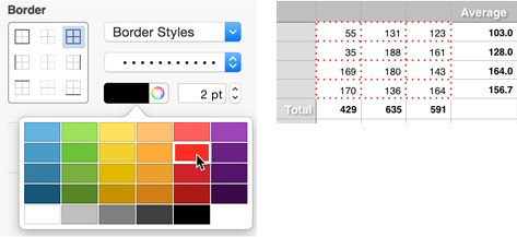
Figure 231: The transformation from plain to… not plain using the Border options in the Cell pane. The dotted borders on the right are surrounded in blue because they’re still selected. - With the borders still selected, choose a color:
- In the Border section of the pane, click the color sample (not the color wheel)—a menu arrow appears as soon as your arrow is within the colored area.
- Click a color in the popover; I’d recommend red, considering how subtle the border is so far if you’ve been using the choices described here.
To see the full effect of your effort, click outside the selected cells or the table to remove the selection frames (Figure 232).
Set Conditional Highlighting for Cells
This is the both the finale and the pièce de résistance. (Sacrè bleu!) The random numbers in the table range from 25 to 250. Format their cells to flag the outliers—the 50 lowest and 50 highest numbers.
Highlight the lowest numbers:
- Select cells
B2:D5again—those with the random numbers—by dragging diagonally across them. - Go to the Format Inspector’s Cell pane.
- Click the Conditional Highlighting button and then click Add a Rule for a popover of choices.
- With Numbers selected at the top of the popover, click Less Than (Figure 233).
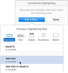
Figure 233: Choose Less Than from the Add a Rule popover. - Type
75in the text field for Rule 1. - Click the Red Fill default choice to get a popover of other choices. As soon as you click it, you see the Red Fill applied to any under-75 cells in your table. Choose Yellow Fill from the popover, and see the random numbers recalculate and yellow applied to those under 75 (Figure 234).

Highlight the highest numbers:
- Click Add a Rule again, and choose Greater Than.
- Enter
200in the field, and choose Teal Fill from the menu beneath it (Figure 235).
Figure 235: This is what you can get with two rules controlling the conditional highlighting. - Click the Done button at the top of the pane to close it.
Watch your random numbers change, and along with them, the totals, averages, and conditional highlights in the cells: click in A1 and repeatedly press Command-X.