
System metrics are a source of valuable information about a system’s state. Alarms and monitors evaluating to a Boolean value indicate the current state and operational context of your systems. Thus, you can take advantage of them to programmatically drive resilience and recoverability, while reducing the complexity of human interaction.
Large-scale systems require regular maintenance operations, such as preventative checks and content updates. These take place during normal system operation and involve removing selected servers from operation. As a result, the system runs at reduced capacity relative to its normal levels and can handle a proportionately smaller load.
Every type of maintenance carries with itself a risk of an outage. However negligible the hazards, they remain real. A minute of downtime at a peak is a lot more costly than the equivalent duration during a trough, and for that reason all maintenance work should be attempted under smallest possible load.
In systems with regular cyclic patterns, peaks and troughs can be clearly distinguished by viewing incoming traffic plots (Figure 5-1). Both extremes of system activity can be assigned to specific hours of the day. It is possible to create an alarm based on the time of day evaluation that goes into alert state during peak. The maintenance processes can be instructed to first consult the alarm state before kicking off their work and to postpone execution when the alert is on. When the demand reaches trough again, the alarm transitions back to a clean state and the processes are given a green light to carry on.

When usage varies in an irregular manner, is unstable, or goes progressively in one direction, the time evaluation rule in the alarm may be replaced by a traffic monitor with a dynamically adjusted threshold, as described by Data-driven thresholds. Such a threshold could be calculated as the p50 of last week’s data points with an additional upper limit set as an appropriate safety value, to avoid capacity reduction when the demand evolves unexpectedly. See Figure 5-1.
In cloud-based settings, this technique can help with autoscaling, or dynamic capacity allocation.
In the same spirit of carrying out work only as resource levels permit, a case could be made for controlling the rate of a staggered system upgrade with the CPU utilization metric.
Suppose you’re dealing with a fleet of servers that is to be upgraded. For the upgrade to complete, every server in the fleet must be taken momentarily out of service. Each such operation immediately puts proportionately more load on the remainder of the fleet. It is assumed that once the server gets upgraded it returns to the fleet on its own, and takes on its due proportion of the load. The task is to complete the upgrade in a reasonable time, but without noticeable performance degradation. The main goal is to avoid excessive load put on too few machines.
It has been established that there will be no noticeable performance degradation as long as the CPU util does not exceed 50% on minutely average. The level of utilization during trough varies, but oscillates at around 30%.
The rate of migration may be controlled with a very simple algorithm as depicted the flowchart in Figure 5-2. The loop continuously checks whether more hosts to be upgraded exist in the fleet. If so, fleet-wide CPU utilization is consulted. If the CPU levels remain within the expected threshold, the fleet can be put under a little more strain by taking another host out for upgrade. Otherwise, the process checks back after some time. The hosts are assumed to automatically rejoin the fleet once they’re done upgrading.

Because CPU util is such a universal system load indicator, this very simple algorithm accounts for a number of scenarios:
The upgrade completes in optimal time keeping within the agreed threshold.
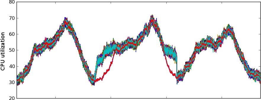
At peak time, when utilization levels rise above 50%, the upgrade process is put on hold to be resumed later when the demand reaches the trough period once again. The process is illustrated in Figure 5-3, showing CPU utilization elevated during before and after the daily peak, relative to baseline levels.
If for some reason the upgraded hosts do get back in service as predicted, the upgrade stops at the agreed CPU level and the operator has more time to remedy the situation.
If during trough the load unexpectedly increases, the CPU util metric will reflect that and the migration will be paused to meet the demand.
Let me bring up one more time a data pipeline example from Chapter 3. Consider a pipeline with three components serially processing a stream of inputs—Loader, Processor, and Collector. For simplicity, I’ll refer to them as A, B, and C. The inputs are submitted by multiple independent sources to component A, which enqueues them for processing in B. Component C fetches inputs from B and processes them at an almost constant rate.
The inputs are processed by C in the order of arrival as retrieved from B’s FIFO queue. The queue serves as an input buffer handling brief input spikes that cannot be handled immediately by C. Whenever the input arrival rate is higher than the departure rate, the queue builds up a backlog. When the arrival rate decreases, the backlog is steadily drained by C.
The three components record their own monitoring metrics with performance information:
Component A records the number of incoming inputs as a flow metric and a percentage of admitted inputs as an availability metric.
Component B records the queue size at any given time—a stock metric with number of elements currently in the buffer.
Component C records the rate of processing as a throughput metric—its average input processing speed expressed in inputs per minute.
The pipeline operates with limited resources to be cost effective, yet there is no limit on how much load can be submitted by each source at any one time. Data pipelines with unpredictable input burstiness should be considered “best effort” and their operational-level agreements must be defined to reflect that. For that reason, an accompanying SLA defines the maximum allowable end-to-end latency to be one hour, but under normal operation a typical turnaround time should not exceed 15 minutes. It also makes clear that it’s better not to admit an input for processing at all than have it breach the SLA latency level.
Suppose the arrival rate has been higher than the departure rate for long enough to accumulate a serious backlog, the clearing of which takes exactly one hour (Figure 5-4). From here on, it makes no sense to admit inputs to the pipeline any faster than the current departure rate, as they will inevitably breach the SLA.

Knowing the speed of processing (departure rate) and maximum latency as defined in the SLA, you can easily calculate the maximum allowable queue size:
Processing rate is recorded by component C. Let’s assume it’s at three items per minute. If the SLA-defined latency is 60 minutes and the C component is capable of processing up to 3 items / min, then the queue may reach up to 180 items before the system fails to meet the SLA.
This way, the throughput metric describing the processing rate from component C can be used to set an admission restriction on component A by calculating the threshold of the queue size in component B.
Fine, but suppose the arrival rate stabilizes at around the maximum allowable queue levels. If arrival rate is equal to departure rate all inputs will meet the SLA just barely, but their end-to-end processing latency will still be very poor. This is not always desirable. If the backlog level is steady for days without any improvement then every client will have a uniformly bad experience. At least two problems exist in this solution:
The clients experiencing poor performance were not necessarily responsible for the build-up, yet they suffer the consequences.
The buffer does not serve its original purpose anymore: it’s unable to capture and deal with occasional, unsustained input bursts as it’s clogged with the backlog and drops all inputs above the maximum queue size.
A further tweaked admission control mechanism could aim at faster recovery to sustainable levels and could look like Figure 5-5.

Suppose that 25% of queue saturation, relative to maximum queue size, would cause an end-to-end latency not exceeding 15 minutes.
Component A accepts all inputs until the queue in component B reaches approximately 25% of the SLA-defined maximum level. At that point component A attempts to drop a percentage of inputs (reflecting relative maximum queue size) for as long as the queue exceeds the limit and not less than the next 4 data points. If the intensity of arrival increases, so does the queue size and so does the percentage of dropped inputs.
This way,
queue saturation is kept below 25%, enforcing a tolerable latency instead of the maximum allowable one hour when the demand exceeds supply
when the sustained uptake in inputs is caused by one or a small group of offending sources, they pay the biggest price in terms of number of dropped items
when the speed of processing by component C changes, max queue size changes its size but the SLA-defined values of one hour and fifteen minutes remain the same
Traditionally, new software rollouts have required constant attention to ensure timely rollback in case things go awry. However, in agile environments that adopt a continuous integration model or in ones with an aggressive deployment schedule, attempting every single rollout with the low possibility of failure by a human operator becomes too costly. The solution is to push out all recent builds automatically. But what if a small, incremental change introduces a critical fault, capable of bringing down the entire system?
To the rescue comes monitoring-enhanced automated rollback.
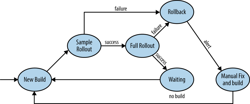
The rollout is divided into two phases that are carried out consecutively. First, a fraction of hosts is separated from the total and used for initial sample deployment of the new software version. The metrics on the remainder of the fleet serve as a baseline for comparison. Performance and availability are measured on both groups of hosts, typically by comparing response times and error rates as well as key user metrics. If performance levels on freshly deployed hosts do not reveal any worrisome signs, a staggered deployment to the remainder of the fleet follows. Otherwise, an automated rollback is initiated to minimize any possible negative impact, the deployment pipeline stops, and the issue is brought to the operator’s attention. The verification may be repeated during the full rollout and after its completion. If the outcome of the deployment is critical, the system immediately reverts to the latest stable version.
The process is modeled on a finite state machine shown in Figure 5-6. In the illustration, the metrics are consulted twice: first after sample rollout and then after completion of all hosts.
While the idea behind the process is a simple one, its practical implementation has a couple of caveats:
The performance comparison must take into account the existence of warm-up effects on the servers getting back into service, and disregard them.
On occasions, false rollbacks may result from unrelated production issues which trick the process into thinking that deployment was at fault.
Sometimes minimal levels of degradation not impacting the users at all may be the reason for pipeline stoppage.
These are all special cases of false positives. Their existence is typically realized early in the process and dealt with accordingly by threshold tuning.
This enhancement of the process connects the best of both worlds: it does not necessitate the operators to be present at all times during numerous software rollouts, while at the same time it keeps any possible negative impact to an absolute minimum.