Figure A-1 illustrates OpenTSDB in its operation. At the core of the solution lies the Timeseries Daemon (TSD), which assists the clients in storing and retrieving metrics from the HBase cluster. The two core components are loosely coupled and can be scaled independently.

Multiple instances of TSDs communicate between three actors: input sources, clients, and the datastore.

Input sources are servers with data collection agents deployed to them. The collectors gather and report hardware statistics, quantitative data extracted from application logs as well as SNMP information reported by the network devices and sensors.

The clients are system operators plotting the charts via the HTTP interface, alerting systems evaluating most recent data points for existence of alertable behavior, and automated processes that use monitoring information as input for routine tasks. TSD’s UI allows for juxtaposing any combination of timeseries at arbitrary temporal granularity starting with one second. The data points may also be exported over HTTP in clear text as inputs to alerting engines and for offline analysis. Such fine granularity is unprecedented at the scale that OpenTSDB can support.

Datastore typically refers to an HBase cluster, although the open source community has reported success with using alternative NoSQL solutions. It should be noted, however, that at the time of this writing HBase is the only supported datastore.

OpenTSDB’s data collection takes place by pushing data to the datastore, that is, the sources report data points to TSD instances with put operations. All put operations are independent in that the reporting servers are not assigned to specific TSDs or the other way around.

Figure A-1. OpenTSDB Architecture, courtesy of Benoît Sigoure

A single-box installation of OpenTSDB can be completed in 15 minutes. It involves deploying an HBase instance and populating it with OpenTSDB schema, spinning up the Timeseries Daemon (TSD), and feeding it with data! OpenTSDB fetches most of its dependencies at build time except for GNUPlot, Java Development Kit (JDK), and HBase. These three need to be installed separately.

To bootstrap a single-node HBase instance, visit this website.

Then for the latest OpenTSDB setup instructions, go here.

Enter the build/ directory in the root of where OpenTSDB was built. It contains the tsdb shellscript wrapper which you’ll use for managing the TSD. Launching a TSD instance requires three mandatory command line options: the TCP port number to use, location of the web root from which to serve static files, and the request cache directory.

Addition of --auto-metric flag gets TSD to create metric entries in TSDB for you on the fly. Otherwise, metrics have to be created with tsdb mkmetric subcommand. While automatic metric creation might not be ideal for a production environment, this very convenient feature saves a lot of typing while playing with tsdb.

The “staticroot” should already be present in the current directory. Create the cache directory and start tsdb on port 4242.

$ ./tsdb tsd --port=4242 --staticroot=./staticroot --cachedir=/tmp/tsd --auto-metric

The last line should read “Ready to serve”. Now go here. You should be greeted by TSD’s HTTP interface. It’s time to upload some data inputs.

A running TSD instance is meant to receive inputs from data collectors in push mode (Figure A-2). The collectors connect to TSD and upload data via clear-text protocol with help of simple put operations. Submitting inputs requires four pieces of information:

Figure A-2. TSD’s HTTP interface

The template for the put directive is as follows:

put <metric> <timestamp> <value> <tagkey=tagvalue> [<tagkey=tagvalue> …]

Every data input must to be described by at least one tag.

To report a data point simply open a TCP connection to a TSD and supply the data as follows:

$ echo "put test.metric $(date +%s) 1 order=first" | nc localhost 4242

$ echo "put test.metric $(date +%s) 2 order=second" | nc localhost 4242

$ echo "put test.metric $(date +%s) 3 order=third" | nc localhost 4242

Now, go back to the HTTP interface and in the metric form field enter “test.metric”. An auto-suggestion helper window should pop up as you type. Leave the tags blank.

Click on the “From” field and when the calendar expands double click the “1m” link. This will set the start time at two minutes ago. Now, click on the “(now)” hyperlink next to the “To” field to select the present time as the end time of the observation. At this point, you should see a plot with three data points.

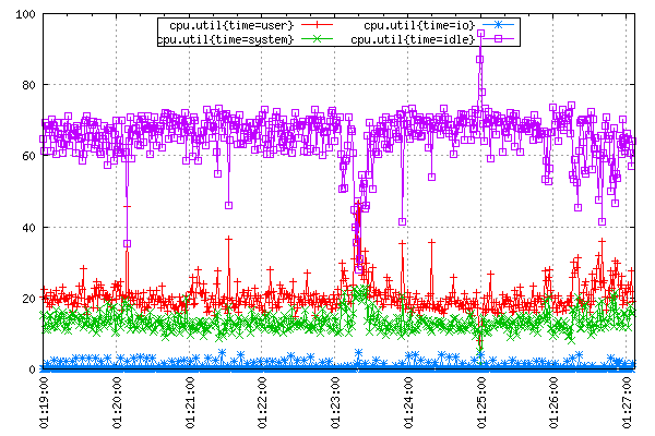
Okay, now let’s report something more useful. Assuming that System Activity Reporter (SAR) is installed on your system, telling it to run with 1 second frequency should result in a fine-grained report of CPU utilization in percentage terms.

$ sar 1

Linux 3.0.0-22-generic (hostname) 14/07/12 _i686_ (2 CPU)

01:18:10 CPU %user %nice %system %iowait %steal %idle

01:18:11 all 18.59 0.00 13.57 2.51 0.00 65.33

01:18:12 all 19.00 0.00 13.00 0.00 0.00 68.00

01:18:13 all 20.81 0.00 11.17 0.00 0.00 68.02

01:18:14 all 17.82 0.00 12.38 0.00 0.00 69.80

…

The following shellscript reads in sar’s output, translates it into TSDB put instructions and uploads them to TSD.

#!/bin/bash
# Ignore sar's header.
sar -u 1 | sed -u -e '1,3d' |
while read time cpu usr nice sys io steal idle; 
do 
    NOW=$(date +%s)

    echo put cpu.util $NOW $usr time=user
    echo put cpu.util $NOW $sys time=system
    echo put cpu.util $NOW $io time=io
    echo put cpu.util $NOW $idle time=idle
    # Report values to standard error.
    echo timestamp:$NOW user:$usr sys:$sys io:$io idle:$idle >&2
done | nc -w 30 localhost 4242

Let it run and pull up the TSD’s HTTP interface in the browser:

Soon enough the resulting plot should look something like the one in Figure A-3.

Figure A-3. Plot of SAR’s CPU utilization

Tagging provides an extremely convenient and flexible mechanism for aggregation by source of data at many levels. Tags are attributes of data inputs that describe their properties and origin. You can think of each tag as an added dimension on your data, with the help of which OpenTSDB will allow you to slice and dice through the data points at will.

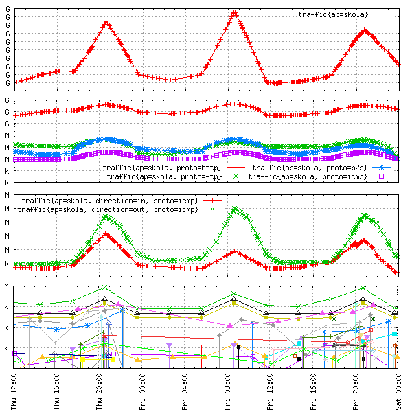
Let me explain the idea on a simple example: network traffic measurement. On a high level, network traffic is a flow of bytes encapsulated in packets. Looking closer, each packet has a source and destination, it represents one or more of the OSI layer protocols, and it has a direction—it either leaves or enters the network. Consider monitoring traffic flow in bytes per interval of time. The put operation for each host would look something like this:

put traffic <time> <value> src=<hostname> subnet=<name> proto=<protocol> direction=<in|out>

Reported traffic data can now be analyzed as cumulative flow, by protocol, by direction, and even by specific source host or any combination of these, for example, incoming HTTP traffic per subnet or outgoing ICMP traffic per host, as illustrated in Figure A-4.

Figure A-4. 72 hours of TCP/IP traffic at different levels of aggregation

Short-lived technical blips that cause cascading failures up and down the solution stack happen in a matter of seconds. OpenTSDB was designed specifically to continuously monitor large clusters of servers at sufficient granularity, empowering the operators to detect and evidence problem sources without having to dig into logs just to extract quantitative information. OpenTSDB records data inputs at one second granularity, which is much finer than the vast majority of monitoring systems can offer.

Having said that, OpenTSDB does not lock the user into data point intervals of specific length. When one second interval is too short to reliably plot the desired effect on a timeseries, it’s possible to select custom temporal input aggregation. In the UI, this is referred to as downsampling. To make the data points on the selected metric’s timeseries less granular, select the “Downsample” checkbox and enter desired interval. The TSD will divide the timeseries into an evenly spaced time period group, aggregate all data inputs reported in that duration, and summarize them with a statistic of choice.

At the time of writing this, the TSD can condense inputs into data points with a selection of summary statistics: min and max—the smallest and largest values per interval (p0 and p100), the sum and average of values, and standard deviation. TSD’s UI refers to summary statistics as aggregators.

Rate of change is a series of data points derived from another timeseries by calculating the difference between two consecutive values from the original series.

Deriving the rate of change is especially useful for counter metrics, which are a special type of stock metric described in detail by Chapter 2. A rate of change of a counter metric is a flow-type metric, describing counter increases per interval.

For all other timeseries, rate of change illustrates the velocity of data point values: speed of their increase or decline, with the latter plotted in negative range. As a result, it usually makes sense to place the rate of change series on the right y-axis, leaving the left side y-axis for series ranging in nonnegative values only.

To plot the rate of change in OpenTSDB check the “Rate” box in the metric options window.

tcollector is written in Python and comes ready-to-run with a number of standard input collectors.

To get it, check out the latest version from the official repository:

$ git clone git://github.com/stumbleupon/tcollector.git

$ cd tcollector

The directory should contain licensing files, base tcollector code and a number of standard input collectors in the collectors/0 subdirectory. If you’ve started your TSD with --auto-metric option, all you need to do now is to start tcollector. The following line will kick off the process with root privileges.

$ sudo TSD_HOST=localhost TCOLLECTOR_PATH=. ./startstop start

Starting ./tcollector.py

Okay, tcollector is running and reporting metrics. After fifteen seconds first inputs should have arrived. Switch back to the HTTP interface and plot some metrics; for example, juxtapose proc.stat.cpu with proc.meminfo.highfree and df.1kblocks.used. A detailed description of each metric’s supported by tcollector can be found here.

For production settings, tcollector should be packaged and deployed system-wide to every monitorable host. Typical setup on each machine involves the following:

It is extremely easy to plug a custom collection agent into tcollector—simply create an executable script or binary that reports data inputs at an interval and place it alongside other agents. The inputs should be printed one per line to standard output in similar format as for the put directive, but with the put directive itself omitted:

<metric> <timestamp> <value> <tagkey=value> [<tagkey=value> …]

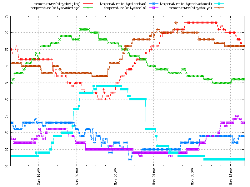
The following agent gathers temperature information for selected cities. It runs continuously in a closed loop at 5 minute intervals.

#!/usr/bin/python
import sys
import time
import urllib2

COLLECTION_INTERVAL = 300
CITIES = ['Beijing', 'Cambridge', 'Farnham', 'Koeln', 'Sebastopol', 'Tokyo']
WEATHER_API = 'http://citytemp.effectivemonitoring.info/get'

def get_temperature(city, scale='c'):
    """Get temperature for a city."""
    city_url = WEATHER_API + '?city=%s&scale=%s' % (city, scale)
    api_response = urllib2.urlopen(city_url).read()
    if api_response.strip().isdigit():
        return eval(api_response)

def main():
    while True:
        for city in CITIES:
            ts = int(time.time())
            city_temp = get_temperature(city, scale='f')
            city_label = city.lower().replace(' ', '_')
            print 'temperature %d %s city=%s' % (ts,  city_temp, city_label)
        sys.stdout.flush()
        time.sleep(COLLECTION_INTERVAL)

if __name__ == "__main__":
    main()

tcollector will always add a host tag to the reported data. This way, data are guaranteed to have at least one dimension, and data points can always be reliably tracked back to a set of machines from which the inputs originated (Figure A-5).

Figure A-5. Data gathered with custom collector

There exist a number of tricks that skillful plotters use to extract the desired effect. Here are just a few of them: