Some people believe that alerting is an art for which proficiency takes long years of trial and error. Perhaps, but most of us can’t wait that long. I prefer to view alerting as an exact science based on logic and probability. It’s about balancing two conflicting objectives: sensitivity, or when to classify an anomaly as problematic, and specificity, or when is it safe to assume that no problem exists. These objectives pull your alerting configuration in two opposite directions. Figuring out the right strategy is not a trivial task, but its effectiveness can be measured. The right choice depends on organizational priorities, the level of recovery built into the monitored system, and the expected impact when things go awry. At any rate, there is nothing supernatural about the process; getting it right is well within everyone’s reach.
In my experience, it’s simply impossible to maintain focused attention on a timeseries in anticipation of a problem. The vast amount of information running through the system generates a great number of timeseries to watch. Hiring people solely for the purpose of watching performance graphs is not very cost effective, and it wouldn’t be a very rewarding job either. Even if it was, though, I’m still not convinced that a human operator would be better at recognizing alertable patterns than a machine.
The process of alerting is full of unstable variables of a qualitative nature, and it presumes an element of responsibility. Priorities are open to interpretation, but the level of severity usually depends on what’s at stake. The extent of pressure involved in incident response varies from organization to organization, but the overall process has a common pattern.
The goal of alerting is to draw operators’ attention to noticeable performance degradation, which manifests itself in three general ways:
Decreased quality of output
Increased response time
Loss of availability
The onus on the operator who receives an alert is to respond to it in a timeframe appropriate to the severity of the degradation. His task is to isolate and identify the source of the problem and mitigate the impact in the shortest time possible. The challenge of balancing sensitivity and specificity is to alert as soon as possible without raising false alarms.
Effective alerting is more than creating alarms and sending notifications. It should facilitate the human response to mechanical faults and drive continuous improvement. To meet these goals, alerting requires a few basic components of IT infrastructure, without which a mature organization simply cannot exist.
First and foremost, you need a monitoring platform that meets a few conditions: it must have a well supported and easily definable way to deploy data gathering agents; it should have a flexible, feature-rich plotting engine that allows for graphing multiple timeseries on a single chart; and it must include an alerting engine that can support sophisticated alarm configurations (tens of thousands of alarms, aggregation, and suppression).
This book does not help you deploy a monitoring platform; I assume you already have one. If you don’t and are wondering which monitoring system best addresses your needs, I recommend making an informed decision by consulting the following Wikipedia article, mentioned earlier in Chapter 1.
A lot of issues result from the fallout of planned production changes. Some of them may be executed automatically, such as a periodic rollout of security patches. Others are manual, like configuration changes carried out by an operator through step-by-step instructions. Maintaining an accurate and complete audit trail—a chronological record of changes in the system—helps in pinpointing cause and effect by letting you correlate aberrant system behavior with the times in the event log. A quick discovery of faults in this way significantly boosts the process of recovery.
An issue tracking system (ITS) helps prioritize reported alerts and thus helps you track the progress of issues as they are being resolved. Tickets coordinate collaboration between resolvers and ensure that the ball does not get dropped, so each and every alert should be recorded in an ITS. With it, the effectiveness of alerting can be reliably measured over time. This helpful side effect of an ITS helps in driving higher standards.
Maintaining a robust alerting configuration starts with realizing the cost of failure and the significance of reacting in time. The cost can be understood and expressed in a variety of ways: time, money, effort, quality, prestige, trust. Each organization can come up with its own definition. The bottom line is that each failure incurs costs corresponding to the extent of the failure’s impact. The first step on the way to effective alerting is to come up with clear range of significance in order to set the priorities right.
Among many failures experienced in a daily system operation, only a fraction deserve an operator’s attention.
Failures are eligible for alerts when their significance is high enough to negatively affect the system’s operation. They are significant if the system will not recover from them by itself. Therefore, the severity of a failure can be considered in terms of two properties: recoverability and impact. Let’s consider those two for a moment.
Recoverability is the potential of a system to restore its state to the prefailure mode without operator intervention. Recoverability can be imagined as a score combining the likelihood of a given failure to go away and the time necessary for its cessation.
Impact is the negative effect on the system’s operation, reflected in the level of resource utilization as well as end user experience. It can be described as an unanticipated cost, which comes in various orders of magnitude. To quote just a few examples for an ecommerce website, from most to least severe:
- Downtime
People can’t buy stuff, leading to loss of immediate revenue as well as potential future customers.
- Partial loss of availability
A fraction of customers won’t spend their money on your site.
- Increased response times
Some users will get impatient and go off to the competition.
- Decrease in content quality
People are less likely to remain on the site and therefore purchase stuff.
- Suboptimal utilization of resources
This uses up money that can potentially be spent better.
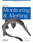
Let’s stagger recoverability and impact into three levels each, as depicted on Figure 3-1, to describe the severity of undesired events. The matrix illustrates a classification of events into nine separate bins, from most to least severe.

Critical
Sudden events with impact so severe as to block user access or severely impair the system’s operation. A failure to prevent critical events increases system downtime and directly translates to unrecoverable losses in productivity or revenue.
Urgent
Events when partial loss of availability is observed, when a fraction of users is unable to get onto the system, or a significant portion of the system becomes unresponsive. These kinds of events require fast intervention to minimize their impact and prevent them from escalating into critical events.
Intervention necessary
Events that require intervention to prevent them from intensifying into critical events. They are not immediately catastrophic, but the system is at a high risk of collapsing without treatment. For instance, the system may build up a backlog that leads to processing delays.
Recoverable
Negative events with relatively noncritical effect on the system, but with the potential to develop into bigger problems if not recovered within an expected timeframe. For instance, the failure of a background map-reduce job may be noncritical to the system’s operation, and no alarm is necessary if a subsequent job succeeds.
Inactionable
A group of events in which a small fraction of users faces transient but serious failures that immediately disappear by themselves. Because of the high speed of recoverability, the inactionable events get resolved before an operator could respond, so it would be ineffective to issue alerts for them. The frequency of these inactionable events should, however, be occasionally verified to ensure that momentary performance degradation remains isolated and negligible.
Automation Tasks
Faults not having an immediate impact on the system’s operation but with a potential of being a supporting factor in other failures.
Early Indicators
Transient events of small to moderate impact affecting a tiny fraction of users. They come as a result of momentary resource saturation and small bugs and may be early indicators of the inability of a system to handle stress.
Optimization Tasks
Events bearing no effect on a system’s functionality but causing inefficiencies in resource utilization that could be eliminated by architectural restructuring or software optimizations.
Nonissues
Anomalies with no perceivable impact, observable as a part of any system operation, particularly at scale.
Only the first four groups require alerting, because only in those cases is the system actually at risk and only then should the operator intervene and alter the system’s state.
For the four alertable groups, the alerting configuration is considered in terms of two contradictory goals: speed and accuracy of detection.
The alerts for critical events should trigger as soon as the initial symptoms of grave failure are present. Critical events require immediate intervention, so it’s okay to trade off reliability of detection for precious time that could be spent on mitigative action. If a few false positives are generated in the process—so be it.
The second group of events, classified as urgent, also necessitate quick intervention, but their relatively higher incidence and lesser severity allow you to wait for additional data points before raising an alarm. The alert is still issued relatively early, but with higher confidence.
System issues for the which operator’s intervention is necessary but does not have to be immediate allows for more liberal data collection times. Effectively, an alert should be issued only when the existence of the problem has been established with a high degree of certainty—when enough aberrant data points are recorded.
Similarly, recoverable events should not trigger alerts until it becomes apparent that their recovery would take too long or could evolve into more serious problems.
The remaining five groups do not require alerting, but some organizations might choose to issue alerts and create low priority tickets for the purposes of accounting and offline investigations. In general, it is enough that low impact events are monitored and occasionally investigated to verify whether their levels of impact remain negligible.
The multitude of possible causes for a failure can be generally classified into four groups:
- Resource unavailability or saturation
This is by far the most common problem in production systems. Network blips and resource saturation routinely cause increased response times. In extreme cases, they may be responsible for a complete denial of service. Events causing excessive resource consumption include:
Exceptionally high rates of input
Malicious attacks
Shutting down portions of the system for maintenance
A whole range of operator errors
Often these causes gradually lead up to saturation, rather than creating it immediately, and they might be prevented if they are detected early enough in the process. Well-designed systems implement throttling mechanisms or other sorts of admission control to gracefully degrade under excess load, as opposed to failing slow and hard.
- Software problems
Software faults are very common and range from bugs to architectural limitations, dependency problems, and much more. Software bugs are present everywhere, but their likelihood is greater under conditions of high complexity, premature releases, bad design, and poor quality control practices. Some bugs are reproducible under high load, whereas other shows up after long running times. Once identified, they can be fixed relatively fast through the deployment of a patched version.
Software problems won’t go away by themselves, however, and so they should be dealt with as part of daily operation. When monitoring brings software faults to operators’ attention, those operators should be empowered to take corrective action. To make mitigation effective, operators need a clear versioning scheme with rich deployment instrumentation to allow for software rollbacks and roll-forwards.
- Misconfigurations
Misconfigurations are a special kind of operational human error. Configuration errors are difficult to detect programmatically. Unnoticed by humans, they are likely to pass formal QA tests as well (if QA testing is a part of the process). They result in unfortunate and unintended consequences and are quite often noticed by the users before a mitigative rollback action can be taken. A notable example would be a leading search engine marking all web results as malicious content. Configuration settings, just like software, should be version controlled to make it possible to roll them back to a steady state.
- Hardware defects
Hardware defects occur less frequently than software bugs, but when they do occur they tend to be hard to isolate and costly to deal with. The difficulty lies with the physical nature of the fix. While hardware faults are observed to a lesser extent in moderate-sized systems, they tend to emerge at large scale in busy production environments and become the norm. Hardware faults can cause significant delays in operation or cause complete device shutdown. Some hardware faults can be detected through scanning for error messages in OS level logs, but they often don’t manifest their existence explicitly. They do become visible while monitoring groups of machines where single hosts reveal aberrant behavior.
The core functionality of an alarm is to trigger on detection of abnormal timeseries behavior, but the alerting system should also support the aggregation and conditional suppression of alarms. Conceptually, all three kinds of functionality are the LEGO bricks for creating robust and sophisticated alerting configurations.
This section attempts to describe a practical model for alarm configuration. It introduces a level of abstraction that sits on top of the alerting system to simplify the work of planning and implementing alerting configurations. If this seems like overengineering a combination of a threshold and a notification, please bear with me! With help, operators can design the most sophisticated alerting configurations through the use of Boolean logic, keeping things simple at the same time.
An alarm can be seen as a definition of a Boolean function. At any point in time, its evaluation returns one of two possible states: alert or clear. Let’s assign them binary values of 1 and 0, respectively. When the result of an evaluation changes—when its value goes from 0 to 1 or from 0 to 1—we’re dealing with an alarm state transition.
An alarm function describes a set of relations between an arbitrary number of inputs, which fall into three types: metric monitors, date/time evaluations, and other alarms. All three also evaluate to Boolean values of 1 or 0.
The alarm function is reevaluated when any of its input components changes state (Figure 3-2). Every time a recalculation of the state leads to a transition from 0 to 1, the predefined transition action may be triggered: an alert is sent, a ticket gets created, or both.

In essence, an alarm can be defined as a shell encapsulating a condition and an action that will be triggered upon meeting the condition. That’s the high level model—simple enough, right? Now, let me discuss its building blocks to justify the claim that it’s so powerful as to allow for the creation of the most sophisticated configurations.
Metric monitors are the core of most alarms. They describe threshold breach conditions and transition their state when data points on the observed timeseries exceed or fall below expected limits. Metric monitors are made up of four parts:
Name and dimensions of a metric, together with a summary statistic yielding a specific timeseries
Threshold type and value
Minimal duration of breach (number of data points for which the threshold must be crossed to trigger)
Time necessary to clear (amount of time to wait until data points return to values within threshold, warranting a safe transition back into clear state)
It often happens that the monitored timeseries recovers after a single data point breach and such an event produces no or negligible impact. In order to avoid alarming on transient anomalies, a monitor defines the minimum number of data points required for transition into the alert state. Conversely, if the timeseries has been in breach for quite some time, a single healthy data point isn’t necessarily an indication of recovery and shouldn’t be a reason to immediately transition back into the clear state. For that reason, the monitor should also define the minimum number of healthy data points that warrant the return to clear state.
Typically, four threshold types are used: above, below, outside range, and data points that were not recorded.
Upper limit threshold monitors trigger when data points exceed the predefined value. They are by far the most commonly used type of threshold. Whenever excessively high values on the underlying metric translate to increased costs or performance degradation, use the upper limit threshold monitor. This applies to metrics reporting resource consumption to warn about approaching utilization limits and to on-delay metrics to notify about extreme slowness.
Lower limit threshold monitors trigger when metric levels fall below expected limits. They call the operator’s attention to the depression in or absence of flow, events, or resource utilization. They are particularly useful for monitoring throughput metrics and are therefore extensively used in data pipelines. They are also a good fit for alarming on availability loss.
Range threshold monitors are used for timeseries whose data points are expected to oscillate within an area capped both under and above the threshold limits. They are useful for monitoring bidirectional deviations from a steady norm. An Outside Range monitor can be interpreted as a combination of two monitors defined by both an upper and lower limit condition, logically OR-ed together. By analogy, creation of an Inside Range monitor is possible too, but this one would find a lot fewer areas of application.
Warning
Most of the time, an Upper Limit threshold monitor will suit you better than its Outside Range counterpart. Just because a timeseries oscillates within a certain range doesn’t mean that it is a good idea to use range-based thresholds. Consider, for example, a cache hit rate metric expressed in percentage terms: what percentage of web requests were served out of a Memcache server instead of a database? Let’s assume that the values oscillate between 20% and 50%. If the value falls below 10% it might mean more load dispatched to the database directly, but if the upper limit is exceeded, there is no reason to worry: the caching server is doing its job, and this certainly is not a good reason for setting off an alarm.
On some occasions a system may be down and thus stop recording any information. Technically, when no new data points arrive, neither the lower nor the upper limit threshold is breached, but it does not mean that the system is okay—quite the contrary. It is generally acceptable for a monitoring system to lag behind real-time data collection by one or two data points, but if more of them fail to show up on time, it might be a reason for investigation. This threshold type triggers on exactly that—it does not include a threshold value, just the maximum number of delayed data points that are considered an acceptable delay.
This threshold type can be used for monitoring irregular events with unpredictable running times. Think of software builds that run for hours. Suppose their build times vary from 3 to 10 hours, but they should never exceed 12 hours. Every time a build completes, a data point is uploaded to the metric with hourly granularity. A monitor that watches out for 12 empty data points could reliably report on suspiciously long running builds for which an absence of results warrants further investigation.
A time evaluation function defines a temporal condition that returns true at a specific point in time and false the rest of the time. There are many reasons why you’d want to include a time evaluation function as an input into your alarms. Let me list just a couple of examples:
You want to suppress some group of alarms at a specific time of the day, when regular maintenance is carried out.
You don’t want the alarms to trigger actions on the weekends.
Time evaluation functions find their application mainly in the suppression of alarms, but they may also be used as an auxiliary trigger. For instance,
If some metrics go beyond normal levels at specific times, due to the nature of your business, you may build an alarm that triggers when the metrics remain steady during expected peaks, and actually alarms on the absence of an anticipated event, or
When you need to initiate an outage drill exercise, create an alarm that goes off on a certain day once a quarter, or
You may simply wish to page the on-call engineer with a reminder about an upcoming event that requires extra vigilance.
Because alarm state evaluates to a Boolean, there is nothing preventing it from being an input to another alarm. Nesting alarms is a powerful concept that enables the creation of alarm hierarchies. Special attention must be paid to avoid circular dependencies, referring directly or indirectly to one’s own value, possibly by a middle-man alarm; this makes no practical sense and therefore should be guarded against.
You put alarms in place to eliminate the need for a human operator to continuously watch the system state. During scheduled maintenance, however, disruptions are expected and system metrics should be closely inspected at all times. The metrics are expected to display anomalies, and a planned outage should not trigger a storm of notifications that serve no purpose. It is therefore perfectly appropriate to momentarily suppress alarms that are known to trigger. To suppress an alarm means to prevent it from going off even when its threshold condition is breached.
Alarm suppression can be manual or automatic. Manual suppression should be enabled only for predefined periods of time, with an expectation that the alarms will be enabled automatically after the deadline is passed. This approach eliminates the danger that an operator might forget to unsuppress alarms after maintenance, which can potentially lead to prolonged dysfunction of the alerting setup.
In addition to manual control, the possibility of hands-off suppression opens the door for automation. Thanks to the Boolean evaluation of alarms, suppression is trivial to implement because a state of another monitor may be used as a Boolean input.
Let me explain this using an example. Suppose that two independent system components, A and B, exist on the same network. Each may fail for a number of independent reasons, so the two components are watched by two separate availability monitors. When a monitor detects loss of availability, an alarm triggers and a ticket for the given component is created and placed in the operator’s queue. One of the reasons for a failure may be the network link itself, which is also watched by a separate monitor. The alarm configuration for this system is summarized by the following table:
| Alarm1 = | ServiceA_Monitor |
| Alarm2 = | ServiceB_Monitor |
| Alarm3 = | Network_Monitor |
When the network goes down, all three alarms go off and the operator receives three tickets for one issue. In most circumstances this is not desired.
In order to suppress generation of tickets and notifications for
downstream elements of the system, event masking logic can be added.
This is as simple as extending the condition of Alarm1 and Alarm2 by
“AND NOT SuppressionCondition”, to the
following effect:
| Alarm1 = | (ServiceA_Monitor AND NOT Network_Monitor) |
| Alarm2 = | (ServiceB_Monitor AND NOT Network_Monitor) |
| Alarm3 = | Network_Monitor |
This way, when the network fails the operator gets a single ticket of very high impact. If, after recovery of the network problem, any of the services is still out of balance and its state requires follow-up, appropriate tickets will get created automatically as soon as the network returns and renders the suppression rule inactive.
The third fundamental feature of alarming is aggregation, the ability to group related alarm inputs in order to de-duplicate the amount of resulting notifications.
Aggregation takes three basic forms:
- Any
The Any aggregation type means logically OR-ing inputs. This is the most sensitive type of aggregation and should be used when the monitored entity supports many critical components, each of which preferably has a low failure rate. The template for Any aggregation is:
AnyAlarm = (Input1 OR Input2 OR Input3)For an example where Any aggregation would be appropriate, think of a serial data pipeline, built of five components: A, B, C, D and E. Data enters at A and is processed sequentially until it leaves at E. If any single component or any combination of components fails, the pipeline stops. Therefore, logically OR-ing individual monitors always informs you about stoppage and produces only a single ticket.
- All
The All type of aggregation consists of logically AND-ing all inputs. This very insensitive type of aggregation is used for higher order entities containing multiple noncritical subentities with a relatively high expected failure rate—in other words, when redundant components share work and one can take on the load of the others.
AllAlarm = (Input1 AND Input2 AND Input3)As an example, imagine a tiny map-reduce cluster with three servers, each of which has a relatively high failure rate. Fortunately, over time and for the most part, the servers are capable of recovering by themselves. A single working machine in the cluster can handle number crunching on its own, even if it’s a little slower than when it works with the other two. You want to alarm only when the continuity of work has been interrupted, that is, when all three servers experience failure at the same time. The solution is to aggregate all three monitors in an alarm through logical AND.
- By Count
The By Count aggregation adds the result of Boolean evaluations (binary 1 and 0 values) from each of the inputs and tests the sum against the maximum allowable limit. So the following example allows at most one input to be in alarm at any given time, and sets off the alarm if two inputs evaluate to 1.
ByCountAlarm = ((Input1 + Input2 + Input3) >= 2)As an example, suppose you have a bunch of hosts on which you monitor consumption of computational resources. You want to alarm as soon as the CPU utilization exceeds 60% on at least 30% of all machines, no matter how idle the remaining machines are. Assuming that you’d have a separate monitor for each host, the implementation in Python pseudocode would look as follows:
cpu_alarm = sum(cpu_monitor() for cpu_monitor in host_inputs) > len(host_inputs) * 0.30
Aggregation is as important for effective alerting as getting an accurate thresholds. When calculating how precise your alerting system is, duplicate tickets are seen as false alarms. Fortunately, aggregation opportunities are relatively easy to spot in the layout of the alarms structure. If you don’t get it right at the start, that’s fine, too. Getting enough duplicate alerts over time will nudge you to identify potential areas for improvement!
I’ll use a concrete example to illustrate the applicability of the model in this chapter. Imagine a data pipeline composed of three serially connected components processing a stream of data: I will refer to them as loader, processor, and collector. For the pipeline to stay operational, the continuity of data flow must be kept up at all times for each component. If any one fails to process inputs, the pipeline stops. All three components record a flow metric with number of processed items per interval.
In the simplest scenario, a single monitor is created for each component, watching its respective flow metric. The condition on all monitors is set to trigger when the number of processed items falls below the threshold of one—in other words, when the data flow stops. The monitors are aggregated in a single alarm via the Any aggregation type. Thus, the failure of any one of the components corresponds to the stoppage of the entire pipeline. When the alarm triggers, an alert is issued to the operator.
Suppose that an empty pseudo-alarm has been created for signaling when the system is in maintenance mode. The pseudo-alarm is put into the alert state for the duration of a planned outage, whenever it takes place. This way, triggering the pipeline alarm can be prevented during maintenance by use the pseudo-alarm as a suppression rule. See Figure 3-3.

Now let me add a twist to the story. Suppose the pipeline is run by a large company that has adapted the Service Oriented Architecture (SOA) model, with each component being a separate service. The services are supported by independent teams, and the jurisdiction of every team ends at the borders of their service entry. In this case, a more precise alerting configuration might be required, as a failure of a single pipeline component should not be the reason for engaging everyone in resolution of the issue. Three separate alarms, each containing its own monitor, should be created to watch the pipeline with a service-level granularity.
Additionally, the definition of service failure should also be clarified here: the service experiences failure if it stops processing inputs—provided that the inputs are still being sent by the upstream component. If the component doesn’t process inputs because it hasn’t received any, then it’s not really at fault. This exception can be implemented by expanding the suppressing condition by the monitor of the upstream service. See Figure 3-4.

By using a monitor of the upstream service as a suppression, downstream teams avoid receiving inactionable alerts. Although, technically, both an alarm and a monitor could be used for suppression, it makes functional sense only to use the latter. Only the monitor truly reflects the operational state of the upstream service and, unlike an alarm, its state cannot be suppressed. It does, therefore, reliably inform about upstream service health. With this configuration, when a fault is detected in one of the components, only the team responsible for that component will be engaged for resolving the issue.
When an alarm goes off and transitions into the alert state, it may send a notification to draw the operator’s attention to the observed problem condition. Alarm notifications are referred to as alerts. Whether triggered by a malicious attacker, a bad capacity plan, bandwidth saturation, or software bugs, the resulting alert must be actionable, that is, the operator must be empowered to take action to eliminate the fault. If the operator is out of ideas, he should follow a clearly defined escalation path.
Alerts can take many shapes and forms, typically one of the following:
The most common form of notification is an email message, due to lack of associated costs, wide distribution, and high reliability of timely delivery.
Email is normally used as an auxiliary notification medium, because being so abundant in our lives as it is today, it is likely to get ignored. In addition to that, at present, GSM coverage is more widespread than Internet access, which is why SMS and a cellular phone based notification process is considered more reliable.
- SMS
An operator on duty may receive a text message with a brief description of the problem referencing a ticket number. Because the notification system has no way of knowing whether the message has arrived to the engineer, if the text message is not acknowledged within a short time frame (5-15 minutes), the system proceeds with automatic escalation to higher levels of support and often all the way up the management chain.
Main advantages of SMS messages include their relatively low cost, fast and reliable delivery, and the widespread audience of mobile phone users.
- Phone call
Notification by phone involves an automated voice call to the on-duty engineer. It requires immediate status confirmation and usually involves making some sort of decision on the spot. The operator is presented with a choice of options to which she may respond through dialing assigned action keys, such as
1 - Acknowledgment
3 - Escalation to higher level support
9 - Resolution of the issue
The biggest advantage of alerting via voice call is that it experiences virtually no response waiting time. If the responsible party does not take the call, the escalation path may be followed immediately. Receiving an automated voice call takes on average between 15 seconds and 1 minute. Although getting a large number of SMS messages at once is tolerable, prioritizing a large number of phone calls might be more challenging.
- Miscellaneous notifications
Sound and flashing lights are an alternative way to catch an operator’s attention. This kind of alert is rarely used (outside of Hollywood), due to lack of durability (there is no sign that the alert happened) and dubious deliverability (the operator might have been asleep while the light was flashing).
All production alerts should be recorded in an ITS as tickets. That way, you’re not letting anything slip and you’re generating meta information about the alerting process that can later be measured and used to institute alerting improvements.
Setting up alarms is a four-step process. It involves identifying threatening behavior, establishing its significance, expressing that in terms of alerting goals, and implementing alarm configuration along with suppression and aggregation.
The process begins with realizing what the problems actually are. At the beginning of the chapter I listed the three main failure groups: decreased quality of output, increased response time, and loss of availability. While this short list is universal, it isn’t necessarily exhaustive, and specialized systems might consider other types of issues threatening. If that’s the case with your system, it’s important to realize what the issues are.
Next, you must find out how problems are manifested through timeseries. What metrics reveal the information you need? How are the symptoms measured? What are the bottlenecks? What kind of system behavior exacerbates these bottlenecks? If it turns out that system metrics do not reliably indicate the issues, you might need to deploy an external measurement source.
Availability is expressed as the percentage of time the system responds as expected. It is measured through proactive probes issued at evenly spaced time intervals. When the system does not reply with a pre-agreed response within an acceptable time delay, loss of availability is assumed. Internal health probes are helpful to offer evidence of system state internally, but remember that availability can be measured reliably only from external probes. It’s always a good idea to have both internal and external monitoring in place.
When loss of availability is partial—affecting only a selected group of users—and does not manifest itself immediately through failed health probes, it is also possible to notice it from traffic levels that are running below forecast. This approach is less conclusive because there might be many reasons for reduced traffic levels (such as an important national sporting event), but it is still very reliable.
There is typically no single answer to what causes high response times, but a shortage of an underlying resource is involved most of the time, be it network bandwidth, CPU, I/O, or RAM. Keeping a close eye on these resources ensures fast and conclusive incident response. It is important to note that requests with extremely long response times have the same effect as loss of availability: impatient users will simply give up. At the same time, long running requests still take up resources that could be used better by successful requests.
Degradation in the quality of output is hardest to define. It depends ultimately on the system’s purpose and is inherently subjective. But it is not impossible to measure! If your system has users, try to draw conclusions from their behavior—your customers value their time and recognize quality, especially when you have them pay for it.
Alarms are set off in response to fluctuations of data points on timeseries. Some value changes are a clear-cut indication of existing trouble, whereas other reveal early symptoms of potential risk, but they all can be assigned a meaning: a suspected impact and its matching severity. Establishing severity is crucial for the effective prioritization of issues coming in as tickets. Figure 3-5 suggests an assignment of severity based on impact and recoverability factors based on the categories in Establishing Significance.
The following list is a suggested assignment of priorities to types of incidents, ranging from highest to lowest priority:
System downtime
Partial loss of availability, severe performance degradation
Quality loss
Multisecond availability loss events, hard drives reaching 90% of used space
Minimal rates of errors observed over long periods, frequent CPU utilization spikes
Next, it’s time to select one metric, among the many candidates, that is best capable of meeting your monitoring objectives. Chapter 2 described metrics in terms of their properties. The classification can be used to answer questions regarding suitability: What type of metric is best to alarm on throughput limits? If I want to alarm on availability, is a metric generated by an internal source a good enough indicator? Will a passive or active approach be more conclusive for my purpose? If I want to alarm on high percentiles, will a single-N metric give me what I want?
Once the metric is selected, you must choose a summary statistic to generate a timeseries to monitor. The statistic should reflect your alerting goals. Stats can be divided by applicability as follows:
n, sum: good fit for measuring the rate of inflow and outflow, such as traffic levels, revenue stream, ad clicks, items processed, etc.
Average, median (p50): suitable for monitoring a measurement of center. Timeseries generated from these statistics give a feel for what the common performance level is and reliably illustrate its sudden changes. When components and processes have a fair degree of recoverability, an average is preferred to percentiles. When looking for most typical input in the population, the median is preferred to the average.
High and low percentiles: suited to monitoring failures that require immediate intervention. The extreme percentiles of the input distribution can reveal potential bottlenecks early, through making observations about small populations for which performance has degraded drastically. For speedy detection of faults, percentiles are preferred to the average because extreme percentile values deviate from their baseline more readily and thus cross the threshold sooner.
Percentiles of input distribution are always presented in ascending order. When using them, you must know whether you’re interested in numbers at the beginning or at the end of the distribution. Let me illustrate this through an example: when setting alarms around latency it is appropriate to watch high percentiles, such as p95 or p99, because the smaller the value the better, while alarming on dips of revenue inflow would require watching low percentiles, such as p1 or p10.
Most monitors are set up to inform about exceeding a limit (Upper Limit threshold crossed), which is why the use of high percentiles is more widespread.
Warning
It’s not a good idea to set up monitors around p0 and p100. They catch just the extreme values, which are not necessarily indicative of a problem. Setting up alarms to alert on outliers guarantees queue noise, confusion and, in the long term, frustration. It’s okay to use p99 if your sample set is large enough, approximately 100 samples. Internet giants can reliably detect impact changes at p99.9 or even p99.99, but not on p100.
In practice, the selection of a summary statistic applies only to multi-N metrics. Single-N metrics have one data input per data point, so every summary statistic produces the same value, except for n, which is always equal to 1 (a single input per data point).
Metric monitors are at the heart of most alarms. A monitor is attached to a timeseries and evaluates a small set of recent data points against a predefined threshold condition to detect and report a breach. To communicate the alert and clear states, it includes three pieces of information: timeseries, threshold, and number of data points in the threshold breach.
Threshold values carry a meaning. The threshold separates the normal from the potentially unhealthy state that might require intervention. This section discusses how to come up with values for two types of thresholds: constant or static thresholds, for which values can be established independently of the reported inputs, and data-driven thresholds, which derive their values from historical data points on timeseries.
On many occasions, the value for a threshold may be predetermined through prior analysis. Such thresholds are referred to as static ones. They do not require readjustments over time. Let’s have a look at a couple of examples.
Warning
By predetermined I do not mean as agreed by the SLA—beware of SLA-driven thresholds. The point of setting up alarms is to facilitate timely response to a production issue in order to avoid or minimize SLA breaches. When an alert is sent on an SLA breach, it’s already too late.
- Utilization limit
Utilization limits that represent a threat can be determined through stress testing or by observing performance under production load. When severe performance degradation can be tracked back to a utilization level of a particular resource, its value at the point at which the degradation began should be recorded and used as a threshold. Static utilization thresholds can be applied to all sorts of resources, such as storage space, memory, and IOPS.
- Discontinuation of flow
Flow continuity has special significance in data pipelines. Any disruption of operation may lead to an accumulation of potentially unrecoverable backlog.
Suppose data is processed in a pipeline at a certain rate. Recording a flow metric with the number of processed items produces a timeseries with non-zero values during pipeline operation. It flattens out at zero when the pipeline isn’t operational. With that, setting up a threshold condition as “below 1” reliably informs about discontinuation of processing. Alarming at zero is a valid but extreme case. The threshold may, of course, be set accordingly to a low nonzero value if a minimum viable throughput rate is estimated (or established empirically during an outage).
- Loss of availability
Availability metrics can be interpreted as expressing coverage of availability, and as such they are presented in percentage terms. Ideally, availability should be maintained at 100% at all times, so any episode of loss falling below three nines (99.9%) in a measured interval might be a reason for investigation, depending on the scale of operation and the impact resulting from loss. At any rate, availability metrics are good candidates for a constant threshold ranging somewhere between 99% and 100%.
For timeseries with evolving patterns, thresholds should be calibrated to reflect their most recent state. Data-driven thresholds require periodic readjustment. This approach emphasizes the importance of monitoring as a process and yields high rates of accuracy. Having said that, it comes at an expense of added complexity. The method to use for threshold calculations depends on the underlying pattern of a given timeseries and may vary, but the most important thing is to anchor threshold values to real data.
Here I’ll describe a model that I’ve used to successfully drive up precision and recall of alerting configurations in a busy production environment. If you’re looking to set up alarms on timeseries that evolve from week to week, it will probably be the right choice for you, too. It has been proved to work with a wide range of patterns, including p99 of network latency, error rates, traffic bursts, and data queue levels on thousands of alarms in a large-scale production system.
The idea behind the calculation model is a simple one: look at recent historical timeseries and try to identify alertable data points. Depending on the context and type of metric, these will have either extremely high or atypically low values. Let’s assume we’re looking for high values, since this is the use case most of the time.
Suppose you’re looking at a timeseries representing error rates from a busy application server, as represented on the lefthand side of Figure 3-6. The metric is of flow type and the summary statistic used is sum. The metric is quite spiky, but most of the time the errors oscillate at a rate of 80 per data point. They hardly ever exceed the value of 250 per interval. The same data points arranged in percentile plot are shown on the corresponding image on the right side.

This metric was recorded in a healthy state; that is, no sustained error rate was observed. The few transient spikes reaching above 40 were short-lived and therefore inactionable.
Notice how the percentile distribution curve goes up steeply towards the end. Its value at the 97th percentile is 240. It means that 97% of the time, the error rate is less than 239 errors per interval, and 3% of the time, it’s at 240 and more. It’s easy to agree with these proportions when looking at the timeseries on the left.
Let’s see whether 240 makes a good threshold in this case. Suppose the timeseries interval is at one minute granularity. If the monitor is set to trigger on one data point, we’d get about 40 false alarms a day. Alarming on two consecutive data points elevated to a value of 240 ends up producing up to two false alarms per day, while three data points work out at a false alarm once a month. That’s a reasonable speed-precision trade-off, but extending it further by one data point gives in effect an almost sure-fire indication of something going on.
Sounds good, but we’re left with two more problems:
What if historical data registered a long lasting outage during which error rates were very high? The next recalibration will drive the threshold so high that it will become insensitive to any and all problems.
What if the error rate decreases drastically over time? It would be annoying to have alarms trigger on two errors per data point, if p97 goes down to a value of 1 some time in the future.
Both problems are worth consideration: you want monitors to evolve with the metric, but you also want to keep threshold values within reason.
The way to do that is to agree on the lower and upper monitor safety limits. You have to answer the following two questions: what’s the highest possible error rate that will not be considered a problem? and at what value do I want the threshold to stop going higher? You can use your judgment, carry out an analysis on a larger data sample, or look for guidance in the SLA to answer these questions (but effectively alarm on values below SLA figures). That way you allow the threshold to self-adjust, but within the limits of common sense.
I first used this method to monitor 800 logical entities with diversified usage patterns. Error rates ranged from the average of 0 to 250 per data point. Manual estimation of proper thresholds was out of the question and silver-bullet thresholds (at around 200 errors) for all entities was inherently ineffective: some alarms never triggered, while others were constantly in alert. We monitored at p97 of the past weeks’ data, setting a global lower limit for all alarms at 50 and an upper limit at 350.
The calculation model can be formulated in terms of reproducible steps and implemented in a few lines of code in your favorite scripting language.
Determine what the lower and upper limits as well as the selected percentile should be.
Extract a week’s worth of data points from the timeseries to monitor. If you use a one-minute interval, that should leave you with a list of 10080 numbers. For a five-minute interval it’s 2016 numbers.
Sort them in ascending order. You’re now able to select percentiles of data point distribution. The last item on the list corresponds to the largest data point: p100. Every other percentile must be selected by rank. For the purpose of this exercise, the following formula for calculating the rank should do:
nth percentile rank = (n * number of data points) / 100Round the resulting number to the next integer and select the value at the nth percentile rank as your threshold.
If the value exceeds the upper limit or falls below the lower limit, disregard the value and choose the respective limit instead.
Example 3-1 is a simple implementation of the process in Python.
Example 3-1. Function assisting in selection of a percentile threshold.
defget_threshold(datapoints,percentile=97,lower=None,upper=None):"""Calculate a percentile based threshold."""sorted_points=sorted(datapoints)ifpercentile==100:returnsorted_points[-1]perc_value=sorted_points[percentile*len(datapoints)/100]ifperc_value<lower:returnlowerelifperc_value>upper:returnupperreturnperc_value
This calculation method is just an example. You could probably come up with another one that’s better suited to your use case. For instance, you could set the threshold at three standard deviations above the average of all data points for a timeseries with a steady baseline, or you could pull out the median (p50) and set the threshold at two times its value on a fluctuating stock metric.
If you have no idea which model would be best, though, the method I’ve presented definitely makes a good start. Here are some reasons why:
It can be applied to sparse metrics (those that happen to report no data in certain intervals).
It does not require a normal distribution of data points or of differences in their values.
It does not require timeseries to have a baseline.
It puts emphasis on peaks in metrics following cyclic patterns,
It can be applied to stock, flow, and throughput metrics with the same level of validity based on the “percentage of time” limit.
The selection of breach and clear delay is almost as important as accurate threshold estimation.
Selecting the number of data points to alarm should reflect alerting goals. For critical and urgent issues it makes sense to alarm as early as possible, because quick response in these cases is vital. For less urgent and recoverable issues, it’s okay to wait a little longer, because these are unlikely to immediately catch the operator’s attention anyway. Letting a few more data points arrive raises the confidence level that something important is happening and improves precision.
The question is how to set off alarms as soon as possible, but not too soon. Unfortunately, it’s hard to get an easy answer along these lines, and the objectives will have to be balanced. The sooner the alarm comes, the more likely it’s just an anomaly. Of course, with issues of high criticality it is better to be safe than sorry, but too many false positives lead to desensitization in operators, which has some serious adverse effects.
The following table is a recommendation for an allocation of the monitor’s breach delay, based on my experience of working in ops teams.
| Severity | Breach Duration (minutes) | Example |
|---|---|---|
| Super-critical | 1-2 | Shutdown, high visibility outage |
| Critical, high priority | 3-5 | Partial loss of availability, high latency |
| Medium, normal | 6-10 | Approaching resource saturation |
| Low priority and recoverable | 11 and beyond | Failed back-end build |
In the final stage, the alerting configuration is implemented by putting all pieces of the puzzle together: the monitors, alerting configuration, aggregation, and suppression.
An average alarm consists of one or more monitors aggregated in some fashion and a notification action that is triggered by alarm’s state transition.
The alert takes one or more forms. It’s common to send out an email and a text message. If the alarming engine interfaces with the ITS, the alarm may also define a ticket to be filed.
It’s always a good idea to track all alertable production issues through tickets. Sometimes, the alarm evaluation engine plugs directly into an ITS, which takes over alerting functionality with support for following escalation paths.
When including ticket definitions in an alarm, it’s a good idea to follow a few simple guidelines:
Set severity accordingly. It’s tempting to assign higher urgency to a group of tickets just to have people pay more attention to them. But if it’s not justified, operators will notice and start to ignore such tickets, and this will have adverse effects on the quality of work in the long run.
Put specific symptoms in ticket’s title. “Slow response times” is less informative than “Response times p99 exceeded 3 seconds for 3 data points.” Do not include suspected causes in the description or you’re going to have your colleagues chase red herrings.
Place hints or a checklist in the description that outlines where to look for answers. Not everyone is an expert in every type of problem and you won’t want to leave the newcoming members of the team behind.
In order to verify the faultlessness of your alarm configuration, you can perform a quick “smoke test.” The idea is to trick the alarms into thinking that a production system is at risk, but without really exposing it to any.
A good way to go about this is to attempt to fool the data collection agent by providing it with false source information. For log reading and scanning agents, that means pointing the agent at forged logs containing alertable data inputs. Simply injecting error messages or replacing healthy logs with the forged ones should suffice.
It is somewhat harder to verify the correctness of health check probers or interface readers, because they may be pointing at hardcoded destinations. If there is no other way to fool the agent to report the arranged fault and you have access to its source code, running a modified agent to see the results might still be OK.
This way you verify whether your monitoring system reports data inputs as expected and whether the alarms responded to it accordingly. As a measure of last resort, you may choose to manually inject data inputs into your metrics, imitating an agent. This verifies the alarm setup, provided that the agent reports the inputs the same way.
Chapter 2 talked about monitoring coverage and suggested metrics that ought to be gathered for purposes of monitoring. However, not all metrics should have alarms set up against them. The following minimalist list offers practical suggestions for metrics worth considering as candidates for alerting. Those metrics were used in production systems I worked with. Your system might have different usage patterns, or you might be responsible just for its small parts and won’t necessarily alert on all layers in the solution stack. You might be running a throughput intensive application and need to pay closer attention to I/O metrics. Whatever your business needs may be, try to operate according to the principle of monitoring extensively and alerting selectively: identify what metrics drive your business and work top-down to set up alarms around timeseries behind key performance indicators.
Resources
- Network latency and packet loss
Ping an external and an internal location a couple of times every minute. Record the round-trip time for the latency metric, along with 0 if the packet returned successfully and 1 otherwise as a packet loss metric. The average will return packet loss in percentage terms.
- CPU utilization
CPU utilization is a great universal indicator of computational strain. On Linux, parse /proc/stat or have the System Activity Reporter (SAR) interpret it for you.
- Available disk space and memory
Prevent local storage from filling up and monitor for the amount of free space approaching limits. If you can’t do this reliably, you should alert on it. Using up local storage space might induce unpredictable behavior in your application.
Platform
- Turnaround times
Extract and upload response time statistics from application or middleware logs. Monitor changes in average and percentiles deep in the tail (p99).
- Response codes
In a web application, record error HTTP response codes. Alarm on unusual proportions of bad requests and server problems.
Application
- Availability
Set up external health checks from multiple locations and issue a test request once a minute. Record 1 on success and 0 on failure and alarm when the average falls below 99% (0.99) or whatever your SLA dictates.
- Error rate
Define what constitutes usage errors and monitor them closely. Alarm when errors reach relatively high proportions.
- Content freshness
If your application delivers evolving content, measure its freshness. Record an age metric (the difference in seconds between now and last content update) and alarm when the number of seconds approaches SLA deadline.