12.2.1  Solution to the Finite-Horizon Discrete-Time Mixed ${\mathcal{H}}_2$/${\mathcal{H}}_{\mathrm{\infty }}$ Nonlinear Filtering Problem

We similarly consider the following class of estimators:

${\sum }^{daf}:\{\begin{array}{l}{\widehat{x}}_{k+1}=f\left(x_k\right)+L\left({\widehat{x}}_k,k\right)\left[y_k-h_2\left(x_k\right)\right],\widehat{x}\left(k_0\right)={\widehat{x}}^0\\ \widehat{z}=h_1\left({\widehat{x}}_k\right)\end{array}$

(12.46)

where ${\widehat{x}}_k\in \mathcal{X}$ is the estimated state, $L(.,.)\in {ℳ}^{n\times m}(\mathcal{X}\times \text{Z})$ is the error-gain matrix which is smooth and has to be determined, and $\widehat{z}\in {\Re }^s$ is the estimated output of the filter. We can now define the estimation error or penalty variable, $\stackrel{⌣}{z}$, which has to be controlled as:

${\stackrel{⌣}{z}}_k:=z_k-\widehat{z}=h_1\left({\widehat{x}}_k\right)-h_1\left({\widehat{x}}_k\right).$

Then, we combine the plant (12.42) and estimator (12.46) dynamics to obtain the following augmented system:

$\begin{array}{l}{\stackrel{⌣}{x}}_{k+1}=\stackrel{⌣}{f}\left({\stackrel{⌣}{x}}_k\right)+\stackrel{⌣}{g}\left({\stackrel{⌣}{x}}_k\right)w_{k,}\stackrel{⌣}{x}\left(k_0\right)={\left(x^{0^T}{\widehat{x}}^{0^T}\right)}^T\\ {\stackrel{⌣}{z}}_k=h_1\left({\stackrel{⌣}{x}}_k\right)\end{array}\},$

(12.47)

where

$\begin{array}{l}{\stackrel{⌣}{x}}_k=\left(\begin{array}{l}{x}_k\\ x_k\end{array}\right),\stackrel{⌣}{f}\left(\stackrel{⌣}{x}\right)=\left(\begin{array}{l}f\left(x_k\right)\\ f\left({\widehat{x}}_k\right)+L\left({\widehat{x}}_k,k\right)\left(h_2\left(x_k\right)-h_2\left({\widehat{x}}_k\right)\right)\end{array}\right),\\ \stackrel{⌣}{g}\left(\stackrel{⌣}{x}\right)=\left(\begin{array}{l}{g}_1\left(x_k\right)\\ L\left({\widehat{x}}_{k,}k\right)k_{21}\left(x_k\right)\end{array}\right),\stackrel{⌣}{h}\left({\stackrel{⌣}{x}}_k\right)=h_1\left(x_k\right)-h_1\left({\widehat{x}}_k\right).\end{array}$

The problem is then similarly formulated as a two-player nonzero-sum differential game with the following cost functionals:

$J_1\left(L,w\right)=\frac{1}{2}{\displaystyle \sum _{k=k_0}^K\left\{{\gamma }^2{\Vert w_k\Vert }^2-{\Vert {\stackrel{⌣}{z}}_k\Vert }^2\right\},}$

(12.48)

$J_2\left(L,w\right)=\frac{1}{2}{\displaystyle \sum _{k_0}^K{\Vert {\stackrel{⌣}{z}}_k\Vert }^2,}$

(12.49)

where w := {w_k}. The first functional is associated with the ${\mathcal{H}}_{\infty }$-constraint criterion, while the second functional is related to the output energy of the system or ${\mathcal{H}}_2$-criterion. It is seen that, by making J₁ ≥ 0, the ${\mathcal{H}}_{\infty }$ constraint ${\Vert {ℱ}_k\text{ o }{\sum }^{da}\Vert }_{{\mathscr{H}}_{\infty }}\le \gamma$ is satisfied. Then, similarly, a Nash-equilibrium solution to the above game is said to exist if we can find a pair (L^⋆ , w^⋆) such that

$J_1\left(L^{\star },w^{\star }\right)\le J_1\left(L^{\star },w\right)\forall w\in \mathcal{W},$

(12.50)

$J_2\left(L^{\star },w^{\star }\right)\le J_2\left(L_k,w^{\star }\right)\forall w\in {ℳ}^{n\times m}.$

(12.51)

Sufficient conditions for the solvability of the above game are well known (Chapter 3, also [59]), and are given in the following theorem.

Theorem 12.2.1 For the two-person discrete-time nonzero-sum game (12.48)-(12.49), (12.47), under memoryless perfect information structure, there exists a feedback Nash-equilibrium solution if, and only if, there exist 2(K − k₀) functions $Y,V:N\subset \mathcal{X}\times \text{Z}\to \Re ,N\subset \mathcal{X}$ such that the following coupled recursive equations (discrete-time Hamilton-Jacobi-Isaacs equations (DHJIE)) are satisfied:

$\begin{array}{l}Y\left(\stackrel{⌣}{x},k\right)=\underset{w\in \mathcal{W}}{\inf }\left\{\frac{1}{2}\left[{\gamma }^2\Vert w_k\Vert -{\Vert {\stackrel{⌣}{z}}_k\left(\stackrel{⌣}{x}\right)\Vert }^2\right]+Y\left({\stackrel{⌣}{x}}_{k+1,}k+1\right)\right\},\\ Y\left(\stackrel{⌣}{x},K+1\right)=0,k=k_0,\mathrm{\dots },K,\forall \stackrel{⌣}{x}\in N\times N\end{array}$

(12.52)

$\begin{array}{l}V\left(\stackrel{⌣}{x},k\right)=\underset{L\in {ℳ}^{n\times m}}{\min }\left\{\frac{1}{2}{\Vert {\stackrel{⌣}{z}}_k\left(\stackrel{⌣}{x}\right)\Vert }^2+V\left({\stackrel{⌣}{x}}_{k+1,}k+1\right)\right\},\\ V\left(\stackrel{⌣}{x},K+1\right)=0,k=k_{0,\mathrm{\dots },}k,\forall \stackrel{⌣}{x}\in N\times N\end{array}$

(12.53)

where $\stackrel{⌣}{x}={\stackrel{⌣}{x}}_k,L=L\left(x_k,k\right),w:=\left\{w_k\right\}.$

Thus, we can apply the above theorem to derive sufficient conditions for the solvability of the D M H 2 H I N L F P. To do that, we define the Hamiltonian functions $H_i:(\mathcal{X}\times \mathcal{X})\times \mathcal{W}\times {ℳ}^{n\times m}\times \Re \to \Re ,i=1,2$ associated with the cost functionals (12.48), (12.49) respectively:

$H_1\left(\stackrel{⌣}{x},w_{k}L,Y\right)=Y\left(\stackrel{⌣}{f}\left(\stackrel{⌣}{x}\right)+\stackrel{⌣}{g}\left(\stackrel{⌣}{x}\right)w_k,K+1\right)-Y\left(\stackrel{⌣}{x},k\right)+\frac{1}{2}{\gamma }^2{\Vert w_k\Vert }^2-\frac{1}{2}{\Vert {\stackrel{⌣}{z}}_k\Vert }^2,$

(12.54)

$H_2\left(\stackrel{⌣}{x},w_{k}L,V\right)=V\left(\stackrel{⌣}{f}\left(\stackrel{⌣}{x}\right)+\stackrel{⌣}{g}\left(\stackrel{⌣}{x}\right)w_k,K+1\right)-V\left(\stackrel{⌣}{x},k\right)+\frac{1}{2}{\Vert {\stackrel{⌣}{z}}_k\Vert }^2$

(12.55)

for some smooth functions $Y,V:\mathcal{X}\to \Re ,Y<0,V>0$ where the adjoint variables corresponding to the cost functionals (12.48), (12.49) are set as p₁ = Y, p₂ = V respectively.

The following theorem then presents sufficient conditions for the solvability of the D M H 2 H I N L F P on a finite-horizon.

Theorem 12.2.2 Consider the nonlinear system (12.42) and the D MH 2 H I N L F P for it. Suppose the function h₁ is one-to-one (or injective) and the plant Σ^da is locally asymptotically-stable about the equilibrium-point x = 0. Further, suppose there exists a pair of C² negative and positive-definite functions $Y,V:N\times N\times \text{Z}\to \Re$ respectively, locally defined in a neighborhood $N\times N\times \mathcal{X}\times \mathcal{X}$ of the origin $\stackrel{⌣}{x}=0,$ and a matrix function $L:N\times \text{Z}\to {ℳ}^{n\times m}$ satisfying the following pair of coupled HJIEs:

$Y(\stackrel{⌣}{x},k)=Y({\stackrel{⌣}{f}}^{\star }(\stackrel{⌣}{x})+{\stackrel{⌣}{g}}^{\star }(\stackrel{⌣}{x})w_k^{\star }(\stackrel{⌣}{x}),k+1)+\frac{1}{2}{\gamma }^2{\Vert w_k^{\star }(\stackrel{⌣}{x})\Vert }^2-\frac{1}{2}{\Vert {\stackrel{⌣}{z}}_k(\stackrel{⌣}{x})\Vert }^2,Y(\stackrel{⌣}{x},K+1)=0,$

(12.56)

$\begin{array}{l}V(\stackrel{⌣}{x},k)=V({\stackrel{⌣}{f}}^{\star }(\stackrel{⌣}{x})+{\stackrel{⌣}{g}}^{\star }(\stackrel{⌣}{x})w_k^{\star }(\stackrel{⌣}{x}),k+1)+\frac{1}{2}{\Vert {\stackrel{⌣}{z}}_k(\stackrel{⌣}{x})\Vert }^2,V(\stackrel{⌣}{x},K+1)=0,\\ k=k_0,\mathrm{\dots ..}K.\end{array}$

(12.57)

k = k₀,…, K, together with the side-conditions

$w_k^{\star }=-\frac{1}{{\gamma }^2}{\stackrel{⌣}{g}}^T(\stackrel{⌣}{x}){\frac{{\partial }^{T}Y(\text{λ,k+1)}}{\partial \text{λ}}|}_{\text{λ}=\stackrel{⌣}{f}(\stackrel{⌣}{x})+\stackrel{⌣}{g}(\stackrel{⌣}{x})w_k^{\star }},$

(12.58)

$L^{\star }=\arg \underset{L}{\min }\left\{H_2(\stackrel{⌣}{x},w_k^{\star },L,V)\right\},$

(12.59)

${\frac{{\partial }^2{H}_1}{\partial w^2}(\stackrel{⌣}{x},w_k,L^{\star },Y)|}_{\stackrel{⌣}{x}=0}>0,$

(12.60)

${\frac{{\partial }^2{H}_2}{\partial L^2}(\stackrel{⌣}{x},w^{\star }{}_k,L,V)|}_{\stackrel{⌣}{x}=0}>0,$

(12.61)

where

${\stackrel{⌣}{f}}^{\star }(\stackrel{⌣}{x})=\stackrel{⌣}{f}(\stackrel{⌣}{x}){|}_{L=L^{\star }},{\stackrel{⌣}{g}}^{\star }(\stackrel{⌣}{x})=\stackrel{⌣}{g}(\stackrel{⌣}{x}){|}_{L=L^{\star }}\text{.}$

Then:

(i)  there exists locally a Nash-equilibrium solution $(w^{\star },L^{\star })$ for the game (12.48), (12.49), (12.42) locally in N

(ii)  the augmented system (12.47) is locally dissipative with respect to the supply-rate $s(w_k,{\stackrel{⌣}{z}}_k)=\frac{1}{2}({\gamma }^2{\Vert w_k\Vert }^2-{\Vert {\stackrel{⌣}{z}}_k\Vert }^2)$ and hence has ℓ₂-gain from w to $\stackrel{⌣}{z}$ less or equal to γ;

(iii)  the optimal costs or performance objectives of the game are $J_1^{{}^{\star }}(L^{\star },w^{\star })=Y({\stackrel{⌣}{x}}^0,k_0)$ and $J_2^{{}^{\star }}(L^{\star },w^{\star })=V({\stackrel{⌣}{x}}^0,k_0)$;

(iv)  the filter Σ^daf with the gain matrix $L({\stackrel{⌣}{x}}_k,k)$ satisfying (12.59) solves the finite-horizon D M H 2 H I N L F P for the system locally in N.

Proof: Assume there exist definite solutions Y, V to the DHJIEs (12.56)-(12.57), and (i) consider the Hamiltonian function H₁(., ., ., .). Then applying the necessary condition for the worst-case noise, we have

${\frac{{\partial }^T{H}_1}{\partial w}|}_{w=w_k^{\star }}={\stackrel{⌣}{g}}^T(\stackrel{⌣}{x}){\frac{{\partial }^{T}Y(\text{λ, }k+1)}{\partial \text{λ}}|}_{\text{λ}=\stackrel{⌣}{f}(\stackrel{⌣}{x})+\stackrel{⌣}{g}(\stackrel{⌣}{x})w_k^{\star }}+{\gamma }^2{w}_k^{\star }=0,$

to get

$w_k^{\star }:=-\frac{1}{{\gamma }^2}{\stackrel{⌣}{g}}^T(\stackrel{⌣}{x}){\frac{{\partial }^{T}Y(\text{λ, }k+1)}{\partial \text{λ}}|}_{\text{λ}=\stackrel{⌣}{f}(\stackrel{⌣}{x})+\stackrel{⌣}{g}(\stackrel{⌣}{x})w_k^{\star }}:={\alpha }_0(\stackrel{⌣}{x},w_k^{\star }).$

(12.62)

Thus, w^⋆ is expressed implicitly. Moreover, since

$\frac{{\partial }^2{H}_1}{\partial w^2}={\stackrel{⌣}{g}}^T(\stackrel{⌣}{x}){\frac{{\partial }^{2}Y(\text{λ, }k+1)}{\partial {\text{λ}}^2}|}_{\text{λ}=\stackrel{⌣}{f}(\stackrel{⌣}{x})+\stackrel{⌣}{g}(\stackrel{⌣}{x})w_k^{\star }}{\stackrel{⌣}{g}}^{}(\stackrel{⌣}{x})+{\gamma }^{2}I$

is nonsingular about ($\stackrel{⌣}{x}$, w) = (0, 0), equation (12.62) has a unique solution α₁($\stackrel{⌣}{x}$), α₁(0) = 0 in the neighborhood N₀ × W₀ of (x, w) = (0, 0) by the Implicit-function Theorem [234].

Now, substitute w^⋆ in the expression for H₂(., ., ., .) (12.55), to get

$H_2(\stackrel{⌣}{x},w_k^{\star },L,V)=V(\stackrel{⌣}{f}(\stackrel{⌣}{x})+\stackrel{⌣}{g}(\stackrel{⌣}{x})w_k^{\star }(\stackrel{⌣}{x}),k+1)-V(\stackrel{⌣}{x},k)+\frac{1}{2}{\Vert {\stackrel{⌣}{z}}_k(\stackrel{⌣}{x})\Vert }^2,$

and let

$L^{\star }=\arg \underset{L}{\min }\left\{H_2(\stackrel{⌣}{x},w_k^{\star },L,V)\right\}.$

Then by Taylor’s theorem, we can expand H₂(., w^⋆ , ., .) about L^⋆ [267] as

$\begin{array}{l}{H}_2(\stackrel{⌣}{x},w^{\star },L,Y)=H_2(\stackrel{⌣}{x},w^{\star },L^{\star },Y_{\stackrel{⌣}{x}}^T)+\\ \frac{1}{2}Tr\left\{[I_n\otimes {(L-L^{\star })}^T]\frac{{\partial }^2{H}_2}{\partial L^2}(w^{\star },L)[I_m\otimes {(L-L^{\star })}^T]\right\}+\\ O({\Vert L-L^{\star }\Vert }^3).\end{array}$

Therefore, taking L^⋆ as in (12.59) and if the condition (12.61) holds, then H₂(., ., w^⋆ , .) is minimized, and the Nash-equilibrium condition

$H_2(w^{\star },L^{\star })\le H_2(w^{\star },L)\forall L\in {ℳ}^{n\times m},k=k_0,\mathrm{\dots },K$

is satisfied. Moreover, substituting $(w^{\star },L^{\star })$ in (12.53) gives the DHJIE (12.57).

Now substitute L^⋆ as given by (12.59) in the expression for H₁(., ., ., .) and expand it in Taylor’s-series about w^⋆ to obtain

$\begin{array}{l}{H}_1(\stackrel{⌣}{x},w_k,L^{\star },Y)=Y({\stackrel{⌣}{f}}^{\star }(\stackrel{⌣}{x})+{\stackrel{⌣}{g}}^{\star }(\stackrel{⌣}{x})w,k+1)-Y(x,k)+\frac{1}{2}{\gamma }^2\left|\right|w_k|{|}^2-\frac{1}{2}|\left|{\stackrel{⌣}{z}}_k\right|{|}^2\\ =H_1(\stackrel{⌣}{x},w_k^{\star },L^{\star },Y)+\frac{1}{2}{\left(w_k-w_k^{\star }\right)}^T\frac{{\partial }^2{H}_2}{\partial w_k^2}(w_k,L^{\star }),(w_k-w_k^{\star })+\\ O({\Vert w_k-w_k^{\star }\Vert }^3).\end{array}$

Further, substituting w = w^⋆ as given by (12.62) in the above, and if the condition (12.60) is satisfied, we see that the second Nash-equilibrium condition

$H_1(w^{\star },L^{\star })\le H_1(w,L^{\star }),\forall w\in \mathcal{W}$

is also satisfied. Therefore, the pair $(w^{\star },L^{\star })$ constitute a Nash-equilibrium solution to the two-player nonzero-sum dynamic game. Moreover, substituting $(w^{\star },L^{\star })$ in (12.52) gives the DHJIE (12.56).

(ii) The Nash-equilibrium condition

$H_1(\stackrel{⌣}{x},w,L^{\star },Y)\ge H_1(\stackrel{⌣}{x},w^{\star },L^{\star },Y)=0\forall \stackrel{⌣}{x}\in U,\forall w\in \mathcal{W}$

implies

$\begin{array}{l}Y(\stackrel{⌣}{x},k)-Y({\stackrel{⌣}{x}}_{k+1},k+1)\le \frac{1}{2}{\gamma }^2{\Vert w_k\Vert }^2-\frac{1}{2}{\Vert {\stackrel{⌣}{z}}_k\Vert }^2,\forall \stackrel{⌣}{x}\in U,\forall w\in \mathcal{W}\\ \iff \stackrel{⌣}{Y}({\stackrel{⌣}{x}}_{k+1},k+1)-\stackrel{⌣}{Y}({\stackrel{⌣}{x}}_k,k)\le \frac{1}{2}{\gamma }^2{\Vert w_k\Vert }^2-\frac{1}{2}{\Vert {\stackrel{⌣}{z}}_k\Vert }^2,\forall \stackrel{⌣}{x}\in U,\forall w\in \mathcal{W}\end{array}$

(12.63)

for some positive-definite function $\stackrel{⌣}{Y}=-Y>0$. Summing now the above inequality from k = k₀ to k = K we get the dissipation-inequality

$\stackrel{⌣}{Y}({\stackrel{⌣}{x}}_{k+1},k+1)-\stackrel{⌣}{Y}(x_{k_0},k_0)\le {\displaystyle \sum _{k=k_0}^K\frac{1}{2}{\gamma }^2{\Vert w_k\Vert }^2-\frac{1}{2}{\Vert {\stackrel{⌣}{z}}_k\Vert }^2.}$

(12.64)

Thus, from Chapter 3, the system has ℓ₂-gain from w to $\stackrel{⌣}{z}$ less or equal to γ.

(iii) Consider the cost functional J₁(L, w) first, and rewrite it as

$\begin{array}{l}{J}_1(L,w)+Y({\stackrel{⌣}{x}}_{k+1},k+1)-Y(\stackrel{⌣}{x}(k_0),k_0)\le {\displaystyle \sum _{k=k_0}^K\{\frac{1}{2}{\gamma }^2{\Vert w_k\Vert }^2-\frac{1}{2}{\Vert {\stackrel{⌣}{z}}_k\Vert }^2}+\\ Y({\stackrel{⌣}{x}}_{k+1},k+1)-Y({\stackrel{⌣}{x}}_k,k)\}\\ ={\displaystyle \sum _{k=k_0}^K{H}_1(\stackrel{⌣}{x},w_k,L_k,Y)}.\end{array}$

Substituting (L^⋆, w^⋆) in the above equation and using the DHJIE (12.56) gives H₁($\stackrel{⌣}{x}$, w^⋆ , L^⋆ , Y) = 0 and the result follows. Similarly, consider the cost functional J₂(L, w) and rewrite it as

$\begin{array}{l}{J}_2(L,w)+V({\stackrel{⌣}{x}}_{k+1},k+1)-V({\stackrel{⌣}{x}}_{k_0},k_0)={\displaystyle \sum _{k=k_0}^K\left\{\frac{1}{2}{\Vert {\stackrel{⌣}{z}}_k\Vert }^2+V({\stackrel{⌣}{x}}_{k+1},k+1)-V({\stackrel{⌣}{x}}_k,k)\right\}}\\ ={\displaystyle \sum _{k=k_0}^K{H}_2(\stackrel{⌣}{x},w_k,L_k,V)}.\end{array}$

Since V ($\stackrel{⌣}{x}$, K + 1) = 0, substituting (L^⋆ , w^⋆) in the above and using the DHJIE (12.57) the result similarly follows.

(iv) Notice that the inequality (12.63) implies that with w_k ≡ 0,

$\stackrel{⌣}{Y}({\stackrel{⌣}{x}}_{k+1},k+1)-\stackrel{⌣}{Y}({\stackrel{⌣}{x}}_k,k)\le -\frac{1}{2}{\Vert {\stackrel{⌣}{z}}_k\Vert }^2,\forall \stackrel{⌣}{x}\in \Upsilon ,$

(12.65)

and since $\stackrel{⌣}{Y}$ is positive-definite, by Lyapunov’s theorem, the augmented system is locally stable. Finally, combining (i)-(iii), (iv) follows. □

12.2.2  Solution to the Infinite-Horizon Discrete-Time Mixed ${\mathcal{H}}_2$/${\mathcal{H}}_{\mathrm{\infty }}$ Nonlinear Filtering Problem

In this subsection, we discuss the infinite-horizon filtering problem, in which case we let K → ∞. Moreover, in this case, we seek a time-invariant gain $\widehat{L}(\widehat{x})$ for the filter, and consequently time-independent functions $Y,V:\tilde{N}\times \tilde{N}\to \Re$ locally defined in a neighborhood $\tilde{N}\times \tilde{N}\subset \mathcal{X}\times \mathcal{X}$ of $\left(x,\widehat{x}\right)=(0,0)$, such that the following steady-state DHJIEs:

$Y({\stackrel{⌣}{f}}^{\star }(\stackrel{⌣}{x})+{\stackrel{⌣}{g}}^{\star }(\stackrel{⌣}{x}){\tilde{w}}^{\star }(\stackrel{⌣}{x})-Y(\stackrel{⌣}{x})+\frac{1}{2}{\gamma }^2{\Vert {\tilde{w}}^{\star }{}_k(\stackrel{⌣}{x}\Vert }^2-\frac{1}{2}{\Vert \stackrel{⌣}{z}(\stackrel{⌣}{x}\Vert }^2=0Y(0)=0,$

(12.66)

$V({\stackrel{⌣}{f}}^{\star }(\stackrel{⌣}{x})+{\stackrel{⌣}{g}}^{\star }(\stackrel{⌣}{x}){\tilde{w}}^{\star }-V(\stackrel{⌣}{x})+\frac{1}{2}{\Vert \stackrel{⌣}{z}(\stackrel{⌣}{x}\Vert }^2=0V(0)=0,$

(12.67)

are satisfied together with the side-conditions:

${\tilde{w}}^{\star }=-\frac{1}{{\gamma }^2}{\stackrel{⌣}{g}}^T(\stackrel{⌣}{x}){\frac{{\partial }^{T}Y(\text{λ)}}{\partial \text{λ}}|}_{\text{λ}=\stackrel{⌣}{f}(\stackrel{⌣}{x})+\stackrel{⌣}{g}(\stackrel{⌣}{x}){\tilde{w}}_{}^{\star }}:={\alpha }_2(\stackrel{⌣}{x},{\tilde{w}}^{\star }),$

(12.68)

$L^{\star }(\widehat{x})=\arg \underset{\tilde{L}}{\min }\left\{{\tilde{H}}_2(\stackrel{⌣}{x},w^{\star },\tilde{L},V)\right\},$

(12.69)

${\frac{{\partial }^2{\tilde{H}}_1}{\partial w^2}(\stackrel{⌣}{x},w,{\tilde{L}}^{\star },Y)|}_{\stackrel{⌣}{x}=0}>0,$

(12.70)

${\frac{{\partial }^2{\tilde{H}}_2}{\partial {\tilde{L}}_{\mathrm{}}{}^2}(\stackrel{⌣}{x},{\tilde{w}}^{\star },\tilde{L},V)|}_{\stackrel{⌣}{x}=0}>0,$

(12.71)

where ${\tilde{w}}^{\star },{\tilde{L}}^{\star }$ are the asymptotic values of w^⋆,L^⋆

$\begin{array}{l}{\stackrel{⌣}{f}}^{\star }(\stackrel{⌣}{x})={\stackrel{⌣}{f}(\stackrel{⌣}{x})|}_{\tilde{L}={\tilde{L}}^{\star }},{\stackrel{⌣}{g}}^{\star }(\stackrel{⌣}{x})={\stackrel{⌣}{g}(\stackrel{⌣}{x})|}_{\tilde{L}={\tilde{L}}^{\star }},\\ {\tilde{H}}_1(\stackrel{⌣}{x},w_k,\tilde{L},Y)=Y(\stackrel{⌣}{f}(\stackrel{⌣}{x})+\stackrel{⌣}{g}(\stackrel{⌣}{x})w_k)-Y(\stackrel{⌣}{x})+\frac{1}{2}{\gamma }^2{\Vert w_k\Vert }^2-\frac{1}{2}{\Vert {\stackrel{⌣}{z}}_k\Vert }^2,\\ {\tilde{H}}_2(\stackrel{⌣}{x},w_k,\tilde{L},V)=V(\stackrel{⌣}{f}(\stackrel{⌣}{x})+\stackrel{⌣}{g}(\stackrel{⌣}{x})w_k)-V(\stackrel{⌣}{x})+\frac{1}{2}{\Vert {\stackrel{⌣}{z}}_k\Vert }^2.\end{array}$

Again here, since the estimation is carried over an infinite-horizon, it is necessary to ensure that the augmented system (12.47) is stable with w = 0. However, in this case, we can relax the requirement of asymptotic-stability for the original system (12.42) with a milder requirement of detectability which we define next.

Definition 12.2.2 The pair {f, h} is said to be locally zero-state detectable if there exists a neighborhood O of x = 0 such that, if x_k is a trajectory of x_k+1 = f(x_k) satisfying x(k₀) ∈ O, then h(x_k) is defined for all k ≥ k₀ and h(x_k) = 0, for all k ≥ k_s, implies lim_k→∞ x_k = 0. Moreover {f, h} is zero-state detectable if O = X.

The “admissibility” of the discrete-time filter is similarly defined as follows.

Definition 12.2.3 A filter F is admissible if it is asymptotically (or internally) stable for any given initial condition x(k₀) of the plant Σ^da, and with w ≡ 0

$\underset{k\to \infty }{\lim }{\stackrel{⌣}{z}}_k=0.$

The following proposition can now be proven along the same lines as Theorem 12.2.2.

Proposition 12.2.1 Consider the nonlinear system (12.42) and the infinite-horizon D M H 2 H I N L F P for it. Suppose the function h₁ is one-to-one (or injective) and the plant Σ^da is zero-state detectable. Suppose further, there exists a pair of C² negative and positive-definite functions $Y,V:\tilde{N}\times \tilde{N}\to \Re ,$ respectively, locally defined in a neighborhood $\tilde{N}\times \tilde{N}\subset \mathcal{X}\times \mathcal{X}$ of the origin $\stackrel{⌣}{x}$ = 0, and a matrix function $\tilde{L}:\tilde{N}\to {ℳ}^{n\times m}$ satisfying the pair of coupled DHJIEs (12.66), (12.67) together with (12.68)-(12.71). Then:

(i)  there exists locally a Nash-equilibrium solution $({\tilde{w}}^{\star },{\tilde{L}}^{\star })$ for the game;

(ii)  the augmented system (12.47) is dissipative with respect to the supply-rate $s(w_k,{\stackrel{⌣}{z}}_k)=\frac{1}{2}({\gamma }^2{\Vert w_k\Vert }^2-{\Vert {\stackrel{⌣}{z}}_k\Vert }^2)$ and hence has ℓ₂-gain from w to $\stackrel{⌣}{z}$ less or equal to γ;

(iii)  the optimal costs or performance objectives of the game are $J_1^{{}^{\star }}({\tilde{L}}^{\star },{\tilde{w}}^{\star })=Y({\stackrel{⌣}{x}}^0)$ and $J_2^{{}^{\star }}({\tilde{L}}^{\star },{\tilde{w}}^{\star })=V({\stackrel{⌣}{x}}^0)$

(iv)  the filter Σ^daf with the gain matrix $L(\widehat{x})={\tilde{L}}^{\star }(\widehat{x})$ satisfying (12.69) solves the infinite horizon D M H 2 H I N L F P locally in $\tilde{N}$.

Proof: Since the proof of items (i)-(iii) is similar to that of Theorem 12.2.2, we prove only item (iv).

(iv) Using similar manipulations as in the proof of Theorem 12.2.2, it can be shown that a similar inequality as (12.63) also holds. This implies that with w_k ≡ 0,

$\stackrel{⌣}{Y}({\stackrel{⌣}{x}}_{k+1})-\stackrel{⌣}{Y}({\stackrel{⌣}{x}}_k)\le -\frac{1}{2}\left|\right|{\stackrel{⌣}{z}}_k|{|}^2,\forall \stackrel{⌣}{x}\in \tilde{N}$

(12.72)

and since $\stackrel{⌣}{Y}$ is positive-definite, by Lyapunov’s theorem, the augmented system is locally stable. Furthermore, for any trajectory of the system ${\stackrel{⌣}{x}}_k$ such that $\stackrel{⌣}{Y}({\stackrel{⌣}{x}}_{k+1})-\stackrel{⌣}{Y}({\stackrel{⌣}{x}}_k)$ = 0 for all k ≥ k_c > k₀, it implies that z_k ≡ 0. This in turn implies h₁(x_k) = h₁(${\widehat{x}}_k$), and x_k = ${\widehat{x}}_k$ ∀k ≥ k_c since h₁ is injective. This further implies that h₂(x_k) = h₂(${\widehat{x}}_k$) ∀k ≥ k_c and it is a trajectory of the free system:

${\stackrel{⌣}{x}}_{k+1}=\left(\begin{array}{l}f(x_k)\\ f({\widehat{x}}_k)\end{array}\right).$

By zero-state of the detectability of {f, h₁}, we have lim_k→∞ x_k = 0, and we have internal stability of the augmented system with lim_k→∞ z_k = 0. Hence, Σ^daf is admissible. Finally, combining (i)-(iii), (iv) follows. □

12.2.3  Approximate and Explicit Solution to the Infinite-Horizon Discrete-Time Mixed ${\mathcal{H}}_2$/${\mathcal{H}}_{\mathrm{\infty }}$ Nonlinear Filtering Problem

In this subsection, we discuss how the D M H 2 H I N L F P can be solved approximately to obtain explicit solutions [126]. We consider the infinite-horizon problem for this purpose, but the approach can also be used for the finite-horizon problem. For simplicity, we make the following assumption on the system matrices.

Assumption 12.2.1 The system matrices are such that

$\begin{array}{l}{k}_{21}(x)g_1^T(x)=0,\\ k_{21}(x)k_{21}^T(x)=I.\end{array}$

Consider now the infinite-horizon Hamiltonian functions

$\begin{array}{l}{\tilde{H}}_1(\stackrel{⌣}{x},w,\widehat{L},\tilde{Y})=\tilde{Y}(\stackrel{⌣}{f}(\stackrel{⌣}{x})+\stackrel{⌣}{g}(\stackrel{⌣}{x})w)-\tilde{Y}(\stackrel{⌣}{x})+\frac{1}{2}{\gamma }^2{\Vert w\Vert }^2-\frac{1}{2}{\Vert \stackrel{⌣}{z}\Vert }^2,\\ {\tilde{H}}_2(\stackrel{⌣}{x},w,\widehat{L},\tilde{V})=\tilde{V}(\stackrel{⌣}{f}(\stackrel{⌣}{x})+\stackrel{⌣}{g}(\stackrel{⌣}{x})w)-\tilde{V}(\stackrel{⌣}{x})+\frac{1}{2}{\Vert \stackrel{⌣}{z}\Vert }^2.\end{array}$

for some negative and positive-definite functions $\tilde{Y},\tilde{V}:\widehat{N}\times \widehat{N}\to \Re ,\widehat{N}\subset \mathcal{X}$ a neighborhood of x = 0, and where $\stackrel{⌣}{x}={\stackrel{⌣}{x}}_k,w=w_k,z=z_k$. Expanding them in Taylor series¹ about $\widehat{f}(\stackrel{⌣}{x})$up to first-order:

$\begin{array}{l}{\widehat{H}}_1(\stackrel{⌣}{x},w,\widehat{L},\tilde{Y})=\{\tilde{Y}(\widehat{f}(\stackrel{⌣}{x}))+{\tilde{Y}}_x(\widehat{f}(\stackrel{⌣}{x}))g_1(x)w)+{\tilde{Y}}_{\widehat{x}}(\widehat{f}(\stackrel{⌣}{x}))[\widehat{L}(\widehat{x})(h_2(x)-h_2(\widehat{x})+k_{21}(x)w)]\\ +O({\Vert \widetilde{\text{υ}}\Vert }^2\}-\tilde{Y}(\stackrel{⌣}{x})+\frac{1}{2}{\gamma }^2{\Vert w\Vert }^2-\frac{1}{2}{\Vert \stackrel{⌣}{z}\Vert }^2,\forall \stackrel{⌣}{x}\in \widehat{N}\times \widehat{N},w\in \mathcal{W}\end{array}$

(12.73)

$\begin{array}{l}{\widehat{H}}_2(\stackrel{⌣}{x},w,\widehat{L},\tilde{V})=\{\tilde{V}(\widehat{f}(\stackrel{⌣}{x}))+{\tilde{V}}_x(\widehat{f}(\stackrel{⌣}{x}))g_1(x)w)+{\tilde{V}}_{\widehat{x}}(\widehat{f}(\stackrel{⌣}{x}))[\widehat{L}(\widehat{x})(h_2(x)-h_2(\widehat{x})+k_{21}(x)w)]\\ +O({\Vert \widetilde{\text{υ}}\Vert }^2\}-\tilde{V}(\stackrel{⌣}{x})+\frac{1}{2}{\Vert \stackrel{⌣}{z}\Vert }^2,\forall \stackrel{⌣}{x}\in \widehat{N}\times \widehat{N},w\in \mathcal{W}\end{array}$

(12.74)

where ${\tilde{Y}}_x,{\tilde{V}}_x$ are the row-vectors of the partial-derivatives of $\tilde{Y}$ and $\tilde{V}$ respectively,

$\widetilde{\text{υ}}\text{=}\left(\begin{array}{l}{g}_1(x)w\\ \widehat{L}(\widehat{x})[h_2(x)-h_2(\widehat{x})+k_{21}(x)w]\end{array}\right)$

and

$\underset{\widetilde{\text{υ}}\to \infty }{\lim }\frac{O({\Vert \widetilde{\text{υ}}\Vert }^2)}{{\Vert \widetilde{\text{υ}}\Vert }^2}=0.$

Then, applying the necessary conditions for the worst-case noise, we get

$\frac{\partial H_1}{\partial w}=0\Rightarrow {\widehat{w}}^{\star }:=-\frac{1}{{\gamma }^2}[g_1^T(x){\tilde{Y}}_x^T(\widehat{f}(\stackrel{⌣}{x}))+k_{21}^T(x){\widehat{L}}^T(\widehat{x}){\tilde{Y}}_{\widehat{x}}^T(\widehat{f}(\stackrel{⌣}{x}))].$

(12.75)

Now substitute ${\widehat{w}}^{\star }$ in (12.74) to obtain

$\begin{array}{l}{\widehat{H}}_2(\stackrel{⌣}{x},{\widehat{w}}^{\star },\widehat{L},V)\approx V(\widehat{f}(\stackrel{⌣}{x}))-\tilde{V}(\stackrel{⌣}{x})-\frac{1}{{\gamma }^2}{\tilde{V}}_x(\widehat{f}(\stackrel{⌣}{x}))g_1(x)g_1^T(x){\tilde{Y}}_x^T(\widehat{f}(\stackrel{⌣}{x}))+\\ {\tilde{V}}_{\widehat{x}}(\widehat{f}(\stackrel{⌣}{x}))\widehat{L}(\widehat{x})[h_2(x)-h_2(\widehat{x})-\frac{1}{{\gamma }^2}{\tilde{V}}_x(\widehat{f}(\stackrel{⌣}{x}))\widehat{L}(\widehat{x}){\widehat{L}}^T(\widehat{x}){\tilde{Y}}_x^T(\widehat{f}(\stackrel{⌣}{x}))+\\ \frac{1}{2}{\Vert z\Vert }^2.\end{array}$

Then, completing the squares for ${\widehat{L}}^{}$ in the above expression for ${\widehat{H}}_2$(., ., ., .), we have

$\begin{array}{l}{\widehat{H}}_2(\stackrel{⌣}{x},{\widehat{w}}^{\star },\widehat{L},\tilde{V})\approx \tilde{V}(\widehat{f}(\stackrel{⌣}{x}))-\tilde{V}(\stackrel{⌣}{x})-\frac{1}{{\gamma }^2}{\tilde{V}}_x(\widehat{f}(\stackrel{⌣}{x}))g_1(x)g_1^T(x){\tilde{Y}}_x^T(\widehat{f}(\stackrel{⌣}{x}))+\frac{1}{2}\left|\right|z|{|}^2+\\ \frac{1}{{\text{2γ}}^2}{\Vert {\widehat{L}}^T(\widehat{x}){\tilde{V}}_{\widehat{x}}^T(\widehat{f}(\stackrel{⌣}{x}))+{\gamma }^2(h_2(x)-h_2(\widehat{x}))\Vert }^2-\frac{{\gamma }^2}{2}{\Vert h_2(x)-h_2(\widehat{x})\Vert }^2+\\ \frac{1}{{\text{2γ}}^2}{\Vert {\widehat{L}}^T(\widehat{x}){\tilde{Y}}_{\widehat{x}}^T(\widehat{f}(\stackrel{⌣}{x}))\Vert }^2-\frac{1}{{\text{2γ}}^2}{\Vert {\widehat{L}}^T(\widehat{x}){\tilde{V}}_{\widehat{x}}^T(\widehat{f}(\stackrel{⌣}{x}))+{\widehat{L}}^T(\widehat{x}){\tilde{Y}}_x^T(\widehat{f}(\stackrel{⌣}{x}))\Vert }^2.\end{array}$

Therefore, taking ${\widehat{L}}^{\star }$ as

${\tilde{V}}_{\widehat{x}}(\widehat{f}(\stackrel{⌣}{x})){\widehat{L}}^{\star }(\widehat{x})=-{\gamma }^2{\left(h_2(x)-h_2(\widehat{x})\right)}^T,x,\widehat{x}\in \widehat{N}$

(12.76)

minimizes ${\widehat{H}}_2$(., ., ., .) and renders the Nash-equilibrium condition

${\widehat{H}}_2({\widehat{w}}^{\star },{\widehat{L}}^{\star })\le {\widehat{H}}_2({\widehat{w}}^{\star },\widehat{L})\forall \widehat{L}\in {ℳ}^{n\times m}$

satisfied.

Substitute now ${\widehat{L}}^{\star }$ as given by (12.76) in the expression for H₁(., ., ., .) and complete the squares in w to obtain:

$\begin{array}{l}{\widehat{H}}_1(\stackrel{⌣}{x},\widehat{w},{\widehat{L}}^{\star },\tilde{Y})=\tilde{Y}(\widehat{f}(\stackrel{⌣}{x}))-\tilde{Y}(\stackrel{⌣}{x})-\frac{1}{{\gamma }^2}{\tilde{Y}}_{\widehat{x}}(\widehat{f}(\stackrel{⌣}{x}))\widehat{L}(\widehat{x}){\widehat{L}}^T(\widehat{x}){\tilde{V}}_{\widehat{x}}^T(\widehat{f}(\stackrel{⌣}{x})-\\ \frac{1}{{\text{2γ}}^2}{\tilde{Y}}_x(\widehat{f}(\stackrel{⌣}{x})g_1(x)g_1^T(x){\tilde{Y}}_x^T(\widehat{f}(\stackrel{⌣}{x}))-\frac{1}{{\text{2γ}}^2}{\tilde{Y}}_{\widehat{x}}(\widehat{f}(\stackrel{⌣}{x}))\widehat{L}(\widehat{x}){\widehat{L}}^T(\widehat{x}){\tilde{Y}}_x^T(\widehat{f}(\stackrel{⌣}{x}))\\ -\frac{1}{2}{\Vert z\Vert }^2+\frac{{\gamma }^2}{2}{\Vert w+\frac{1}{{\gamma }^2}{g}_1^T(x){\tilde{Y}}_x^T(\widehat{f}(\stackrel{⌣}{x}))+\frac{1}{{\gamma }^2}{k}_{21}^T(x){\widehat{L}}^T(\widehat{x}){\tilde{Y}}_{\widehat{x}}^T(\widehat{f}(\stackrel{⌣}{x}))\Vert }^2.\end{array}$

Similarly, substituting w = ${\widehat{w}}^{\star }$ as given by (12.75), we see that, the second Nash-equilibrium condition

${\widehat{H}}_1({\widehat{w}}^{\star },{\widehat{L}}^{\star })\le H_1(w,{\widehat{L}}^{\star }),\forall w\in \mathcal{W}$

is also satisfied. Thus, the pair $\left({\widehat{w}}^{\star },{\widehat{L}}^{\star }\right)$ constitutes a Nash-equilibrium solution to the two-player nonzero-sum dynamic game corresponding to the Hamiltonians ${\widehat{H}}_1\left(.,.,.,.\right)\text{and}{\widehat{H}}_2\left(.,.,.,\right)$. With this analysis, we have the following important theorem.

Theorem 12.2.3 Consider the nonlinear system (12.42) and the infinite-horizon D M H 2 H I N L F P for it. Suppose the function h₁ is one-to-one (or injective) and the plant Σ^da is zero-state detectable. Suppose further, there exists a pair of C¹ negative and positive-definite functions $\tilde{Y},\tilde{V}:\widehat{N}\times \widehat{N}\to \Re$ respectively, locally defined in a neighborhood $\widehat{N}\times \widehat{N}\subset \mathcal{X}\times \mathcal{X}$ of the origin $\stackrel{⌣}{x}=0$, and a matrix function $\widehat{L}:\widehat{N}\to {ℳ}^{n\times m}$ satisfying the pair of coupled DHJIEs:

$\begin{array}{l}\tilde{Y}(\widehat{f}(\stackrel{⌣}{x}))-\tilde{Y}(\stackrel{⌣}{x})-\frac{1}{{\text{2γ}}^2}{\tilde{Y}}_x(\widehat{f}(\stackrel{⌣}{x})g_1(x)g_1^T(x){\tilde{Y}}_x^T(\widehat{f}(\stackrel{⌣}{x}))-\frac{1}{{\text{2γ}}^2}{\tilde{Y}}_{\widehat{x}}(\widehat{f}(\stackrel{⌣}{x}))\widehat{L}(\widehat{x}){\widehat{L}}^T(\widehat{x}){\tilde{Y}}_x^T(\widehat{f}(\stackrel{⌣}{x}))-\\ \frac{1}{{\gamma }^2}{\tilde{Y}}_{\widehat{x}}(\widehat{f}(\stackrel{⌣}{x}))\widehat{L}(\widehat{x}){\widehat{L}}^T(\widehat{x}){\tilde{V}}_{\widehat{x}}^T(\widehat{f}(\stackrel{⌣}{x}))-\\ \frac{1}{2}{\left(h_1(x)-h_1(\widehat{x})\right)}^T(h_1(x)-h_1(\widehat{x}))=0,\tilde{Y}(0)=0,\end{array}$

(12.77)

$\begin{array}{l}\tilde{V}(\widehat{f}(\stackrel{⌣}{x}))-\tilde{V}(\stackrel{⌣}{x})-\frac{1}{{\gamma }^2}{\tilde{V}}_x(\widehat{f}(\stackrel{⌣}{x})g_1(x)g_1^T(x){\tilde{Y}}_x^T(\widehat{f}(\stackrel{⌣}{x}))-\frac{1}{{\gamma }^2}{\tilde{V}}_{\widehat{x}}(\widehat{f}(\stackrel{⌣}{x}))\widehat{L}(\widehat{x}){\widehat{L}}^T(\widehat{x}){\tilde{Y}}_x^T(\widehat{f}(\stackrel{⌣}{x})-\\ {\gamma }^2{\left(h_2(x)-h_2(\widehat{x})\right)}^T(h_2(x)-h_2(\widehat{x}))+\\ \frac{1}{2}{\left(h_1(x)-h_1(\widehat{x})\right)}^T(h_1(x)-h_1(\widehat{x}))=0,\tilde{V}(0)=0,\end{array}$

(12.78)

together with the coupling condition (12.76). Then:

(i)  there exists locally in $\widehat{N}$ a Nash-equilibrium solution $\left({\widehat{w}}^{\star },{\widehat{L}}^{\star }\right)$ for the dynamic game corresponding to (12.48), (12.49), (12.47);

(ii)  the augmented system (12.47) is locally dissipative with respect to the supply rate $s(w,\stackrel{⌣}{z})=\frac{1}{2}({\gamma }^2{\Vert w\Vert }^2-{\Vert \stackrel{⌣}{z}\Vert }^2)in\widehat{N},$ and hence has ℓ₂-gain from w to $\stackrel{⌣}{z}$ less or equal to γ;

(iii)  the optimal costs or performance objectives of the game are approximately $J_1^{\star }({\widehat{L}}^{\star },{\widehat{w}}^{\star })=\tilde{Y}({\stackrel{⌣}{x}}_0)and{J}_2^{\star }({\widehat{L}}^{\star },{\widehat{w}}^{\star })=\tilde{V}({\stackrel{⌣}{x}}_0);$

(iv)  the filter Σ^daf with the gain-matrix $\widehat{L}\left(\widehat{x}\right)={\widehat{L}}^{\star }\left(\widehat{x}\right)$ satisfying (12.76) solves the infinitehorizon D M H 2 H I N L F P for the system locally in $\widehat{N}$

Proof: Part (i) has already been shown above. To complete it, we substitute $\left({\widehat{L}}^{\star },{\widehat{w}}^{\star }\right)$ in the DHJIEs (12.66), (12.67) with ${\widehat{H}}_1\left(.,.,.,.\right)\text{and}{\widehat{H}}_2\left(.,.,.,\right)$ replacing H₁(.,.,.,.),H₂(.,.,.,.) respectively, to get the DHJIEs (12.77), (12.78) respectively.

(ii) Consider the time-variation of $\tilde{Y}$ along a trajectory of the system (12.47) with $\widehat{L}={\widehat{L}}^{\star }:$:

$\begin{array}{l}\tilde{Y}({\stackrel{⌣}{x}}_{k+1})=\tilde{Y}({\stackrel{⌣}{f}}^{\star }(x)+{\stackrel{⌣}{g}}^{\star }(x)w)\forall \stackrel{⌣}{x}\in \widehat{N},\forall w\in \mathcal{W}\\ \approx \tilde{Y}(\widehat{f}(\stackrel{⌣}{x}))+{\tilde{Y}}_x(\widehat{f}(\stackrel{⌣}{x})g_1(x)w+{\tilde{Y}}_{\widehat{x}}(\widehat{f}(\stackrel{⌣}{x}))[{\widehat{L}}^{\star }(\widehat{x})(h_2(x)-h_2(\widehat{x})+k_{21}(x)w)]\\ =\tilde{Y}(\widehat{f}(\stackrel{⌣}{x}))-\frac{1}{{\text{2γ}}^2}{\tilde{Y}}_x(\widehat{f}(\stackrel{⌣}{x})g_1(x)g_1^T(x){\tilde{Y}}_x^T(\widehat{f}(\stackrel{⌣}{x}))-\\ \frac{1}{{\gamma }^2}{\tilde{Y}}_{\widehat{x}}(\widehat{f}(\stackrel{⌣}{x})){\widehat{L}}^{\star }(\widehat{x}){\widehat{L}}^{\star }{}^T(\widehat{x}){\tilde{V}}_{\widehat{x}}^T(\widehat{f}(\stackrel{⌣}{x}))-\frac{1}{{\text{2γ}}^2}{\tilde{Y}}_{\widehat{x}}(\widehat{f}(\stackrel{⌣}{x})){\widehat{L}}^{\star }(\widehat{x}){\widehat{L}}^{\star }{}^T(\widehat{x}){\tilde{Y}}_{\widehat{x}}^T(\widehat{f}(\stackrel{⌣}{x}))+\\ \frac{{\gamma }^2}{2}{\Vert w+\frac{1}{{\gamma }^2}{g}_1^T(x){\tilde{Y}}_x^T(\widehat{f}(\stackrel{⌣}{x}))+\frac{1}{{\gamma }^2}{k}_{21}^T(x){\widehat{L}}^{\star }{}^T(\widehat{x}){\tilde{Y}}_{\widehat{x}}^T(\widehat{f}(\stackrel{⌣}{x}))\Vert }^2-\frac{{\gamma }^2}{2}{\Vert w\Vert }^2\\ =\tilde{Y}(\stackrel{⌣}{x})+\frac{1}{2}{\Vert \stackrel{⌣}{z}\Vert }^2-\frac{{\gamma }^2}{2}{\Vert w\Vert }^2+\frac{{\gamma }^2}{2}\Vert w+\frac{1}{{\gamma }^2}{g}_1^T(x){\tilde{Y}}_x^T(\widehat{f}(\stackrel{⌣}{x}))+\\ {\frac{1}{{\gamma }^2}{k}_{21}^T(x){\widehat{L}}^{\star }{}^T(\widehat{x}){\tilde{Y}}_{\widehat{x}}^T(\widehat{f}(\stackrel{⌣}{x}))\Vert }^2\\ \ge \tilde{Y}(\stackrel{⌣}{x})+\frac{1}{2}{\Vert \stackrel{⌣}{z}\Vert }^2-\frac{{\gamma }^2}{2}{\Vert w\Vert }^2\forall \stackrel{⌣}{x}\in \widehat{N},\forall w\in \mathcal{W}\end{array}$

where use has been made of the first-order Taylor-approximation, equation (12.76), and the DHJIE (12.77) in the above manipulations. The last inequality further implies that

$\tilde{Y}({\stackrel{⌣}{x}}_{k+1})-\tilde{Y}(\stackrel{⌣}{x})\le \frac{{\gamma }^2}{2}{\Vert w\Vert }^2-\frac{1}{2}{\Vert \stackrel{⌣}{z}\Vert }^2\forall \stackrel{⌣}{x}\in \widehat{N},\forall w\in \mathcal{W}$

for some $\tilde{Y}=-\tilde{Y}>0$, which is the infinitesimal dissipation-inequality [180]. Therefore, the system has ℓ₂-gain ≤ γ. The proof of asymptotic-stability can now be pursued along the same lines as in Proposition 12.2.1.

The proofs of items (iii)-(iv) are similar to those in Theorem 12.2.2. □

Remark 12.2.2 The benefits of the Theorem 12.2.3 can be summarized as follows. First and foremost is the benefit of the explicit solutions for computational purposes. Secondly, the approximation is reasonably accurate, as it captures a great deal of the dynamics of the system. Thirdly, it greatly simplifies the solution as it does away with extra sufficient conditions (see e.g., the conditions (12.60), (12.61) in Theorem 12.2.1). Fourthly, it opens the way also to develop an iterative procedure for solving the coupled DHJIEs.

Remark 12.2.3 In view of the coupling condition (12.76), the DHJIE can be represented as

$\begin{array}{l}\tilde{V}(\widehat{f}(\stackrel{⌣}{x}))-\tilde{V}(\stackrel{⌣}{x})-\frac{1}{{\gamma }^2}{\tilde{V}}_x(\widehat{f}(\stackrel{⌣}{x})g_1(x)g_1^T(x){\tilde{Y}}_x^T(\widehat{f}(\stackrel{⌣}{x}))-\frac{1}{{\gamma }^2}{\tilde{V}}_{\widehat{x}}(\widehat{f}(\stackrel{⌣}{x}))\widehat{L}(\widehat{x}){\widehat{L}}^T(\widehat{x}){\tilde{V}}_x^T(\widehat{f}(\stackrel{⌣}{x}))-\\ \frac{1}{{\gamma }^2}{\tilde{V}}_{\widehat{x}}(\widehat{f}(\stackrel{⌣}{x}))\widehat{L}(\widehat{x}){\widehat{L}}^T(\widehat{x}){\tilde{Y}}_{\widehat{x}}^T(\widehat{f}(\stackrel{⌣}{x}))+\\ \frac{1}{2}{\left(h_1(x)-h_1(\widehat{x})\right)}^T(h_1(x)-h_1(\widehat{x}))=0,\tilde{V}(0)=0.\end{array}$

(12.79)

The result of the theorem can similarly be specialized to the linear-time-invariant (LTI) system:

${\sum }^{dl}:\{\begin{array}{l}{\dot{x}}_{k+1}=A{x}_k+G_1{w}_k,x(k_0)=x^0\\ {\stackrel{⌣}{z}}_k=C_1(x_k-{\widehat{x}}_k)\\ y_k=c_2{x}_k+D_{21}{w}_k,\end{array}$

(12.80)

where all the variables have their previous meanings, and $F\in {\Re }^{n\times n},G_1\in {\Re }^{n\times n},C_1\in {\Re }^{s\times n},C_2\in {\Re }^{m\times n}\text{and}{D}_{21}\in {\Re }^{m\times r}$ are constant real matrices. We have the following corollary to Theorem 12.2.3.

Corollary 12.2.1 Consider the LTI system Σ^dl defined by (12.80) and the D M H 2 H I N L F P for it. Suppose C₁ is full column rank and A is Hurwitz. Suppose further, there exist a negative and a positive-definite real-symmetric solutions ${\widehat{P}}_1,{\widehat{P}}_2$ (respectively) to the coupled discrete-algebraic-Riccati equations (DAREs):

$A^T{\widehat{P}}_{1}A-{\widehat{P}}_1-\frac{1}{{\text{2γ}}^2}{A}^T{\widehat{P}}_1{G}_1{G}_1^T{\widehat{P}}_{1}A-\frac{1}{{\text{2γ}}^2}{A}^T{\widehat{P}}_1\widehat{L}{\widehat{L}}^T{\widehat{P}}_{1}A-\frac{1}{{\gamma }^2}{A}^T{\widehat{P}}_1\widehat{L}{\widehat{L}}^T{\widehat{P}}_{2}A-C_1^T{C}_1=0$

(12.81)

$A^T{\widehat{P}}_{2}A-{\widehat{P}}_2-\frac{1}{{\gamma }^2}{A}^T{\widehat{P}}_2{G}_1{G}_1^T{\widehat{P}}_{2}A-\frac{1}{{\gamma }^2}{A}^T{\widehat{P}}_2\widehat{L}{\widehat{L}}^T{\widehat{P}}_{1}A-\frac{1}{{\gamma }^2}{A}^T{\widehat{P}}_2\widehat{L}{\widehat{L}}^T{\widehat{P}}_{2}A+C_1^T{C}_1=0$

(12.82)

together with the coupling condition:

$A^T{\widehat{P}}_2\widehat{L}=-{\gamma }^2{C}_2^T.$

(12.83)

Then:

(i)  there exists a Nash-equilibrium solution $\left({\widehat{w}}_l^{\star },{\widehat{L}}^{\star }\right)$ for the game given by

$\begin{array}{l}{\widehat{w}}^{\star }=-\frac{1}{{\gamma }^2}(G_1^T+D_{21}^T{\widehat{L}}^{\star }){\widehat{P}}_{1}A(x-\widehat{x}),\\ {\left(x-\widehat{x}\right)}^T{A}^T{\widehat{P}}_2{\widehat{L}}^{\star }=-{\gamma }^2{\left(x-\widehat{x}\right)}^T{C}_2^T;\end{array}$

(ii)  the augmented system

${\sum }^{dlf}:\{\begin{array}{l}{\stackrel{⌣}{x}}_{k+1}=\left[\begin{array}{cc}A& 0\\ {\widehat{L}}^{\star }{C}_2& A-{\widehat{L}}^{\star }{C}_2\end{array}\right]{\stackrel{⌣}{x}}_k+\left[\begin{array}{l}{G}_1\\ {\widehat{L}}^{\star }{D}_{21}\end{array}\right]w,\stackrel{⌣}{x}(k_0)=\left[\begin{array}{l}{x}^0\\ {\widehat{x}}^0\end{array}\right]\\ {\stackrel{⌣}{z}}_k=\left[C_1-C_1\right]{\stackrel{⌣}{x}}_k:=\stackrel{⌣}{C}{\stackrel{⌣}{x}}_k\end{array}$

has ${\mathcal{H}}_{\mathrm{\infty }}$ -norm from w to $\stackrel{⌣}{z}$ less than or equal to γ;

(iii)  the optimal costs or performance objectives of the game are approximately

$J_1^{\star }({\widehat{L}}^{\star },{\widehat{w}}_k^{\star })=\frac{1}{2}{\left(x^0-{\widehat{x}}^0\right)}^T{\widehat{P}}_1(x^0-{\widehat{x}}^0)\text{and}{J}_2^{\star }({\widehat{L}}^{\star },{\widehat{w}}_k^{\star })=\frac{1}{2}{\left(x^0-{\widehat{x}}^0\right)}^T{\widehat{P}}_2(x^0-{\widehat{x}}^0);$

the filter $ℱ$ defined by

${\sum }_{ldf}:{\widehat{x}}_{k+1}=A{\widehat{x}}_k+\widehat{L}(y-C_2{\widehat{x}}_k),\widehat{x}(k_0)={\widehat{x}}^0$

with the gain matrix $\widehat{L}={\widehat{L}}^{\star }$ satisfying (12.83) solves the infinite-horizon D M H 2 H I N L F P for the discrete-time linear system.

Proof: Take:

$\begin{array}{l}\tilde{Y}(\stackrel{⌣}{x})=\frac{1}{2}{\left(x-\widehat{x}\right)}^T{\widehat{P}}_1\left(x-\widehat{x}\right),{\widehat{P}}_1={\widehat{P}}_1^T<0,\\ \tilde{V}(\stackrel{⌣}{x})=\frac{1}{2}{\left(x-\widehat{x}\right)}^T{\widehat{P}}_2\left(x-\widehat{x}\right),{\widehat{P}}_2={\widehat{P}}_2^T>0,\end{array}$

and apply the result of the theorem. □

12.2.4  Discrete-Time Certainty-Equivalent Filters (CEFs)

Again, it should be observed as in the continuous-time case Sections 12.2.1, 12.2.2 and 12.2.3, the filter gains (12.59), (12.69), (12.76) may also depend on the original state, x, of the system which is to be estimated. Therefore in this section, we develop the discrete-time counterparts of the results of Section 12.1.3.

Definition 12.2.4 For the nonlinear system (12.42), we say that it is locally zero-input observable, if for all states $x_k,x_{k\prime }\in U\subset \mathcal{X}$ and input w(.) ≡ 0,

$y(\overline{k},x_k,w)=y(\overline{k},x_{k^{\prime }},w)\Rightarrow x_k=x_{k^{\prime }}$

where y(., x,w) is the output of the system with the initial condition x(k₀) = x. Moreover, the system is said to be zero-input observable if it is locally observable at each $x_k\in \mathcal{X}orU=\mathcal{X}$ .

We similarly consider the following class of certainty-equivalent filters:

${\tilde{\sum }}^{af}:\{\begin{array}{l}{\widehat{x}}_{k+1}=f({\widehat{x}}_k)+g_1({\widehat{x}}_k)w_k^{\star }+\tilde{L}({\widehat{x}}_k,y_k)[y-h_2({\widehat{x}}_k)-k_{12}({\widehat{x}}_k){\tilde{w}}_k^{\star }];\\ \widehat{x}(k_0)={\widehat{x}}^0\\ {\widehat{z}}_k=h_2({\widehat{x}}_k)\\ {\tilde{z}}_k=y_k-h_2({\widehat{x}}_k),\end{array}$

(12.84)

where $\tilde{L}(.,.)\in {ℳ}^{n\times m}$ is the gain of the filter, ${\tilde{w}}^{\star }$ is the estimated worst-case system noise (hence the name certainty-equivalent filter) and $\tilde{z}$ is the new penalty variable. Then, if we consider the infinite-horizon mixed ${\mathcal{H}}_2$/${\mathcal{H}}_{\mathrm{\infty }}$ dynamic game problem with the cost functionals (12.48), (12.49) and the above filter, we can similarly define the associated corresponding approximate Hamiltonians (as in Section 12.2.3) ${\tilde{H}}_i:\mathcal{X}\times \mathcal{W}\times \mathcal{Y}\times {ℳ}^{n\times m}\times \Re \to \Re ,i=1,2$ as

$\begin{array}{l}{\widehat{K}}_1(\widehat{x},w,y,\tilde{L},\tilde{Y})=\tilde{Y}(\tilde{f}(\widehat{x}),y)-\tilde{Y}(\widehat{x},y_{k-1})+{\tilde{Y}}_{\widehat{x}}(\widehat{x},y)[f(\widehat{x})+g_1(\widehat{x})w+\\ \tilde{L}(\widehat{x},y)(y-h_2(\widehat{x})-k_{21}(\widehat{x})w]+\frac{1}{2}{\gamma }^2\left|\right|w|{|}^2-\frac{1}{2}|\left|\tilde{z}\right|{|}^2\\ {\widehat{K}}_2(\widehat{x},w,y,\tilde{L},\tilde{V})=\tilde{V}(\tilde{f}(\widehat{x}),y)-\tilde{V}(\widehat{x},y_{k-1})+{\tilde{V}}_{\widehat{x}}(\widehat{x},y)[f(\widehat{x})+g_1(\widehat{x})w+\\ \tilde{L}(\widehat{x},y)(y-h_2(\widehat{x})-k_{21}(\widehat{x})w]+\frac{1}{2}\left|\right|\tilde{z}|{|}^2\end{array}$

for some smooth functions $\tilde{V},\tilde{Y}:\mathcal{X}\times \mathcal{Y}\to \Re ,\text{where}\widehat{x}={\widehat{x}}_k,w=w_k,y=y_k,\tilde{z}={\tilde{z}}_k$, and the adjoint variables are set as ${\tilde{p}}_1=\tilde{Y},{\tilde{p}}_2=\tilde{V}$. Then

$\begin{array}{l}{\frac{\partial {\widehat{K}}_1}{\partial w}|}_{w={\tilde{w}}^{\star }}={\left[g_1(\widehat{x})-\tilde{L}(\widehat{x},y)k_{21}(\widehat{x})\right]}^T{\tilde{Y}}_x^T(\widehat{f}(\widehat{x}),y)+{\gamma }^{2}w=0\\ \Rightarrow {\tilde{w}}^{\star }=-\frac{1}{{\gamma }^2}{\left[g_1(\widehat{x})-\tilde{L}(\widehat{x},y)k_{21}(\widehat{x})\right]}^T{\tilde{Y}}_x^T(\widehat{f}(\widehat{x}),y).\end{array}$

Consequently, repeating the steps as in Section 12.2.3 and Theorem 12.2.3, we arrive at the following result.

Theorem 12.2.4 Consider the nonlinear system (12.42) and the D M H 2 H I N L F P for it. Suppose the plant Σ^da is locally asymptotically-stable about the equilibrium point x = 0 and zero-input observable. Suppose further, there exists a pair of C¹ (with respect to the first argument) negative and positive-definite functions $\tilde{Y},\tilde{V}:\tilde{N}\times \Upsilon \to \Re$ respectively, locally defined in a neighborhood $\tilde{N}\times \Upsilon \subset \mathcal{X}\times \mathcal{Y}$ of the origin $\left(\widehat{x},y\right)=\left(0,0\right)$, and a matrix function $\tilde{L}:\tilde{N}\times \Upsilon \to {ℳ}^{n\times m}$ satisfying the following pair of coupled DHJIEs:

$\begin{array}{l}\tilde{Y}\left(\widehat{f}\left(\widehat{x}\right),y\right)-\tilde{Y}\left(\widehat{x},y_{k-1}\right)-\frac{1}{2{\gamma }^2}{\tilde{Y}}_{\widehat{x}}\left(\widehat{f}\left(\widehat{x}\right),y\right)g_1\left(\widehat{x}\right)g_1^T\left(\widehat{x}\right){\tilde{Y}}_{\widehat{x}}^T\left(\widehat{f}\left(\widehat{x}\right),y\right)-\\ \frac{1}{2{\gamma }^2}{\tilde{Y}}_x\left(\widehat{x},y\right)-\tilde{L}\left(\widehat{x},y\right){\tilde{L}}^T\left(\widehat{x},y\right)Y_{\widehat{x}}^T\left(\widehat{x},y\right)-\frac{1}{{\gamma }^2}{\tilde{Y}}_{\widehat{x}}\left(\widehat{f}\left(\widehat{x}\right),y\right){\tilde{L}}^T\left(\widehat{x},y\right){\tilde{V}}_{\widehat{x}}^T\left(\widehat{f}\left(x\right),y\right)-\\ \frac{1}{2}{\left(y-h_2\left(\widehat{x}\right)\right)}^T\left(y-h_2\left(\widehat{x}\right)\right)=0,\tilde{Y}\left(0,0\right)=0,\end{array}$

(12.85)

$\begin{array}{l}{\tilde{V}}_x\left(\widehat{f}\left(\widehat{x}\right),y\right)-\tilde{V}\left(\widehat{x},y_{k-1}\right)-\frac{1}{2{\gamma }^2}{\tilde{V}}_{\widehat{x}}\left(\widehat{f}\left(\widehat{x}\right),y\right)g_1\left(\widehat{x}\right)g_1^T\left(\widehat{x}\right){\tilde{Y}}_{\widehat{x}}^T\left(\widehat{f}\left(x\right),y\right)-\\ \frac{1}{{\gamma }^2}{\tilde{V}}_{\widehat{x}}\left(\widehat{f}\left(\widehat{x}\right),y\right)\tilde{L}\left(\widehat{x},y\right){\tilde{L}}^T\left(\widehat{x},y\right){\tilde{Y}}_{\widehat{x}}^T\left(\widehat{f}\left(\widehat{x}\right),y\right)-\frac{1}{{\gamma }^2}{\tilde{V}}_{\widehat{x}}\left(\widehat{f}\left(\widehat{x}\right),y\right)\tilde{L}\left(\widehat{x},y\right){\tilde{L}}^T\left(\widehat{x},y\right)V_{\widehat{x}}^T\left(\widehat{f}\left(\widehat{x}\right),y\right)+\\ \frac{1}{2}{\left(y-h_2\left(\widehat{x}\right)\right)}^T\left(y-h_2\left(\widehat{x}\right)\right)=0,\tilde{V}\left(0,0\right)=0\end{array}$

(12.86)

FIGURE 12.4
Discrete-Time ${\mathcal{H}}_2$/${\mathcal{H}}_{\mathrm{\infty }}$-Filter Performance with Unknown Initial Condition and ℓ₂-Bounded Disturbance; Reprinted from Int. J. of Robust and Nonlinear Control, RNC1643 (published online August) © 2010, “Discrete-time Mixed ${\mathcal{H}}_2$/${\mathcal{H}}_{\mathrm{\infty }}$ Nonlinear Filtering,” by M. D. S. Aliyu and E. K. Boukas, with permission from Wiley Blackwell.

$\widehat{x}\in \tilde{N},y\in \Upsilon$, together with the coupling condition

${\tilde{V}}_{\widehat{x}}\left(\widehat{f}\left(\widehat{x}\right),y\right)\tilde{L}\left(\widehat{x},y\right)=-{\gamma }^2{\left(y-h_2\left(\widehat{x}\right)\right)}^T,\widehat{x}\in \tilde{N}y\in \Upsilon .$

(12.87)

Then the filter ${\tilde{\mathrm{\Sigma }}}^{af}$ with the gain matrix $\tilde{L}\left(\widehat{x},y\right)$ satisfying (12.87) solves the infinite-horizon D M H 2 H I N L F P for the system locally in $\tilde{N}$.

Proof: Follows the same lines as Theorem 12.2.3. □

Remark 12.2.4 Comparing the HJIEs (12.85)-(12.86) with (12.77)-(12.78) reveals that they are similar, but we have gained by reducing the dimensionality of the PDEs, and more importantly, the filter gain does not depend on x any longer.

12.3  Example

We consider a simple example to illustrate the result of the previous section.

Example 12.3.1 We consider the following scalar system

$\begin{array}{l}{x}_{k+1}=x_k^{\frac{1}{5}}+x_k^{\frac{1}{3}}\\ y_k=x_k+w_k\end{array}$

where $w_k=e^{-0.3k}\sin \left(0.25\text{π}k\right)$ is an ℓ₂ -bounded disturbance.

Approximate solutions of the coupled DHJIEs (12.85) and (12.86) can be calculated using an iterative approach. With γ= 1, and g₁ (x) = 0, we can rewrite the coupled DHJIEs as j = 0, 1,…. Then, with the initial filter gain l⁰ = 1, initial guess for solutions as ${\tilde{Y}}^0\left(\widehat{x},y\right)=-\frac{1}{2}\left({\widehat{x}}^2+y^2\right),{\tilde{V}}^0\left(\widehat{x},y\right)=\frac{1}{2}\left({\widehat{x}}^2+y^2\right)$ respectively, we perform one iteration of the above recursive equations (12.88), (12.89) to get

${\tilde{Y}}^{j+1}\left(\widehat{x},y\right)\triangleq {\tilde{Y}}^j\left(\widehat{x},y_{k-1}\right)+\frac{1}{2}{\left(y-x\right)}^2={\tilde{Y}}^j\left(\widehat{f},y\right)-\frac{1}{2}{\tilde{Y}}_{\widehat{x}}^{j^2}\left(\widehat{f},y\right)l^{{}^{j^2}}-{\tilde{Y}}_{\widehat{x}}^j\left(\widehat{f},y\right){\tilde{V}}_{\widehat{x}}^j\left(\widehat{f},y\right)l^{{}^{j^2}}\text{,}$

(12.88)

${\tilde{V}}^{j+1}\left(\widehat{x},y\right)\triangleq {\tilde{V}}^j\left(\widehat{x},y_{k-1}\right)-\frac{1}{2}{\left(y-x\right)}^2={\tilde{V}}^j\left(\widehat{f},y\right)-\frac{1}{2}{\tilde{V}}_{\widehat{x}}^{j^2}\left(\widehat{f},y\right)l^{{}^{j^2}}-{\tilde{Y}}_{\widehat{x}}^j\left(\widehat{f},y\right){\tilde{V}}_{\widehat{x}}^j\left(\widehat{f},y\right)l^{{}^{j^2}}\text{,}$

(12.89)

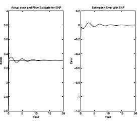
FIGURE 12.5
Extended-Kalman-Filter Performance with Unknown Initial Condition and ℓ₂-Bounded Disturbance; Reprinted from Int. J. of Robust and Nonlinear Control, RNC1643 (published online August) © 2010, “Discrete-time mixed ${\mathcal{H}}_2$/${\mathcal{H}}_{\mathrm{\infty }}$ nonlinear filtering,” by M. D. S. Aliyu and E. K. Boukas, with permission from Wiley Blackwell.

$\begin{array}{l}\tilde{Y}=-\frac{1}{2}\left[\left({\widehat{x}}^{1/5}+{\widehat{x}}^{1/3}\right)+y^2\right]+\frac{1}{2}{\left({\widehat{x}}^{1/5}+{\widehat{x}}^{1/3}\right)}^2,\\ {\tilde{V}}^1=\frac{1}{2}\left[{\left({\widehat{x}}^{1/5}+{\widehat{x}}^{1/3}\right)}^2+y^2\right].\end{array}$

Therefore,

$\begin{array}{l}{\tilde{Y}}^1\left(\widehat{x},y_{k-1}\right)=-\frac{1}{2}{\left(y-x\right)}^2-\frac{1}{2}{y}^2,\\ \tilde{V}\left(\widehat{x},y_{k-1}\right)=\frac{1}{2}{\left(y-x\right)}^2+\frac{1}{2}\left[{\left({\widehat{x}}^{1/5}+{\widehat{x}}^{1/3}\right)}^2+y^2\right].\end{array}$

We can use the above approximate solution ${\tilde{V}}^1\left(\widehat{x},y_{k-1}\right)$ to the DHJIE to estimate the states of the system, since the gain of the filter depends only on ${\tilde{V}}_{\widehat{x}}^1\left(\widehat{x},y\right)$. Consequently, we can compute the filter gain as

$l\left(x_k,y_k\right)\approx -\frac{\left(y_k-x_k\right)}{y_k-x_k^{\frac{1}{2}}-x_k^{\frac{1}{3}}}.$

(12.90)

The result of simulation with this filter is then shown in Figure 12.4. We also compare this result with that of an extended-Kalman filter for the same system shown in Figure 12.5. It can clearly be seen that, the mixed ${\mathcal{H}}_2$/${\mathcal{H}}_{\infty }$ filter performance is superior to that of the EKF.

12.4  Notes and Bibliography

This chapter is entirely based on the authors’ contributions [18, 19, 21]. The reader is referred to these references for more details.

1  A second-order Taylor series approximation would be more accurate, but the first-order method gives a solution that is very close to the continuous-time case.