C H A P T E R 15
Compute Node Layout
The term node is a fairly generic one that has many different meanings in the IT industry. For example, network engineers call any addressable device attached to their network a node. Unix administrators commonly use the term interchangeably with host or server. Oracle DBAs often refer to a database server that is a member of an RAC cluster as a node. Oracle's documentation uses the term compute node when referring to the database server tier of the platform. This chapter is about the various ways in which you can configure your Exadata compute nodes, whether they are members of an RAC cluster (nodes), or nonclustered (database servers).
It's a common misconception that an Exadata rack must be configured as a single Oracle RAC cluster. This couldn't be further from the truth. In its simplest form, the Exadata database tier can be described as a collection of independent database servers hardwired into the same storage and the same management networks. Each of these servers can be configured to run standalone databases completely independent of the others. However, this is not commonly done for a couple of reasons—scalability and high availability. Oracle RAC has historically been used to provide node redundancy in the event of node or instance failure, but Oracle marketing has made it clear all along that the ability to scale-out has been an equally important goal. Traditionally, if we needed to increase database performance and capacity, we did so by upgrading server hardware. This method became so commonplace that the industry coined the phrase “hardware refresh” to describe it. This term can mean anything from adding CPUs, memory, or I/O bandwidth to a complete replacement of the server itself. Increasing performance and capacity in this way is referred to as scale-up. With Exadata's ability to provide extreme I/O performance to the database server, bus speed is now the limiting factor for scale-up. So what happens when you reach the limits of single-server capacity? The obvious answer is to add more servers. To continue to scale your application, you must scale-out, using Oracle RAC. Nonetheless, understanding that the database servers are not tied together in some proprietary fashion clarifies the highly configurable nature of Exadata. In Chapter 14 we discussed various strategies for configuring Exadata's storage subsystems to service specific database servers. In this chapter we'll take a look at ways the database tier may be configured to create clustered and nonclustered database environments that are well suited to meet the needs of your business.
Provisioning Considerations
Exadata is an extremely configurable platform. Determining the best configuration for your business will involve reviewing the performance and uptime demands of your applications as well as ensuring adequate separation for development, test, and production systems. Here are a few of the key considerations for determining the most suitable compute node layout to support your database environments:
CPU Resources: When determining the optimal node layout for your databases, keep in mind that Exadata handles the I/O workload very differently from traditional database platforms. On non-Exadata platforms the database server is responsible for retrieving all data blocks from storage to satisfy I/O requests from the applications. Exadata offloads a lot of this work to the storage cells. This can significantly reduce the CPU requirements of your database servers. Figuring out how much less CPU your databases will require is a difficult task because it depends, in part, on how much your database is utilizing parallel query and HCC compression, and how suitable your application SQL is to offloading. Some of the Smart Scan optimizations, such as decryption, predicate filtering, and HCC decompression, will reduce CPU requirements regardless of the type of application. We covered these topics in detail in Chapters 2–6.
Systems requiring thousands of dedicated server connections can overwhelm the resources of a single machine. Spreading these connections across multiple compute nodes reduces the burden on the system's process scheduler and allows the CPU to spend its time more effectively servicing client requests. Load balancing connections across multiple compute nodes also improves the database's capacity for handling concurrent connection requests.
Memory Resources: Systems that require thousands of dedicated server connections can also put a burden on memory resources. Each dedicated server connection requires a slice of memory, whether or not the connection is actively being used. Spreading these connections across multiple RAC nodes allows the database to handle more concurrent connections than a single compute node can manage.
I/O Performance and Capacity: Each compute node and storage cell is equipped with one 40Gbps QDR, dual-port InfiniBand card through which, in practicality, each compute node can transmit/receive a maximum of 3.2 gigabytes per second. If this is sufficient bandwidth, then the decision of moving to a multi-node RAC configuration may be more of an HA consideration. If you have I/O-hungry applications that require more throughput than one compute node can provide, then RAC may be used to provide high availability as well as additional I/O capacity.
Patching and Testing: Another key consideration in designing a stable database environment is providing a separate area where patches and new features can be tested before rolling them into production. For non-Exadata platforms, patching and upgrading generally involves O/S patches and Oracle RDBMS patches. Exadata is a highly complex database platform, consisting of several additional hardware and software layers that must be patched periodically, such as Cell Server,
CellCLI, ILOM firmware, InfiniBand switch firmware, InfiniBand network card firmware, and OFED drivers. As such, it is absolutely crucial that a test environment be isolated from critical systems to be used for testing patches.
![]() Kevin Says: Regarding I/O Performance and Capacity, it is essential to understand that a producer's ability to send data is metered by the ability of the consumer to ingest the data. There is inherent flow-control in the relationship between the database grid and the storage grid in Exadata architecture. During a Smart Scan, each cell (producer) has the capacity to produce an outbound flow of data via iDB at roughly 3.2 GBps with the X2 models. But the data has to go somewhere. Scaling from this single-cell number is limited to the aggregate ingest bandwidth of the database grid (the consumers), which is 25.6 GBps for a full rack configuration. To put it another way, the X2 models can stream data unimpeded from hard disk to the database grid at full advertised scan rate (25GBps). However, when scanning both flash and hard disk assets concurrently, the full rack scan rate increases to approximately 70 GBps. Where does the excess go? It's clear to see that only about 35% of that 70 GBps can flow into the database grid. The necessary 65% payload reduction is the responsibility of Smart Scan filtration and projection. If the queries are not selective enough to reduce the payload, the result is throttled scan throughput. That leads to a related topic: effective scan rates and data flow.
Kevin Says: Regarding I/O Performance and Capacity, it is essential to understand that a producer's ability to send data is metered by the ability of the consumer to ingest the data. There is inherent flow-control in the relationship between the database grid and the storage grid in Exadata architecture. During a Smart Scan, each cell (producer) has the capacity to produce an outbound flow of data via iDB at roughly 3.2 GBps with the X2 models. But the data has to go somewhere. Scaling from this single-cell number is limited to the aggregate ingest bandwidth of the database grid (the consumers), which is 25.6 GBps for a full rack configuration. To put it another way, the X2 models can stream data unimpeded from hard disk to the database grid at full advertised scan rate (25GBps). However, when scanning both flash and hard disk assets concurrently, the full rack scan rate increases to approximately 70 GBps. Where does the excess go? It's clear to see that only about 35% of that 70 GBps can flow into the database grid. The necessary 65% payload reduction is the responsibility of Smart Scan filtration and projection. If the queries are not selective enough to reduce the payload, the result is throttled scan throughput. That leads to a related topic: effective scan rates and data flow.
For EHCC tables, the effective scan rate is equal to the physical scan rate multiplied by the compression ratio. For instance, consider an EHCC table with a compression ratio of 10:1 that fits within the capacity of a full rack Exadata Smart Flash Cache (roughly 5TB). Smart Scan will scan this table at roughly 70 GBps, but the effective scan rate is about 700 GBps. While nobody would argue that 700GBps is a phenomenal scan rate with current technology, the important question must still be asked: How selective are your queries? Considering the aggregate ingest bandwidth of a full rack X2 model, it's clear that the 700GBps effective scan rate has to be filtered down by over 96% (700GB × 25.6GB). If the filtration is not aggressive enough, the scan rate tails off because the consumer throttles the producer. Herein lies a conundrum—the selectivity of your queries must complement the compression factor of your EHCC data. The problem, however, is that query selectivity is a constant, and yet something must give. That something is physical I/O. Consider, for example, a query accessing tables with a combined footprint of 5TB so as to fit within the Exadata Smart Flash capacity of a full rack. Let's say further that this query cites very few columns and is so selective that Smart Scan is able to whittle the payload down by 95%. That would be very effective filtration and, as such, scanning flash and hard disk at a full rack rate of 70 GBps would render an iDB payload of about 3.5 GBps—a rate that doesn't even saturate two database hosts' iDB ingest bandwidth. At 70 GBps the hypothetical query completes in about 70 seconds. Can EHCC reduce the query time? For the sake of example, let's say the data in the hypothetical 5 TB table compresses tenfold with EHCC (down to roughly 500 GB). At a Smart Scan rate of 70 GBps, the query should complete in about 7 seconds, however, the data and query are the same, so the payload reduction remains constant at 95%. EHCC data is decompressed in the storage grid (after filtration and projection), so for a given query the same data flows over iDB whether noncompressed or compressed with EHCC. With payload reduction being constant, can our hypothetical query improve in a manner commensurate with the compression ratio (for example, 1/10th the time)? No, because filtering away 95%, from the effective scan rate of 700 GBps, renders an iDB demand of 35 GBps—about 37% more than the aggregate ingest bandwidth of the database grid. The scan rate is therefore throttled. The query should indeed run faster than noncompressed, but as we can see there is more to it than simple math. The hypothetical query cannot complete in 1/10th the time. In such a case the physical scan rate for the full rack would be throttled back to roughly 45 GBps, and so the query would complete in approximately 11 seconds—1/6th the time as in the noncompressed case. This example does not take into consideration any other factor that may cause consumers to throttle producers, such as join processing and sorting. It considers only the aggregate iDB ingest bandwidth in the database grid. Other factors, such as database grid CPU-saturation (due to heavy join and sort processing) can further throttle the flow of data over iDB. There is a direct correlation between the selectivity of a query, the host processor utilization level, and the performance improvement delivered by EHCC. I often have to remind people that the concept of compression as a performance feature is quite new, and often misrepresented.
Non-RAC Configuration
Compute nodes may be configured in a number of ways. If your application does not need the high availability or scale-out features of Oracle RAC, then Exadata provides an excellent platform for delivering high performance for standalone database servers. You can manage I/O service levels between independent databases by configuring the IORM. See Chapter 7 for more information about IORM. In a non-RAC configuration each compute node will have its own, non-clustered, ASM instance that provides storage for all databases on that server. Even though your database servers may be independent of one another they can still share Exadata storage (cell disks). This allows each database to make use of the full I/O bandwidth of the Exadata storage subsystem. Note that in this configuration Clusterware is not installed at all. Just like any other standalone database server, multiple databases coexist quite nicely within the same disk groups. For example, let's say you have three databases on your server, called SALES, HR, and PAYROLL. All three databases can share the same disk groups for storage. To do this, all three databases would set their instance parameters as follows:
db_create_file_dest='DATA1_DG'

db_recovery_file_dest='RECO1_DG'
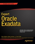
In Figure 15-1 we see all eight compute nodes in an Exadata full rack configuration running standalone databases. For example, DB1, Node 1, uses the DATA1_DG and RECO1_DG disk groups, which are serviced by the local (nonclustered) ASM instance. Each ASM instance has its own set of ASM disk groups, which consist of grid disks from all storage cells. At the storage cell, these independent ASM instances cannot share grid disks. Each ASM instance will have its own, private set of grid disks.
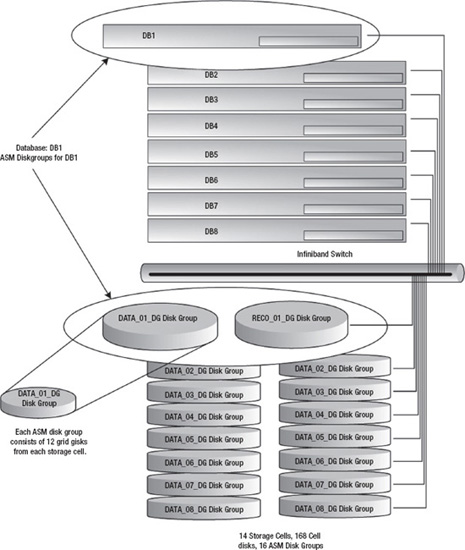
Figure 15-1. Example of a non-RAC Exadata configuration
Recall from Chapter 14 that grid disks are actually slices of cell disks. These grid disks are in turn used to create ASM disk groups. For example, each of the following commands creates twelve 200G grid disks on storage cell 1 (one per cell disk). These grid disks are then used to create the DATA1…DATA8, and RECO1…RECO8 disk groups. If all fourteen storage cells of an Exadata full rack configuration are used, it will yield 33.6 terabytes of storage (assuming 2 TB, high-capacity drives) for each disk group, ((14 storage cells × 12 grid disks per cell) × 200G).
CellCLI> CREATE GRIDDISK ALL HARDDISK PREFIX=DATA1_DG, size=200G

...

CellCLI> CREATE GRIDDISK ALL HARDDISK PREFIX=DATA8_DG, size=200G


CellCLI> CREATE GRIDDISK ALL HARDDISK PREFIX=RECO1_DG, size=200G

...

CellCLI> CREATE GRIDDISK ALL HARDDISK PREFIX=RECO8_DG, size=200G
Table 15-1 is a summary of a storage layout that supports eight standalone databases, each having a 33.6TB DATA disk group and a 33.6TB RECO disk group.
By default all ASM instances will have access to all grid disks. The following SQL query run from one of the ASM instances illustrates this. Notice how grid disks from all storage cells are flagged as candidates, that is, available for use.
SYS:+ASM1> select substr(path,16,length(path)) griddisk,

                  failgroup, header_status

             from v$asm_disk

            where substr(path,16,length(path)) like '%DATA%_DG_00%'

               or substr(path,16,length(path)) like '%RECO%_DG_00%'

            order by failgroup, substr(path,16,length(path));


GRIDDISK             FAILGROUP  HEADER_STATUS

-------------------- ---------- -------------

DATA1_CD_00_cell01   CELL01     CANDIDATE

DATA2_CD_00_cell01   CELL01     CANDIDATE

DATA3_CD_00_cell01   CELL01     CANDIDATE

DATA4_CD_00_cell01   CELL01     CANDIDATE

DATA5_CD_00_cell01   CELL01     CANDIDATE

DATA6_CD_00_cell01   CELL01     CANDIDATE

DATA7_CD_00_cell01   CELL01     CANDIDATE

DATA8_CD_00_cell01   CELL01     CANDIDATE

...

DATA1_CD_00_cell02   CELL02     CANDIDATE

DATA2_CD_00_cell02   CELL02     CANDIDATE

DATA3_CD_00_cell02   CELL02     CANDIDATE

...

DATA7_CD_00_cell03   CELL03     CANDIDATE

DATA8_CD_00_cell03   CELL03     CANDIDATE

...

RECO1_CD_00_cell01   CELL01     CANDIDATE

RECO2_CD_00_cell01   CELL01     CANDIDATE

RECO3_CD_00_cell01   CELL01     CANDIDATE

RECO4_CD_00_cell01   CELL01     CANDIDATE

RECO5_CD_00_cell01   CELL01     CANDIDATE

RECO6_CD_00_cell01   CELL01     CANDIDATE

RECO7_CD_00_cell01   CELL01     CANDIDATE

RECO8_CD_00_cell01   CELL01     CANDIDATE

...

RECO1_CD_00_cell02   CELL02     CANDIDATE

RECO2_CD_00_cell02   CELL02     CANDIDATE

RECO3_CD_00_cell02   CELL02     CANDIDATE

...

RECO7_CD_00_cell03   CELL03     CANDIDATE

RECO8_CD_00_cell03   CELL03     CANDIDATE
With this many grid disks, (2,688 in this case) visible to all ASM instances, it's easy to see how they can be accidentally misallocated to the wrong ASM disk groups. To protect yourself from mistakes like that, you might want to consider using cell security to restrict the access of each ASM instance so that it only “sees” its own set of grid disks. For detailed steps on how to implement cell security, refer to Chapter 14.
RAC Clusters
Now that we've discussed how each compute node and storage cell can be configured in a fully independent fashion, let's take a look at how they can be clustered together to provide high availability and horizontal scalability using RAC clusters. But before we do that, we'll take a brief detour and establish what high availability and scalability are.
High availability (HA) is a fairly well understood concept, but it often gets confused with fault tolerance. In a truly fault-tolerant system, every component is redundant. If one component fails, another component takes over without any interruption to service. High availability also involves component redundancy, but failures may cause a brief interruption to service while the system reconfigures to use the redundant component. Work in progress during the interruption must be resubmitted or continued on the redundant component. The time it takes to detect a failure, reconfigure, and resume work varies greatly in HA systems. For example, active/passive Unix clusters have been used extensively to provide graceful failover in the event of a server crash. Now, you might chuckle to yourself when you see the words “graceful failover” and “crash” used in the same sentence (unless you work in the airline industry), so let me explain. Graceful failover in the context of active/passive clusters means that when a system failure occurs, or a critical component fails, the resources that make up the application, database, and infrastructure are shut down on the primary system and brought back online on the redundant system automatically with as little downtime as possible. The alternative, and somewhat less graceful, type of failover would involve a phone call to your support staff at 3:30 in the morning. In active/passive clusters, the database and possibly other applications only run on one node at a time. Failover using in this configuration can take several minutes to complete depending on what resources and applications must be migrated. Oracle RAC uses an active/active cluster architecture. Failover on an RAC system commonly takes less than a minute to complete. True fault tolerance is generally very difficult and much more expensive to implement than high availability. The type of system and impact (or cost) of a failure usually dictates which is more appropriate. Critical systems on an airliner, space station, or a life support system easily justify a fault-tolerant architecture. By contrast, a web application servicing the company's retail store front usually cannot justify the cost and complexity of a fully fault-tolerant architecture. Exadata is a high-availability architecture providing fully redundant hardware components. When Oracle RAC is used, this redundancy and fast failover is extended to the database tier.
When CPU, memory, or I/O resource limits for a single server are reached, additional servers must be added to increase capacity. The term “scalability” is often used synonymously with performance. That is, increasing capacity equals increasing performance. But the correlation between capacity and performance is not a direct one. Take, for example, a single-threaded, CPU intensive program that takes 15 minutes to complete on a two-CPU server. Assuming the server isn't CPU-bound, installing two more CPUs is not going to make the process run any faster. If it can only run on one CPU at a time, it will only execute as fast as one CPU can process it. Performance will only improve if adding more CPUs allows a process to have more uninterrupted time on the processor. Neither will it run any faster if we run it on a four-node cluster. As the old saying goes, nine pregnant women cannot make a baby in one month. However, scaling out to four servers could mean that we can run four copies of our program concurrently, and get roughly four times the amount of work done in the same 15 minutes. To sum it up, scaling out adds capacity to your system. Whether or not it improves performance depends on how scalable your application is, and how heavily loaded your current system is. Keep in mind that Oracle RAC scales extremely well for well written applications. Conversely, poorly written applications tend to scale poorly.
Exadata can be configured as multiple RAC clusters to provide isolation between environments. This allows the clusters to be managed, patched, and administered independently. At the database tier this is done in the same way you would cluster any ordinary set of servers using Oracle Clusterware. To configure storage cells to service specific compute nodes, the cellip.ora file on each node lists the storage cells it will use. For example, the following cellip.ora file lists seven of the fourteen storage cells by their network address:
[enkdb01:oracle:EXDB1] /home/oracle

> cat /etc/oracle/cell/network-config/cellip.ora

cell="192.168.12.9"

cell="192.168.12.10"

cell="192.168.12.11"

cell="192.168.12.12"

cell="192.168.12.13"

cell="192.168.12.14"

cell="192.168.12.15"
When ASM starts up, it searches the storage cells on each of these IP addresses for grid disks it can use for configuring ASM disk groups. Alternatively, Cell Security can be used to lock down access so that only certain storage cells are available for compute nodes to use. The cellip.ora file and cell security are covered in detail in Chapter 14.
To illustrate what a multi-RAC Exadata configuration might look like, let's consider an Exadata V2 full rack configuration partitioned into three Oracle RAC clusters. A full rack gives us eight compute nodes and fourteen storage cells to work with. Consider an Exadata full rack configured as follows:
- One Production RAC cluster with four compute nodes and seven storage cells
- One Test RAC cluster with two compute nodes and three storage cells
- One Development RAC cluster with two compute nodes and four storage cells
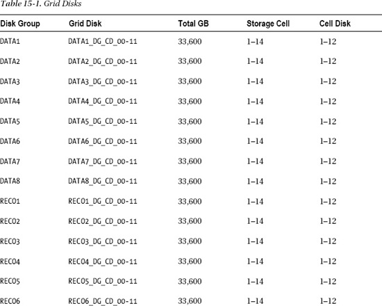
Table 15-2 shows the resource allocation of these RAC clusters, each with its own storage grid. As you read this table, keep in mind that hardware is a moving target. These figures are from an Exadata V2. In this example we used the high-capacity, 2 TB SATA disk drives.
These RAC environments can be patched and upgraded completely independently of one another. The only hardware resources they share are the InfiniBand switch and the KVM switch. If you are considering a multi-RAC configuration like this, keep in mind that patches to the InfiniBand switch will affect all storage cells and compute nodes. This is also true of the KVM switch, which is not needed to run the clusters, ASM instances, or databases; so if an issue takes your KVM switch offline for a few days, it won't impact system performance or availability. Figure 15-2 illustrates what this cluster configuration would look like.
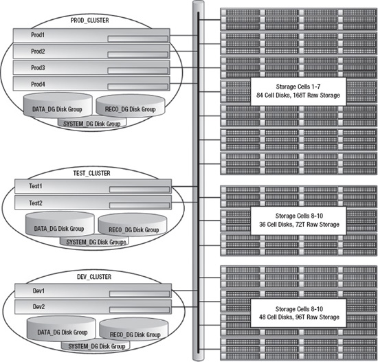
Figure 15-2. An Exadata full rack configured for three RAC clusters
Typical Exadata Configuration
The two configuration strategies we've discussed so far are fairly extreme examples. The “non-RAC Database” configuration illustrated how Exadata can be configured without Clusterware, to create a “shared nothing” consolidation platform. The second example, “RAC Clusters,” showed how Clusterware can be used to create multiple, isolated RAC clusters. Neither of these configurations is typically found in the real world, but they illustrate the configuration capabilities of Exadata. Now let's take a look at a configuration we commonly see in the field. Figure 15-3 shows a typical system with two Exadata half racks. It consists of a production cluster (PROD_CLUSTER) hosting a two-node production database and a two-node UAT database. The production and UAT databases share the same ASM disk groups (made up of all grid disks across all storage cells). I/O resources are regulated and prioritized using Exadata I/O Resource Manager (IORM), discussed in Chapter 7. The production database uses Active Data Guard to maintain a physical standby for disaster recovery and reporting purposes. The UAT database is not considered business-critical, so it is not protected with Data Guard. On the standby cluster (STBY_CLUSTER), the Stby database uses four of the seven storage cells for its ASM storage. On the development cluster (DEV_CLUSTER), the Dev database uses the remaining three cells for its ASM storage. The development cluster is used for ongoing product development and provides a test bed for installing Exadata patches, database upgrades, and new features.
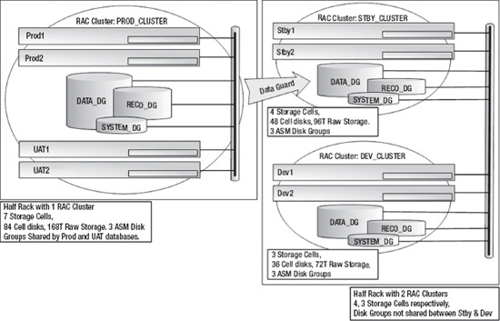
Figure 15-3. A typical configuration
Exadata Clusters
Exadata's ability to scale out doesn't end when the rack is full. When one Exadata rack doesn't quite get the job done for you, additional racks may be added to the cluster, creating a large-scale database grid. Up to eight racks may be cabled together to create a massive database grid, consisting of 64 database servers and 2,688 terabytes of storage. Actually, Exadata will scale beyond eight racks, but additional InfiniBand switches must be purchased to do it. Exadata links cabinets together using what Oracle calls a spine switch. The spine switch is included with all half rack and full rack configurations. Quarter rack configurations do not have a spine switch and cannot be linked with other Exadata racks. In a full rack configuration, the ports of a leaf switch are used as follows:
- Eight links to the database servers
- Fourteen links to the storage cells
- Seven links to the redundant leaf switch
- One link to the spine switch
- Six ports open
Figure 15-4 shows an Exadata full rack configuration that is not linked to any other Exadata rack. It's interesting that Oracle chose to connect the two leaf switches together using the seven spare cables. Perhaps it's because these cables are preconfigured in the factory, and patching them into the leaf switches simply keeps them out of the way and makes it easier to reconfigure later. The leaf switches certainly do not need to be linked together. The link between the leaf switches and the spine switch doesn't serve any purpose in this configuration, either. It is only used if two or more Exadata racks are linked together.
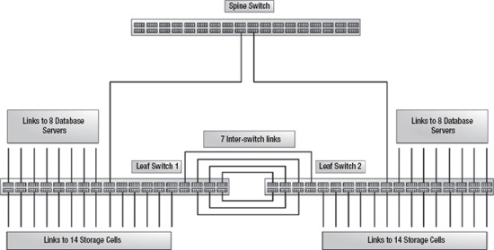
Figure 15-4. An Exadata full rack InfiniBand network
The spine switch is just like the other two InfiniBand switches that service the cluster and storage network. The diagram may lead you to wonder why Oracle would make every component in the rack redundant except the spine switch. The answer is that redundancy is provided by connecting each leaf switch to every spine switch in the configuration (from two to eight spine switches).
To network two Exadata racks together, the seven inter-switch cables, seen in Figure 15-4, are redistributed so that four of them link the leaf switch with its internal spine switch, and four of them link the leaf switch to the spine switch in the adjacent rack. Figure 15-5 shows the network configuration for two Exadata racks networked together. When eight Exadata racks are linked together, the seven inter-switch cables seen in Figure 15-4 are redistributed so that each leaf-to-spine-switch link uses one cable (eight cables per leaf switch). When you're linking from three to seven Exadata racks together, the seven inter-switch cables are redistributed as evenly as possible across all leaf-to-spine-switch links. Leaf switches are not linked to other leaf switches, and spine switches are not linked to other spine switches. No changes are ever needed for the leaf switch links to the compute nodes and storage cells.
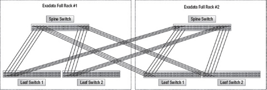
Figure 15-5. A switch configuration for two Exadata racks, with one database grid
Summary
Exadata is a highly complex, highly configurable database platform. In Chapter 14, we talked about all the various ways disk drives and storage cells can be provisioned separately, or in concert, to deliver well balanced, high-performance I/O to your Oracle databases. In this chapter we turned our attention to provisioning capabilities and strategies at the database tier. Exadata is rarely used to host standalone database servers. In most cases it is far better suited for Oracle RAC clusters. Understanding that every compute node and storage cell is a fully independent component is important, so we spent a considerable amount of time showing how to provision eight standalone compute nodes on an Exadata full rack configuration. From there we moved on to an Oracle RAC provisioning strategy that provided separation between three computing environments. And finally, we touched on how Exadata racks may be networked together to build massive database grids. Understanding the concepts explored in Chapter 14 and 15 of this book will help you make the right choices when the time comes to architect a provisioning strategy for your Exadata database environment.