C H A P T E R 13
Migrating to Exadata
So the day is finally here. Your Exadata Database Machine is installed, configured, tuned, tweaked and ready to go. By now you’ve probably invested many, many hours learning about Exadata, proving its value to the company, and planning how you will make the most of this powerful database platform. No doubt it has been a long road to travel but you aren’t there quite yet. Now the real work begins—migration.
This was a much more difficult chapter to write than we expected. We can’t count all the migrations we’ve been through over the years. But when we considered all the various versions of Oracle, the migration tools available, and how they have changed from one version to the next, it became clear that we needed to narrow the scope somewhat. So to keep this interesting and save a few trees we’ll be focusing on version 11.2 Enterprise Edition for a majority of this chapter. Along the way we’ll point out ways to make the most of the features available in previous versions of the Oracle database.
There are many methods, tools, and techniques for migrating your database from legacy hardware to Exadata, but generally speaking they fall into two broad categories: physical migration and logical migration. While there are several factors that determine which method is best, the decision making process is usually dominated by one factor, the available down time to complete the move. The good news is that there are several strategies to help you get there. Each method comes with its own pro’s and con’s. In this chapter we’re going to dig into each of these methods. We’ll talk about reasons you might use one over the other, the relative advantages and disadvantages, and what common pitfalls you should watch out for.
![]() Note: Migrating your applications to Oracle Exadata from non-Oracle platforms is out of the scope of this book, so it won’t be covered here.
Note: Migrating your applications to Oracle Exadata from non-Oracle platforms is out of the scope of this book, so it won’t be covered here.
![]() Kevin Says: During Technical Review I approached this chapter with skepticism. In my thinking, the idea of an entire chapter dedicated to migrating a database to the Exadata Database Machine seemed like a waste of space. Allow me to explain.
Kevin Says: During Technical Review I approached this chapter with skepticism. In my thinking, the idea of an entire chapter dedicated to migrating a database to the Exadata Database Machine seemed like a waste of space. Allow me to explain.
I routinely remind people that unless Exadata Hybrid Columnar Compression (EHCC) is being used, there is no difference between data segments stored in Exadata Storage Server cells and those in conventional storage. The Oracle Database software deployed in the Exadata Database Machine is Oracle Database 11g—with a very small amount of code that knows how to compress data into EHCC form and otherwise interface with Exadata via iDB. I conducted my first review pass of this chapter with the mindset of an imaginary customer who, for whatever reason, finds no need for EHCC. With that mindset I expected this chapter to be nothing more than an overview of database migration concepts, an occasional reference to Oracle product documentation, and perhaps, a paragraph or two of special handling considerations for EHCC. However, after my first reading of the chapter I felt compelled to add this note to the reader. Even if you know everything there is to know about database migration, in the context of Oracle database, I encourage you to read this chapter. Having said that, I still wish to reinforce the principle that there is no difference between a database stored in Exadata Storage Server cells and one stored in conventional storage—unless HCC is involved. To end up with an Oracle database stored in Exadata Storage Server cells, you have to flow the data through the database grid using the same tools used for any other migration to Oracle. However, I believe that the principles conveyed in this chapter will be quite helpful in any migration scenario to Oracle. I consider that a bonus!
Migration Strategies
Once you have a good understanding what Exadata is, and how it works, you are ready to start thinking about how you are going to get your database moved. Migration strategies fall into two general categories, logical migration and physical migration. Logical migration involves extracting the data from one database and loading it into another. Physical migration refers to lifting the database, block by block, from one database server and moving it to another. The data access characteristics of your database are a key consideration when deciding which migration method is best. This is primarily because of the way the data is accessed on Exadata. OLTP databases tend to use single block reads and update data across all tables, whereas Data Warehouse (DW) databases are typically optimized for full table scans and only update current data. Exadata uses Flash Cache on the storage cells to optimize single block reads and improve the overall performance for OLTP databases. For DW databases Exadata uses Smart Scan technology to optimize full table scans. The details of these two optimization methods are covered in Chapters 2 and 5. Logical migration allows you the opportunity to make changes to your database to optimize it for the Exadata platform. Such changes might include resizing extents, implementing or redesigning your current partitioning schemes, and compressing tables using HCC. These are all very important storage considerations for large tables and especially so for DW databases. Because OLTP applications tend to update data throughout the database, HCC compression is not a good fit and would actually degrade performance. And while large extents (4MB and 8MB+) are beneficial for DW databases, they are less advantageous for OLTP databases, which use mostly index-based access and “random” single-block reads. Physical migration, by its very nature, allows no changes to be made to the storage parameters for tables and indexes in the database, while logical migration allows much more flexibility in redefining storage, compression, partitioning and more.
Logical Migration
Regardless of the technology used, logical migration consists of extracting objects from the source database and reloading them into a target database. Even though logical migration strategies tend to be more complicated than physical strategies, they are usually preferable because of the following advantages:
Staged Migration :Tables and partitions that are no longer taking updates can be moved outside of the migration window, reducing the volume to be moved during the final cut over.
Selective Migration: Often times the source database has obsolete user accounts and database objects that are no longer needed. With the logical method these objects may be simply omitted from the migration. The old database may be kept around for awhile in case you later decide you need something that didn’t get migrated.
Platform Differences: Data is converted to target database block size automatically. Big-endian to little-endian conversion is handled automatically.
Exadata hybrid columnar compression (HCC) can be configured before data is moved. That is the tables may be defined with HCC in the Exadata database so that data is compressed as it is loaded into the new database.
Extent Sizing: Target tables, partitions, and indexes may be pre-created with optimal extent sizes (multiples of 4MB) before the data is moved.
Allows Merging of Databases: This is particularly important when Exadata is used as a consolidation platform. If your Exadata is model V2 or X2-2, memory on the database servers may be a somewhat limiting factor. V2 database servers are configured with 72G of RAM each, while X2-2 comes with 96G RAM per server. This is a lot of memory when dealing with 10 or fewer moderate to large sized databases. But it is becoming fairly common to see 15 or more databases on a server. For example, one of us worked on a project where Exadata was used to host PeopleSoft HR and Financials databases. The implementer requested 15 databases for this effort. Add to this the 10 databases in their plan for other applications and SGA memory became a real concern. The solution of course is to merge these separate databases together allowing them to share memory more efficiently. This may or may not be a difficult task depending on how contained the databases are at the schema level.
If using the “create table as select” method or “insert into as select” method (CTAS or IAS) over a database link, then the data may also be sorted as it is loaded into the target database to improve index efficiency, optimize for Exadata Storage Indexes and achieve better compression ratios.
There are basically two approaches for logical migration. One involves extracting data from the source database and loading it into the target database. We’ll call this the “Extract and Load” method. Tools commonly used in this approach are Data Pump, Export/Import, and CTAS (or IAS) through a database link. The other method is to replicate the source database during normal business operations. When the time comes to switch to the new database, replication is cancelled and client applications are redirected to the new database. We’ll refer to this as the “Replication-Based” method. Tools commonly used in the Replication-Based method are Oracle Streams, Oracle Data Guard (Logical Standby), and Oracle Golden Gate. It is also possible to use a combination of physical and logical migration, such as copying (mostly) read only tablespaces over well ahead of the final cut-over and applying changes to them via some replication method like Streams.
Extract and Load
Generally speaking, the Extract and Load method requires the most downtime of all the migration strategies. This is because once the extract begins, and for the duration of the migration, all DML activity must be brought to a stop. Data warehouse environments are the exception to the rule, because data is typically organized in an “age-in/age-out” fashion. Since data is typically partitioned by date range, static data is separated from data that is still undergoing change. This “read only” data may be migrated ahead of time, outside the final migration window; perhaps even during business hours. The biggest advantage of the Extract and Load strategy is its simplicity. Most DBAs have used Data Pump or CTAS for one reason or another, so the tool set is familiar. Another big advantage is the control it gives you. One of the great new features Exadata brings to the table is Hybrid Columnar Compression (HCC). Since you have complete control over how the data is loaded into the target database, it is a relatively simple task to employ HCC to compress tables as they are loaded in. Extract and Load also allows you to implement partitioning or change partitioning strategies. Loading data using CTAS allows you to sort data as it is loaded, which improves the efficiency of Exadata’s storage indexes. One could argue that all these things could be done post migration, and that is true. But why move the data twice when it can be incorporated into the migration process itself? In some situations it may not even be possible to fit the data onto the platform without applying compression. In the next few sections we will cover several approaches for performing Extract and Load migrations.
![]() Kevin Says: The point about ordered loading of data is a very important topic. It is true that this may not always be an option, but the benefit can go even further than the improved storage index efficiency already mentioned. Ordered loading can increase the compression ratio of Exadata Hybrid Columnar Compression as well. In spite of the sophisticated load-time compression techniques employed by the HCC feature, the fundamentals can never be forgotten. In the case of compression, like-values always compress more deeply. It is worth considering whether this approach fits into the workflow and opportunity window for data loading.
Kevin Says: The point about ordered loading of data is a very important topic. It is true that this may not always be an option, but the benefit can go even further than the improved storage index efficiency already mentioned. Ordered loading can increase the compression ratio of Exadata Hybrid Columnar Compression as well. In spite of the sophisticated load-time compression techniques employed by the HCC feature, the fundamentals can never be forgotten. In the case of compression, like-values always compress more deeply. It is worth considering whether this approach fits into the workflow and opportunity window for data loading.
Data Pump
Data Pump is an excellent tool for moving large quantities of data between databases. Data Pump consists of two programs, expdp and impdp. The expdp command is used to extract database objects out of the source database. It can be used to dump the contents of an entire database or, more selectively, by schema or by table. Like its predecessor Export (exp), Data Pump extracts data and saves it into a portable data file. This file can then be copied to Exadata and loaded into the target database using the impdp command. Data Pump made its first appearance in Oracle 10g, so if your database is version 9i or earlier, you will need to use the old Export/Import (exp/imp) instead. Export and Import have been around since Oracle 7, and although they are getting a little long in the tooth they are still very effective tools for migrating data and objects from one database to another. And, even though Oracle has been talking about dropping exp and imp for years now, they are still part of the base 11.2 install. First we’ll talk about Data Pump and how it can be used to migrate to Exadata. After that we can take a quick look at ways to migrate older databases using Export and Import. Keep in mind that new features and parameters are added to Data Pump with each major release. Check the Oracle documentation for capabilities and features specific to your database version.
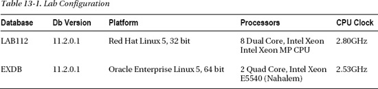
From time to time in this chapter we’ll make reference to tests and timings we saw in our lab. Table 13-1 shows some of the relevant characteristics of the servers and databases we used for these tests. The LAB112 database is the source database and EXDB is the target (Exadata) database. It is an Exadata V2 quarter rack configuration.
Here is a breakdown of the segments in my test database.
SEGMENT_TYPE               MBYTES

-------------------- ------------

CLUSTER                        63

INDEX                      13,137

INDEX PARTITION               236

LOBINDEX                       48

LOBSEGMENT                    290

TABLE                      20,662

TABLE PARTITION             1,768

TYPE2 UNDO                    142
Now, let’s take a look at some of the Data Pump parameters you’ll want to know about. Here are some of the key parameters that are useful for migrating databases.
COMPRESSION: Data Pump compression is a relatively new feature. In 10g you had the ability to compress metadata, but in 11g this capability was extended to table data as well. Valid options areALL,DATA_ONLY,METADATA_ONLYandNONE. Using theCOMPRESSION=ALLoption Data Pump reduced the size of our export from 13.4G to 2.5G, a compression ratio of over 5 times. That’s a pretty significant savings in storage. When we ran the test with compression turned on, we fully expected it to slow down the export, but instead it actually reduced our export time from 39 minutes to just over 9 minutes. This won’t always be the case, of course. On our test system the export was clearly I/O-bound. But it does point out that compression can significantly reduce the storage requirements for exporting your database without necessarily slowing down the process. Unfortunately, the ability to compress table data on the fly was not introduced until release 11gR1. If your database is 10g and you need to compress your dumpfiles before transferring them to Exadata, you will need to do that using external tools like gzip, zip, or compress. Note that the use of the dataCOMPRESSIONoption in Data Pump requires Oracle Advanced Compression licenses.
FLASHBACK_TIME,FLASHBACK_SCN: Believe it or not, by default Data Pump does not guarantee the read consistency of your export. To export a read-consistent image of your database you must use either theFLASHBACK_SCNor theFLASHBACK_TIMEparameter. If you useFLASHBACK_TIME, Data Pump looks up the nearest System Change Number (SCN) corresponding to the time you specified and exports all data as of that SCN.FLASHBACK_TIMEcan be passed in to Data Pump as follows:FLASHBACK_TIME="to_timestamp('05-SEP-2010 21:00:00','DD-MON-YYYY HH24:MI:SS')"If you choose to use
FLASHBACK_SCN, you can get the current SCN of your database by running the following query:SQL> select current_scn from v$database;
FULL,SCHEMAS,TABLES: These options are mutually exclusive and specify whether the export will be for the full database, a selection of schemas, or a selection of individual tables. Note that certain schemas, like SYS, MDSYS, CTXSYS, and DBSNMP, are never exported when doing a full database export.
PARALLEL: ThePARALLELparameter instructs Data Pump to split the work up into multiple parts and run them concurrently.PARALLELcan vastly improve the performance of the export process.
NETWORK_LINK: This parameter specifies a database link in the target database to be used for the export. It allows you to export a database from a remote server, pull the data directly through the network via database link (in the target database), and land the files on an Exadata file system. We see this as more of a convenience than anything else, as it saves you the extra step of transporting the dumpfiles manually at the end of the export. It is used by Grid Control to automate the migration process using the “Import From Database” process. Using this method for manual migration doesn’t make much sense— if you are going to copy the data over a database link anyway, why not load it to target tables directly, using CTAS or direct-path insert, instead of dumping it to disk and reloading back later on?
Now let’s turn our attention to the import process. Schema-level import is usually preferable when migrating databases. It allows you to break the process up into smaller, more manageable parts. This is not always the case, and there are times when a full database import is the better choice. Most of the tasks we will talk about here apply to both schema-level and full database imports, As we go along, we’ll note any exceptions you will need to be aware of. If you choose not to do a full database import, be aware that system objects including roles, public synonyms, profiles, public database links, system privileges, and others will not be imported. You will need to extract the DDL for these objects using the SQLFILE parameter and a FULL=Y import. You can then execute the DDL into the target database to create them. Let’s take a look at some of the parameters useful for migrating databases.
REMAP_SCHEMA: As the name implies, this parameter tells Data Pump to change the ownership of objects from one schema to another during the course of the import. This is particularly useful for resolving schema conflicts when merging multiple databases into one Exadata database.
REMAP_DATAFILE: Datafiles can be renamed dynamically during the import process using this parameter. This allows ASM to automatically organize and name the datafiles according to Oracle Managed Files (OMF) rules.
REMAP_TABLESPACE: This option changes the tablespace name reference for segments from one tablespace to another. It is useful when you want to physically relocate tables from one tablespace to another during the import.
SCHEMAS: List of schemas to import.
SQLFILE: Instead of importing anything into the database, Object definitions (DDL) are written to an SQL script. This can be quite useful for pre-building objects if you want to make changes to their physical structure, such as partitioning or using HCC compression.
TABLE_EXISTS_ACTION: The action to take if the imported object already exists. Valid keywords areAPPEND,REPLACE,[SKIP], andTRUNCATE.
TABLES: A list of tables to import. For example,TABLES=KSO.SKEW, RJOHNSON.TEST
TRANSFORM: This parameter allows you to make changes to segment attributes in object-creation DDL statements, like storage attributes. This provides a convenient way to optimize extent sizes for tables when they are created in Exadata.
Before you begin importing schemas into your Exadata database, be aware that Data Pump only creates tablespaces automatically when a full database import is done. So if you are importing at the schema or table level you will need to create your tablespaces manually. To do this, generate the DDL for tablespaces using the parameters FULL=yes and SQLFILE={your_sql_script}. This produces a script with the DDL for all objects in the dumpfile, (including datafiles). One thing you may notice about the CREATE TABLESPACE DDL is that the datafile file names are fully qualified. This isn’t at all what we want, because it circumvents OMF and creates hard-coded file names that cannot be managed by the database. The REMAP_DATAFILE parameter allows you to rename your datafiles to reflect the ASM disk groups in your Exadata database. The syntax looks something like this:
REMAP_DATAFILE='/u02/oradata/LAB112/example01.dbf':'+DATA'One final note before we move on to Export/Import. Character set translation between the source and target databases is done automatically with Data Pump. Make sure the character set of the source database is a subset of the target database, or something may be lost in translation. For example, it’s okay if your source database is US7ASCII (7 bit) and the target database is WE8ISO8859P1 (8 bit). But migrating between different 8-bit character sets or going from 8 bit to 7 bit may cause special characters to be dropped.
Export and Import
If the database you are migrating to Exadata is a release prior to version 10g, Data Pump won’t be an option. Instead you will need to work with its predecessors, Export (exp) and Import (imp). Export/Import features haven’t changed much since Oracle 9.2, but if you are migrating from a previous release, you will notice that some features may be missing. Hopefully you aren’t still supporting 8i databases, or God forbid 7.x, but not to worry. Even though some options like FLASHBACK_SCN and PARALLEL are not options in these older releases, there are ways to work around these missing features.
PARALLEL is strictly a Data Pump feature but you can still parallelize database exports by running concurrent schema exports. This is a much less convenient way of “parallelizing” your export process. If you have to parallelize your export process in this way you will have to do the work of figuring out which schemas, grouped together, are fairly equal in size to minimize the time it takes for all of them to complete.
COMPRESSION is another feature missing from Export. This has never been much of an issue for DBAs supporting Unix/Linux platforms. These systems provide the ability to redirect the output from Export through the compress or gzip commands by means of a named pipe, something like this (the $ sign is the shell prompt, of course):
$ mkfifo exp.dmp


$ ls -l exp.dmp

prw-rw-r-- 1 rjohnson dba 0 Oct  2 15:17 exp.dmp


$ cat exp.dmp | gzip -c > my_compressed_export.dmp.gz &


$ exp system file=exp.dmp owner=rjohnson consistent=y compress=n statistics=none log=my_compressed_export.log


$ ls -l my_compressed_export.*

-rw-rw-r-- 1 rjohnson dba 3134148165 Oct  2 22:32 my_compressed_export.dmp.gz

-rw-rw-r-- 1 rjohnson dba       1432 Oct  2 22:32 my_compressed_export.log
The REMAP_TABLESPACE parameter is not available in Export/Import. To work around this you will have to generate a SQL file using the INDEXFILE parameter which produces a SQL script like Data Pump’s SQLFILE parameter. You can then modify tablespace references and pre-create segments in the new tablespace as needed. Using the IGNORE parameter will allow Import to simply perform an insert into the tables you manually created ahead of time. The REMAP_SCHEMA parameter takes on a slightly different form in Import. To change the name of a schema during import, use the FROMUSER and TOUSER parameters.
There is one limitation with Export/Import that cannot be escaped. Import does not support Exadata Hybrid Columnar Compression (HCC). Our tests show that when importing data using Import, the best table compression you can expect to get is about what you would get with tables compressed for OLTP (also known in 11g as “Advanced Compression”). It doesn’t matter if a table is configured for any one of the four HCC compression modes available on Exadata, (Query Low/High and Archive Low/High). This is because HCC compression can only occur if the data is direct-path inserted, using syntax like insert /*+ APPEND */, for example. According the Exadata User’s Guide, “Conventional inserts and updates are supported,” but “result in a less compressed format, and reduced compression ratio.” This “reduced compression ratio” is actually the same as the OLTP compression provided by the Advanced Compression option, which HCC falls back to for normal inserts. By the way, Import will not complain or issue any warnings to this effect. It will simply import the data at a much lower compression rate, silently eating up far more storage than you planned or expected. There is nothing you can do about it other than rebuild the affected tables after the import is complete. The important thing to understand is that you cannot exploit Exadata’s HCC compression using Export/Import.
The Export/Import approach also does not support Transparent Data Encryption (TDE). If your database uses TDE you will need to use Data Pump to migrate this data. If you are importing at the schema level, system objects like roles, public synonyms, profiles, public database links, system privileges, and others will not be imported. System objects like these can be extracted by doing a full database import and with the INDEXFILE parameter to extract the DDL to create these objects. This step is where the most mistakes are made. It is a tedious process and careful attention must be given so that nothing falls through the cracks. Fortunately, there are third-party tools that do a very good job of comparing two databases and showing you where you’ve missed something. Most of these tools, like TOAD and DB Change Manager from Embarcadero, also provide a feature to synchronize the object definitions across to the new database.
If you are still thinking about using Export/Import, note that as the data loading with Import doesn’t use direct-path load inserts, it will have much higher CPU usage overhead due to undo and redo generation and buffer cache management. You would also have to use a proper BUFFER parameter for array inserts (you’ll want to insert thousands of rows at a time) and use COMMIT=Y (which will commit after every buffer insert) so you wouldn’t fill up the undo segments with one huge insert transaction.
When to Use Data Pump or Export/Import
Data Pump and Export/Import are volume-sensitive operations. That is, the time it takes to move your database will be directly tied to its size and the bandwidth of your network. For OLTP applications this is downtime. As such, it is better suited for smaller OLTP databases. It is also well suited for migrating large DW databases, where read-only data is separated from read-write data. Take a look at the downtime requirements of your application and run a few tests to determine whether Data Pump is a good fit. Another benefit of Data Pump and Export/Import is that they allow you to copy over all the objects in your application schemas easily, relieving you from manually having to copy over PL/SQL packages, views, sequence definitions, and so on. It is not unusual to use Export/Import for migrating small tables and all other schema objects, while the largest tables are migrated using a different method.
What to Watch Out for when Using Data Pump or Export/Import
Character-set differences between the source and target databases are supported, but if you are converting character sets make sure the character set of the source database is a subset of the target. If you are importing at the schema level, check to be sure you are not leaving behind any system objects, like roles and public synonyms, or database links. Remember that HCC is only supported in Data Pump. Be sure you use the consistency parameters of Export or Data Pump to ensure that your data is exported in a read-consistent manner. Don’t forget to take into account the load you are putting on the network.
Data Pump and Export/Import methods also require you to have some temporary disk space (both in the source and target server) for holding the dumpfiles. Note that using Data Pump’s table data compression option requires you to have Oracle Advanced Compression licenses both for the source and target database (only the metadata_only compression option is included in the Enterprise Edition license).
Copying Data over a Database Link
When extracting and copying very large amounts of data—many terabytes—between databases, database links may be your best option. Unlike the DataPump option, with database links you will read your data once (from the source), transfer it immediately over the network, and write it once (into the target database). With Data Pump, Oracle would have to read the data from source, then write it to a dumpfile, and then you’ll transfer the file with some file-transfer tool (or do the network copy operation using NFS), read the dumpfile in the target database, and then write it into the target database tables. In addition to all the extra disk I/O done for writing and reading the dumpfiles, you would need extra disk space for holding these dumpfiles during the migration. Now you might say “Hold on, DataPump does have the NETWORK_LINK option and the ability to transfer data directly over database links.” Yes that’s true, but unfortunately when using impdp with database links, Data Pump performs conventional INSERT AS SELECTs, not direct path inserts. And this means that the inserts will be much slower, generate lots of redo and undo, and possibly run out of undo space. And more importantly, conventional path IAS does not compress data with HCC compression (but resorts to regular OLTP compression instead if HCC is enabled for the table). So this makes the DataPump file-less import over database links virtually useless for loading lots of data into Exadata fast. You would have to use your own direct path IAS statements with APPEND hints to get the benefits of direct path loads and maximum performance out of file-less transfer over database links.
![]() Kevin Says: Add to this list of possible dumpfile transfer techniques the capability known as Injecting Files with Database File System (DBFS). The DBFS client (
Kevin Says: Add to this list of possible dumpfile transfer techniques the capability known as Injecting Files with Database File System (DBFS). The DBFS client (dbfs_client) has been ported to all Linux and Unix platforms and can be used to copy files into the Exadata Database Machine even if the DBFS file system is not mounted on the hosts of the Exadata Database Machine nor on the sending system. It is a mount-free approach. Oracle Documentation provides clear examples of how to use the built-in copy command that dbfs_client supports. The data flows from the dbfs_client executable over SQL*Net and is inserted directly into SecureFile LOBs. The transfer is much more efficient than the NFS protocol and is secure. Most Exadata Database Machine deployments maintain DBFS file systems, so there is less of a need for local disk capacity used as a staging area.
There are some cases where moving your data through database links may not perform as well as the DataPump approach. If you have a slow network link between the source and target (migrations between remote data centers, perhaps) then you may benefit more from compressing the dumpfiles, while database links over Oracle Net won’t do as aggressive compression as, for example, gzip can do. Oracle Net (SQL*Net) does simple compression by de-duplicating common column values within an array of rows when sent over SQL*Net. This is why the number of bytes transferred over SQL*Net may show a smaller value than the total size of raw data.
Transferring the data of a single table over a database link is very easy. In the target (Exadata) database you’ll need to create a database link pointing to the source database, then just issue either a CTAS or INSERT SELECT command over the database link:
CREATE DATABASE LINK sourcedb

    CONNECT TO source_user

    IDENTIFIED BY source_password

    USING 'tns_alias';


CREATE TABLE fact AS SELECT * FROM fact@sourcedb;
This example will create the table structure and copy the data, but it won’t create any other objects such as indexes, triggers or constraints for the table. These objects must be manually created later, either by running the DDL scripts or by doing a metadata-only import of the schema objects.
![]() Note: When creating the database link, you can specify the database link’s TNS connect string directly, with a USING clause, like this:
Note: When creating the database link, you can specify the database link’s TNS connect string directly, with a USING clause, like this:
CREATE DATABASE LINK ... USING '(DESCRIPTION = (ADDRESS = (PROTOCOL = TCP)(HO/ST =
localhost)(PORT = 1521)) (CONNECT_DATA = (SERVER = DEDICATED) (SERVICE_NAME = ORA10G)))'
That way, you don’t have to set up tnsnames.ora entries in the database server.
Another option is to use INSERT SELECT for loading data into an existing table structure. We want to bypass the buffer cache, and the undo-generation-and-redo-logging mechanism for this bulk data load, so we can use the APPEND hint to make this a direct path load insert:
INSERT /*+ APPEND */ INTO fact SELECT * FROM fact@sourcedb;


COMMIT;
We’re assuming here that the database is in NOARCHIVELOG mode during the migration, so we haven’t set any logging attributes for the table being loaded. In NOARCHIVELOG mode all bulk operations (such as INSERT APPEND, index REBUILD and ALTER TABLE MOVE) are automatically NOLOGGING.
If your database must be in ARCHIVELOG mode during such data loading, but you still want to perform the loading of some tables without logging, then you can just temporarily turn off logging for those tables for the duration of the load:
ALTER TABLE fact NOLOGGING;


INSERT /*+ APPEND */ INTO fact SELECT * FROM fact@sourcedb;


ALTER TABLE fact LOGGING;
Of course if your database or tablespace containing this table is marked FORCE LOGGING, then logging will still occur, despite any table-level NOLOGGING attributes.
Achieving High-Throughput CTAS or IAS over a Database Link
While the previous examples are simple, they may not give you the expected throughput, especially when the source database server isn’t in the same LAN as the target. The database links and the underlying TCP protocol must be tuned for high throughput data transfer. The data transfer speed is limited obviously by your networking equipment throughput and is also dependent on the network round-trip time (RTT) between the source and target database.
When moving tens of terabytes of data in a short time, you obviously need a lot of network throughput capacity. You must have such capacity from end to end, from your source database to the target Exadata cluster. This means that your source server must be able to send data as fast as your Exadata cluster has to receive it, and any networking equipment (switches, routers) in between must also be able to handle that, in addition to all other traffic that has to flow through them. Dealing with corporate network topology and network hardware configuration is a very wide topic and out of the scope of this book, but we’ll touch the subject of the network hardware built in to Exadata database servers here.
In addition to the InfiniBand ports, Exadata clusters also have built-in Ethernet ports. Table 13-2 lists all the Ethernet and InfiniBand ports.
Note that this table shows the number of network ports per database server. So, while Exadata V2 does not have any 10GbE ports, it still has 4 × 1GbE ports per database server. With 8 database servers in a full rack, this would add up to 32 × 1 GbE ports, giving you a maximum theoretical throughput of 32 gigabits per second when using only Ethernet ports. With various overheads, 3 gigabytes per second of transfer speed would theoretically still be achievable if you manage to put all of the network ports equally into use and there are no other bottlenecks. This would mean that you have to either bond the network interfaces or route the data transfer of different datasets via different network interfaces. Different dblinks’ connections can be routed via different IPs or DataPump dumpfiles transferred via different routes.
This already sounds complicated, that’s why companies migrating to Exadata often used the high-throughput bonded InfiniBand links for migrating large datasets with low downtime. Unfortunately, the existing database networking infrastructure in most companies does not include InfiniBand (in old big iron servers). The standard usually is a number of switched and bonded 1 GbE Ethernet ports or 10 GbE ports in some cases. That’s why, for Exadata V1/V2 migrations, you would have had to either install an InfiniBand card into your source server or use a switch capable of both handling the source Ethernet traffic and flowing it on to the target Exadata InfiniBand network.
Luckily the new Exadata X2-2 and X2-8 releases both have 10 GbE ports included in them, so you don’t need to go through the hassle of getting your old servers InfiniBand-enabled anymore and can resort to 10 GbE connections (if your old servers or network switches have 10GbE Ethernet cards in place). Probably by the time this book comes out, nobody plans large-scale migrations to Exadata V1 and V2 anymore.
![]() Note: Remember that if you do not have huge data transfer requirements within a very low downtime window, then the issues described here may not be problems for you at all. You would want to pick the easiest and simplest data transfer method that gets the job done within the required time window. It’s important to know the amount of data to be transferred in advance and test the actual transfer speeds in advance to see whether you would fit into the planned downtime. If your dblink transfer or dumpfile copy operation is too slow, then you can use free tools like iPerf (
Note: Remember that if you do not have huge data transfer requirements within a very low downtime window, then the issues described here may not be problems for you at all. You would want to pick the easiest and simplest data transfer method that gets the job done within the required time window. It’s important to know the amount of data to be transferred in advance and test the actual transfer speeds in advance to see whether you would fit into the planned downtime. If your dblink transfer or dumpfile copy operation is too slow, then you can use free tools like iPerf (http://iperf.sourceforge.net) to test out your network throughput between source and target servers. If the dblinks or datapump dumpfile transfer is significantly worse than iPerf’s results, there must be a configuration bottleneck somewhere.
This leads us to software configuration topics for high network throughput for database migrations. This chapter does not aim to be a network tuning reference, but we would like to explain some challenges we’ve seen. Getting the Oracle database links throughput right involves changing multiple settings and requires manual parallelization. Hopefully this section will help you avoid reinventing the wheel when dealing with huge datasets and low downtime requirements.
In addition to the need for sufficient throughput capacity at the network hardware level, there are three major software configuration settings that affect Oracle’s data transfer speed:
- Fetch array size (
arraysize) - TCP send and receive buffer sizes
- Oracle Net Session Data Unit (SDU) size
With regular application connections, the fetch array size has to be set to a high value, ranging from hundreds to thousands, if you are transferring lots of rows. Otherwise, if Oracle sends too few rows out at a time, most of the transfer time may end up being spent waiting for SQL*Net packet ping-pong between the client and server.
However, with database links, Oracle is smart enough to automatically set the fetch array size to the maximum—it transfers 32767 rows at a time. So, we don’t need to tune it ourselves.
Tuning TCP Buffer Sizes
The TCP send and receive buffer sizes are configured at the operating-system level, so every O/S has different settings for it. In order to achieve higher throughput, the TCP buffer sizes have to be increased in both ends of the connection. We’ll cover a Linux and Solaris example here; read your O/S networking documentation if you need to do this on other platforms. We often use the Pittsburgh Supercomputing Center’s “Enabling High Performance Data Transfers” page for reference (http://www.psc.edu/networking/projects/tcptune/). First, you’ll need to determine the maximum buffer size TCP (per connection) in your system.
On the Exadata servers, just keep the settings for TCP buffer sizes as they were set during standard Exadata install. On Exadata the TCP stack has already been changed from generic Linux defaults. Do not configure Exadata servers settings based on generic database documentation (such as the “Oracle Database Quick Installation Guide for Linux”).
However, on the source system, which is about to send large amounts of data, the default TCP buffer sizes may become a bottleneck. You should add these lines to /etc/sysctl.conf if they’re not there already:
net.core.rmem_default = 262144

net.core.rmem_max = 1048576

net.core.wmem_default = 262144

net.core.wmem_max = 4194304
Then issue a sysctl –p command to apply these values into the running kernel.
The maximum read and write buffer sizes per TCP connection will be set to 1MB and 4MB respectively, but the default starting value for buffers is 256kB for each. Linux kernels 2.4.27 (and higher) and 2.6.17 (and higher) can automatically tune the actual buffer sizes from default values up to allowed maximums during runtime. If these parameters are not set, Linux kernel (2.6.18) defaults to 128kB buffer sizes, which may become a bottleneck when transferring large amounts of data. The write buffer has been configured bigger as the source data would be sending (writing) the large amounts of data, the amount of data received will be much smaller.
The optimal buffer sizes are dependent on your network roundtrip time (RTT) and the network link maximum throughput (or desired throughput, whichever is lower). The optimal buffer size value can be calculated using the Bandwidth*Delay product (BDP) formula, also explained in the “Enabling High Performance Data Transfers” document mentioned earlier in this section. Note that changing the kernel parameters shown earlier means a global change within the server, and if your database server has a lot of processes running, the memory usage may rise thanks to the increased buffer sizes. So you might not want to increase these parameters until the actual migration happens.
Here’s an example from another O/S type. On Solaris 8 and newer versions, the default send and receive buffer size is 48KB. This would result in even poorer throughput compared to Linux’s default 128KB. On Solaris you can check the max buffer size and max TCP congestion window with the following commands:
$ ndd /dev/tcp tcp_max_buf

1048576

$ ndd /dev/tcp tcp_cwnd_max

1048576
This output shows that the maximum (send or receive) buffer size in the Solaris O/S is 1MB. This can be changed with the ndd –set command, but you’ll need root privileges for that:
# ndd - set/dev/tcp tcp_max_buf 4194304

# ndd - set/dev/tcp tcp_cwnd_max 4194304
This, however just sets the maximum TCP buffer sizes (and the TCP congestion window) per connection, but not the default buffer sizes, which a new connection would actually get. The default buffer sizes can be read this way:
$ ndd /dev/tcp tcp_xmit_hiwat

49152

$ ndd /dev/tcp tcp_recv_hiwat

49152
Both the default send buffer (xmit means transmit) and receive buffer sizes are 48KB. To change these defaults to 4MB each, we would run these commands:
# ndd -set /dev/tcp tcp_recv_hiwat 4194304

# ndd -set /dev/tcp tcp_xmit_hiwat 4194304
Note that these settings are not persistent, they will be lost after a reboot. If you want to persist these settings, you should add a startup script into rc3.d (or some rc.local equivalent), which would re-run the previous commands. Another option would be to put these values to /etc/system, but starting from Solaris 10 the use of the global /etc/system settings is not encouraged. Yet another approach would be to put the values into a Solaris Service Management Framework (SMF) manifest file, but that is out of the scope of this book.
If the source server is still going to be actively in use (in production) during the data transfer, then think twice before increasing the default buffer sizes globally. While you could potentially make the bulk data transfer much faster for everybody with larger buffer sizes, your server memory usage would also grow (TCP buffers live in kernel memory) and you could run into memory shortage issues.
This is where a more sophisticated way for changing buffer sizes becomes very useful. Solaris allows you to set the default send and receive buffer sizes at route level. So, assuming that the target server is in a different subnet from most other production servers, you can configure the buffer sizes for a specific route only.
Let’s check the current routes first:
# netstat -rn

Routing Table: IPv4

  Destination           Gateway           Flags  Ref     Use     Interface

-------------------- -------------------- ----- ----- ---------- ---------

default              192.168.77.2         UG        1          0 e1000g0

default              172.16.191.1         UG        1          1

172.16.0.0           172.16.191.51        U         1          2 e1000g1

192.168.77.0         192.168.77.128       U         1          3 e1000g0

224.0.0.0            192.168.77.128       U         1          0 e1000g0

127.0.0.1            127.0.0.1            UH        1         82 lo0
Let’s assume that that the target Exadata server uses subnet 192.168.77.0, and one of the servers has IP 192.168.77.123. You can use the route get command in the Solaris machine to see if there are any existing route-specific settings:
# route get 192.168.77.123

   route to: 192.168.77.123

destination: 192.168.77.0

       mask: 255.255.255.0

  interface: e1000g0

      flags: <UP,DONE>

 recvpipe  sendpipe  ssthresh    rtt,ms rttvar,ms  hopcount      mtu     expire

       0         0         0         0         0         0      1500         0
The recvpipe and sendpipe values are zero; they use whatever are the O/S system-wide defaults. Let’s change the route settings now and check the settings with route get again:
# route change -net 192.168.77.0 -recvpipe 4194304 -sendpipe 4194304

change net 192.168.77.0

# route get 192.168.77.123

   route to: 192.168.77.123

destination: 192.168.77.0

       mask: 255.255.255.0

  interface: e1000g0

      flags: <UP,DONE>

 recvpipe  sendpipe  ssthresh    rtt,ms rttvar,ms  hopcount      mtu     expire

 4194304   4194304         0         0         0         0      1500         0
Now all connections between the source server and that subnet would request both send and receive socket buffer size 4 MB, but connections using other routes would continue using default values.
Note that this route change setting isn’t persistent across reboots, so you would need to get the sysadmin to add this command in a Solaris (or SMF service) startup file.
Before you change any of these socket buffer setting at the O/S level, there’s some good news if your source database is Oracle 10g or newer. Starting from Oracle 10g, it is possible to make Oracle request a custom buffer size itself (up to the tcp_max_buf limit) when a new process is started. You can do this by changing the listener.ora on the server side (source database) and tnsnames.ora (or the raw TNS connect string in database link definition) in the target database side. The target database acts as the client in the database link connection pointing from target to source. This is well documented in the Optimizing Performance section of the Oracle Database Net Services Administrator’s Guide, section “Configuring I/O Buffer Size.”
Additionally, you can reduce the number of syscalls Oracle uses for sending network data, by increasing the Oracle Net Session Data Unit (SDU) size. This requires either a change in listener.ora or setting the default SDU size in server-side sqlnet.ora. Read the Oracle documentation for more details. Here is the simplest way to enable higher SDU and network buffer in Oracle versions 10g and newer.
Add the following line to the source database’s sqlnet.ora:
DEFAULT_SDU_SIZE=32767Make sure the source database’s listener.ora contains statements like the following example:
LISTENER =

  (DESCRIPTION_LIST =

    (DESCRIPTION =

      (ADDRESS = (PROTOCOL = IPC)(KEY = EXTPROC1521))

      (ADDRESS =

        (PROTOCOL = TCP)

        (HO/ST = solaris01)

        (PORT = 1521)

        (SEND_BUF_SIZE=4194304)

        (RECV_BUF_SIZE=1048576)

      )

    )

  )
The target Exadata server’s tnsnames.ora would then look like this example:
SOL102 =

  (DESCRIPTION =

    (SDU=32767)

    (ADDRESS =

      (PROTOCOL = TCP)

      (HO/ST = solaris01)

      (PORT = 1521)

      (SEND_BUF_SIZE=1048576)

      (RECV_BUF_SIZE=4194304)

    )

    (CONNECT_DATA =

      (SERVER = DEDICATED)
      (SERVICE_NAME = SOL102)

    )

  )
With these settings, when the database link connection is initiated in the target (Exadata) database, the tnsnames.ora connection string additions will make the target Oracle database request a larger TCP buffer size for its connection. Thanks to the SDU setting in the target database’s tnsnames.ora and the source database’s sqlnet.ora, the target database will negotiate the maximum SDU size possible—32767 bytes.
![]() Note: If you have done SQL*Net performance tuning in old Oracle versions, you may remember another SQL*Net parameter:
Note: If you have done SQL*Net performance tuning in old Oracle versions, you may remember another SQL*Net parameter: TDU (Transmission Data Unit size). This parameter is obsolete and is ignored starting with Oracle Net8 (Oracle 8.0).
It is possible to ask for different sizes for send and receive buffers. This is because during the data transfer the bulk of data will move from source to target direction. Only some acknowledgement and “fetch more” packets are sent in the other direction. That’s why we’ve configured the send buffer larger in the source database (listener.ora) as the source will do mostly sending. On the target side (tnsnames.ora), we’ve configured the receive buffer larger as the target database will do mostly receiving. Note that these buffer sizes are still limited by the O/S-level maximum buffer size settings (net.core.rmem_max and net.core.wmem_max parameters in /etc/sysctl.conf in Linux and tcp_max_buf kernel setting in Solaris).
Parallelizing Data Load
If you choose the extract-load approach for your migration, there’s one more bottleneck to overcome in case you plan to use Exadata Hybrid Columnar Compression (EHCC). You probably want to use EHCC to save the storage space and also get better data scanning performance (compressed data means fewer bytes to read from disk). Note that faster scanning may not make your queries significantly faster if most of your query execution time is spent in operations other than data access, like sorting, grouping, joining and any expensive functions called either in the SELECT list or filter conditions. However, EHCC compression requires many more CPU cycles than the classic block-level de-duplication, as the final compression in EHCC is performed with heavy algorithms (LZO, ZLib or BZip, depending on the compression level). Also, while decompression can happen either in the storage cell or database layer, the compression of data can happen only in the database layer. So, if you load lots of data into a EHCC-compressed table using a single session, you will be bottlenecked by the single CPU you’re using. Therefore you’ll need to parallelize the data load to take advantage of all the database layer’s CPUs to get the data load done faster.
Sounds simple—we’ll just add a PARALLEL flag to the target table or a PARALLEL hint into the query, and we should be all set, right? Unfortunately things are more complex than that. There are a couple of issues to solve; one of them is easy, but the other one requires some effort.
Issue 1—Making Sure the Data Load Is Performed in Parallel
The problem here is that while parallel Query and DDL are enabled by default for any session, the parallel DML is not. Therefore, parallel CTAS statements will run in parallel from end to end, but the loading part of parallel IAS statements will be done in serial! The query part (SELECT) will be performed in parallel, as the slaves pass the data to the single Query Coordinator and the QC is the single process, which is doing the data loading (including the CPU-intensive compression).
This problem is simple to fix, though; you’ll just need to enable parallel DML in your session. Let’s check the parallel execution flags in our session first:
SQL> SELECT pq_status, pdml_status, pddl_status, pdml_enabled

  2> FROM v$session WHERE sid = SYS_CONTEXT('userenv','sid'),


PQ_STATUS PDML_STATUS PDDL_STATUS PDML_ENABLED

--------- ----------- ----------- ---------------

ENABLED   DISABLED    ENABLED     NO
The parallel DML is disabled in the current session. The PDML_ENABLED column is there for backward compatibility. Let’s enable PDML:
SQL> ALTER SESSION ENABLE PARALLEL DML;


Session altered.


SQL> SELECT pq_status, pdml_status, pddl_status, pdml_enabled

  2> FROM v$session WHERE sid = SYS_CONTEXT('userenv','sid'),


PQ_STATUS PDML_STATUS PDDL_STATUS PDML_ENABLED

--------- ----------- ----------- ---------------

ENABLED   ENABLED     ENABLED     YES
After enabling parallel DML, the INSERT AS SELECTs are able to use parallel slaves for the loading part of the IAS statements.
Here’s one important thing to watch out for, regarding parallel inserts. In the next example we have started a new session (thus the PDML is disabled in it), and we’re issuing a parallel insert statement. We have added a “statement-level” PARALLEL hint into both insert and query blocks, and the explained execution plan output (the DBMS_XPLAN package) shows us that parallelism is used. However, this execution plan would be very slow loading into a compressed table, as the parallelism is enabled only for the query (SELECT) part, not the data loading part!
Pay attention to where the actual data loading happens—in the LOAD AS SELECT operator in the execution plan tree. This LOAD AS SELECT, however, resides above the PX COORDINATOR row source (this is the row source that can pull rows and other information from slaves into QC). Also, in line 3 you see the P->S operator, which means that any rows passed up the execution plan tree from line 3 are received by a serial process (QC).
SQL> INSERT /*+ APPEND PARALLEL(16) */ INTO t2 SELECT /*+ PARALLEL(16) */ * FROM t1


---------------------------------------------------------------------------------------

| Id  | Operation                     | Name     | Rows  |    TQ  |IN-OUT| PQ Distrib |

---------------------------------------------------------------------------------------

|   0 | INSERT STATEMENT              |          |  8000K|        |      |            |

|   1 |  LOAD AS SELECT               | T2       |       |        |      |            |

|   2 |   PX COORDINATOR              |          |       |        |      |            |

|   3 |    PX SEND QC (RANDOM)        | :TQ10000 |  8000K|  Q1,00 | P->S | QC (RAND)  |

|   4 |     PX BLOCK ITERATOR         |          |  8000K|  Q1,00 | PCWC |            |

|   5 |      TABLE ACCESS STORAGE FULL| T1       |  8000K|  Q1,00 | PCWP |            |

---------------------------------------------------------------------------------------


Note

-----

   - Degree of Parallelism is 16 because of hint


16 rows selected.
The message “Degree of Parallelism is 16 because of hint” means that a request for running some part of the query with parallel degree 16 was understood by Oracle and this degree was used in CBO calculations, when optimizing the execution plan. However, as explained above, this doesn’t mean that this parallelism was used throughout the whole execution plan. It’s important to check whether the actual data loading work (LOAD AS SELECT) is done by the single QC or by PX slaves.
Let’s see what happens when we enable parallel DML:
SQL> ALTER SESSION ENABLE PARALLEL DML;


Session altered.


SQL> INSERT /*+ APPEND PARALLEL(16) */ INTO t2 SELECT /*+ PARALLEL(16) */ * FROM t1


---------------------------------------------------------------------------------------

| Id  | Operation                     | Name     | Rows  |    TQ  |IN-OUT| PQ Distrib |

---------------------------------------------------------------------------------------

|   0 | INSERT STATEMENT              |          |  8000K|        |      |            |

|   1 |  PX COORDINATOR               |          |       |        |      |            |

|   2 |   PX SEND QC (RANDOM)         | :TQ10000 |  8000K|  Q1,00 | P->S | QC (RAND)  |

|   3 |    LOAD AS SELECT             | T2       |       |  Q1,00 | PCWP |            |

|   4 |     PX BLOCK ITERATOR         |          |  8000K|  Q1,00 | PCWC |            |

|   5 |      TABLE ACCESS STORAGE FULL| T1       |  8000K|  Q1,00 | PCWP |            |

---------------------------------------------------------------------------------------


Note

-----

   - Degree of Parallelism is 16 because of hint
Now, compare this plan to the previous one. They are different. In this case the LOAD AS SELECT operator has moved down the execution plan tree, it’s not a parent of PX COORDINATOR anymore. How you can read this simple execution plan is that the TABLE ACCESS STORAGE FULL sends rows to PX BLOCK ITERATOR (which is the row-source who actually calls the TABLE ACCESS and passes it the next range of data blocks to read). PX BLOCK ITERATOR then sends rows back to LOAD AS SELECT, which then immediately loads the rows to the inserted table, without passing them to QC at all. All the SELECT and LOAD work is done within the same slave, there’s no interprocess communication needed. How do we know that? It is because the IN-OUT column says PCWP (Parallel operation, Combined With Parent) for both operations, and the TQ value for both of the operations is the same (Q1,00). This indicates that parallel execution slaves do perform all these steps, under the same Table Queue node, without passing the data around between slave sets.
The proper execution plan when reading data from a database link looks like this:
SQL> INSERT /*+ APPEND PARALLEL(16) */ INTO tmp

  2> SELECT /*+ PARALLEL(16) */ * FROM dba_source@srcdb


-----------------------------------------------------------------------------------

| Id  | Operation               | Name       | Rows  | TQ/Ins |IN-OUT| PQ Distrib |

-----------------------------------------------------------------------------------

|   0 | INSERT STATEMENT        |            |   211K|        |      |            |

|   1 |  PX COORDINATOR         |            |       |        |      |            |

|   2 |   PX SEND QC (RANDOM)   | :TQ10001   |   211K|  Q1,01 | P->S | QC (RAND)  |

|   3 |    LOAD AS SELECT       | TMP        |       |  Q1,01 | PCWP |            |

|   4 |     PX RECEIVE          |            |   211K|  Q1,01 | PCWP |            |

|   5 |      PX SEND ROUND-ROBIN| :TQ10000   |   211K|        | S->P | RND-ROBIN  |

|   6 |       REMOTE            | DBA_SOURCE |   211K|  SRCDB | R->S |            |

-----------------------------------------------------------------------------------


Remote SQL Information (identified by operation id):

----------------------------------------------------


   6 - SELECT /*+ OPAQUE_TRANSFORM SHARED (16) SHARED (16) */

           "OWNER","NAME","TYPE","LINE","TEXT"

       FROM "DBA_SOURCE" "DBA_SOURCE" (accessing 'SRCDB' )


Note

-----

Degree of Parallelism is 16 because of hint
In this example, because we enabled parallel DML at the session level, the data loading is done in parallel; the LOAD AS SELECT is a parallel operation (the IN-OUT column shows PCWP) executed within PX slaves and not the QC.
Note that DBMS_XPLAN shows the SQL statement for sending to the remote server over the database link (in the Remote SQL Information section above). Instead of sending PARALLEL hints to the remote server, an undocumented SHARED hint is sent, which is an alias of the PARALLEL hint.
This was the easier issue to fix. If your data volumes are really big, then there is another problem to solve with database links, and it’s explained below.
Issue 2—Achieving Fully Parallel Network Data Transfer
Another issue with database links and parallel execution is that even if you manage to run parallel execution on both ends of the link, it is the query coordinators that actually open the database link and do the network transfer. The PX slaves don’t somehow magically open their own database link connections to the other database, all traffic flows through the single query coordinator of a query. So you can run your CTAS/IAS statement with hundreds of PX slaves—but you’ll still have only a single database link connection doing network transfer. While you can optimize the network throughput by increasing the TCP buffer and SDU sizes, there’s still a limit of how much data the QC process (on a single CPU) is able to ingest.
Figure 13-1 illustrates how the data flows through a single query coordinators despite all the parallel execution.
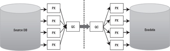
Figure 13-1. Data flow is single-threaded through query coordinators.
In addition to the single QC database link bottleneck, sending data (messages) between the QC and PX slaves takes some extra CPU time. This is where fine-tuning the parallel_execution_message_size parameter has helped a little in the past, but starting from Oracle 11.2 its value defaults to 16KB anyway, so there probably won’t be any significant benefit in adjusting this further. And if you are doing parallel data loads across multiple nodes in a RAC instance, there will still be a single QC per query with a single network connection. So, if QC runs in node 1 and the parallel slaves in node 2, the QC will have to send the data it fetches across the dblink to the PX slaves over the RAC interconnect as PX messages.
So if you choose to use database links with parallel slaves, you should run multiple separate queries in different instances and force the PX slaves to be in the same instance as the QC, using the following command:
SQL> ALTER SESSION SET parallel_force_local = TRUE;


Session altered.
That way you will avoid at least the RAC inter-instance traffic and remote messaging CPU overhead, but the QC to PX slave intra-instance messaging (row distribution) overhead still remains here.
Now, despite all these optimizations and migrating different large tables using parallel queries in different instances, you may still find that a single database link (and query coordinator) does not provide enough throughput to migrate the largest fact tables of your database within your downtime. As stated earlier, the database links approach is best used for the few huge tables in your database, and all the rest can be exported/imported with Data Pump. Perhaps you only have couple of huge fact tables, but if you have eight RAC instances in the full rack Exadata cluster, how could you make all the instances transfer and load data efficiently? You would want to have at least one parallel query with its query coordinator and database link per instance and likely multiple such queries if a single QC process can’t pull and distribute data fast enough.
The obvious solution here is to take advantage of partitioning, as your large multi-terabyte tables are likely partitioned in the source database anyway. So you can copy the huge table in multiple separate parts. However there are a couple of problems associated with this approach.
The first issue is that when performing the usual direct path load insert (which is needed for Hybrid Columnar Compression and for NOLOGGING loads), your session would lock the table it inserts into exclusively for itself. Nobody else can modify nor insert into that table while there is an uncommitted direct path load transaction active against that table. Note that others can still read that table, as SELECT statements don’t take enqueue locks on tables they select from.
So, how to work around this concurrency issue? Luckily Oracle INSERT syntax allows you to specify the exact partition or subpartition where you want to insert, by its name:
INSERT /*+ APPEND */

INTO

    fact PARTITION ( Y20080101 )

SELECT

    *

FROM

    fact@sourcedb

WHERE

    order_date >= TO_DATE('20080101 ', 'YYYYMMDD ')

AND order_date  < TO_DATE('20080102', 'YYYYMMDD ')
With this syntax, the direct-path insert statement would lock only the specified partition, and other sessions could freely insert into other partitions of the same table. Oracle would still perform partition key checking, to ensure that data wouldn’t be loaded into wrong partitions. If you attempt to insert an invalid partition key value into a partition, Oracle returns the error message:
ORA-14401: inserted partition key is outside specified partition.Note that we did not use the PARTITION ( partition_name ) syntax in the SELECT part of the query. The problem here is that the query generator (unparser), which composes the SQL statement to be sent over the database link, does not support the PARTITION syntax. If you try it, you will get an error:
ORA-14100: partition extended table name cannot refer to a remote object.That’s why we are relying on the partition pruning on the source database side—we just write the filter predicates in the WHERE condition so that only the data in the partition of interest would be returned. In the example just shown, the source table is range-partitioned by order_date column; and thanks to the WHERE clause passed to the source database, the partition pruning optimization in that database will only scan through the required partition and not the whole table.
Note that we are not using the BETWEEN clause in this example, as it includes both values in the range specified in the WHERE clause, whereas Oracle Partitioning option’s “values less than” clause excludes the value specified in DDL from the partition’s value range.
It is also possible to use subpartition-scope insert syntax, to load into a single subpartition (thus locking only a single subpartition at time). This is useful when even a single partition of data is too large to be loaded fast enough via a single process/database link, allowing you to split your data into even smaller pieces:
INSERT /*+ APPEND */

INTO

    fact SUBPARTITION ( Y20080101_SP01 )

SELECT

    *

FROM

    fact@sourcedb

WHERE

    order_date >= TO_DATE('20080101 ', 'YYYYMMDD ')

AND order_date  < TO_DATE('20080102', 'YYYYMMDD ')

AND ORA_HASH(customer_id, 63, 0) + 1 = 1
In this example the source table is still range-partitioned by order_date, but it is hash partitioned to 64 subpartitions. As it’s not possible to send the SUBPARTITION clause through the database link, either, we have used the ORA_HASH function to fetch only the rows belonging to the first hash subpartition of 64 total subpartitions. The ORA_HASH SQL function uses the same kgghash() function internally, which is used for distributing rows to hash partitions and subpartitions. If we had 128 subpartitions, we would change the 63 in the SQL syntax to 127 (n – 1).
As we would need to transfer all the subpartitions, we would copy other subpartitions in parallel, depending on the server load of course, by running slight variations of the above query and changing only the target subpartition name and the ORA_HASH output to corresponding subpartition position.
INSERT /*+ APPEND */

INTO

    fact SUBPARTITION ( Y20080101_SP02 )

SELECT

    *

FROM

    fact@sourcedb

WHERE

    order_date >= TO_DATE('20080101 ', 'YYYYMMDD ')

AND order_date  < TO_DATE('20080102', 'YYYYMMDD ')

AND ORA_HASH(customer_id, 63, 0) + 1 = 2
And so you’ll need to run a total of 64 versions of this script:
... INTO fact SUBPARTITION ( Y20080101_SP03 )  ... WHERE ORA_HASH(customer_id, 63, 0) + 1 = 3

...

... INTO fact SUBPARTITION ( Y20080101_SP04 )  ... WHERE ORA_HASH(customer_id, 63, 0) + 1 = 4

...

... INTO fact SUBPARTITION ( Y20080101_SP64 )  ... WHERE ORA_HASH(customer_id, 63, 0) + 1 = 64

...
If your table’s hash subpartition numbering scheme in the subpartition name doesn’t correspond to the real subpartition position (the ORA_HASH return value), then you’ll need to query DBA_TAB_SUBPARTITIONS and find the correct subpartition_name using the SUBPARTITION_PO/SITION column.
There’s one more catch though. While the order_date predicate will be used for partition pruning in the source database, the ORA_HASH function won’t—the query execution engine just doesn’t know how to use the ORA_HASH predicate for subpartition pruning. In other words, the above query will read all 64 subpartitions of a specified range partition, then the ORA_HASH function will be applied to every row fetched and the rows with non-matching ORA_HASH result will be thrown away. So, if you have 64 sessions, each trying to read one subpartition with the above method, each of them would end up scanning through all subpartitions under this range partition, this means 64 × 64 = 4096 subpartition scans.
We have worked around this problem by creating views on the source table in the source database. We would create a view for each subpartition, using a script, of course. The view names would follow a naming convention such as V_FACT_Y2008010_SP01, and each view would contain the SUBPARTITION ( xyz ) clause in the view’s SELECT statement. Remember, these views would be created in the source database, so there won’t be an issue with database links syntax restriction. And when it’s time to migrate, the insert-into-subpartition statements executed in the target Exadata database would reference appropriate views depending on which subpartition is required. This means that some large fact tables would have thousands of views on them. The views may be in a separate schema, as long as the schema owner has read rights on the source table. Also, you probably don’t have to use this trick on all partitions of the table, as if your largest tables are time-partitioned by some order_date or similar, then you can probably transfer much of the old partitions before the downtime window, so you won’t need to use such extreme measures.
The techniques just discussed may seem quite complicated and time consuming, but if you have tens or hundreds of terabytes of raw data to extract, transfer, and compress, and all this has to happen very fast, such measures are going to be useful. We have used these techniques for migrating VLDB data warehouses up to 100TB in size (compressed with old-fashioned block compression) with raw data sets exceeding a quarter of a petabyte. However, we need to optimize our own time too, so read the next section about when it is feasible to go with database links and when it is not.
When to Use CTAS or IAS over Database Links
If you have allocated plenty of downtime, and the database to be migrated isn’t too big, and you don’t want to do major reorganization of your database schemas, then you probably don’t have to use data load over database links. A full DataPump export/import is much easier if you have the downtime and disk space available; everything can be exported and imported with a simple command.
However, when you are migrating VLDBs with low downtime windows, database links can provide one performance advantage—with database links you don’t have to dump the data to a disk file just to copy it over and reload it back in the other server. Also, you don’t need any intermediate disk space for keeping dumps when using database links. With database links you read the data from disk once (in the source database), transfer it over the wire, and write it to disk once in the target.
Transferring lots of small tables may actually be faster with the Export/Import or Data Pump method. Also, the other schema objects (views, sequences, PL/SQL, and so on) have to be somehow migrated anyway. So it’s a good idea to transfer only the large tables over database links and use Export/Import or Data Pump for migrating everything else. And by the way, Data Pump has a nice EXCLUDE: parameter you can use for excluding the large manually transferred tables from an export job.
What to Watch Out For When Copying Tables over Database Links
Copying tables during business hours can impact performance on the source database. It can also put a load on the network, sometimes even when dedicated network hardware is installed for reducing the impact of high-throughput data transfer during production time.
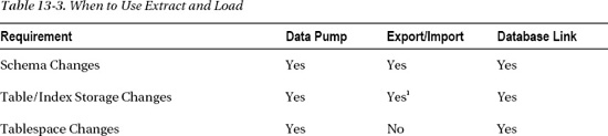
Table 13-3 shows a summary of the capabilities of each of these Extract and Load methods.

Replication-Based Migration
Generally speaking, replication-based migration is done by creating a copy of the source database and then keeping it in sync by applying changes to the copy, or “target database.” There are two very different methods for applying these changes. Physical replication ships archived redo logs to the target where it is applied to the database using its internal recovery mechanisms. This is called “Redo Apply”. We’ll talk more about how that works in the “Physical Migration” section later in this chapter. With logical replication, changes to the source database are extracted as SQL statements and executed on the target database. The technique of using SQL statements to replicate changes from source to target is called SQL Apply. Back in the 90,s when Oracle 7 and 8 were all the rage, it was common practice among DBAs to use snapshots to keep tables in a remote database in sync with master tables in the source database. These snapshots used triggers to capture changes to the master table and execute them on the target. Snapshot logs were used to queue up these changes when the target tables were unavailable so they could be executed at a later time. It was a simple form of logical replication. Of course, this was fine for a handful of tables but it became unwieldy when replicating groups of tables or entire schemas. In later releases Oracle wrapped some manageability features around this technology and branded it ”Simple Replication.” Even back in the early days of database replication there were companies that figured out how to mine database redo logs to capture DML more efficiently and less intrusively than triggers could. Today there are several products on the market that do a very good job of using this “log mining” technique to replicate databases. The advantage logical replication has over physical replication is in its flexibility. For example, logical replication allows the target to be available for read access. In some cases it also allows you to implement table compression and partitioning in the target database. In the next few sections we’ll discuss several tools that support replication-based migration.
Oracle Streams and Golden Gate
Oracle Streams is included in the base RDBMS product and was introduced as a new feature in version 9i. Golden Gate is a product recently acquired by Oracle. Both products replicate data in much the same way. A copy of the source database is created (the target) and started up. This may be done from a full database backup using Recovery Manager or by using Data Pump to instantiate SELECT schemas. Then changes in the source database are extracted, or mined, from the redo logs. The changes are then converted to equivalent DML and DDL statements and executed in the target database. Oracle calls these steps Capture, Stage, and Apply.
Regardless of which product you use, the target database remains online and available for applications to use while replication is running. New tables may be created in the target schema or in other schemas. Any restrictions on the target are limited to the tables being replicated. This is particularly useful when your migration strategy involves consolidation—taking schemas from multiple source databases and consolidating them into one database. Because of its extremely high performance and scalability, most companies use Exadata for database consolidation to at least some degree, so this is a very useful feature. If you read between the lines, you realize that this means you can migrate multiple databases concurrently.
Another capability of both Streams and Golden Gate is the ability to do data transformation. This is not something we would normally associate with database migration, but it is available should you need it. Since Streams uses SQL Apply to propagate data changes to the target, you can implement changes to the target tables to improve efficiencies. For example, you can convert conventional target tables to partitioned tables. You can also add or drop indexes and change extent sizes to optimize for Exadata. Be aware that even though replication provides this capability, it can get messy. If you are planning a lot of changes to the source tables consider implementing them before you begin replication.
Tables in the target database may be compressed using Exadata HCC. Be prepared to test performance when inserting data and using HCC compression. It is a CPU-intensive process, much more so than Basic and OLTP compression. However, the rewards are pretty significant in terms of storage savings and query performance, depending on the nature of the query of course. If conventional inserts or updates are executed on HCC-compressed tables, Oracle switches to OLTP compression (for the affected rows) and your compression ratio drops significantly. Direct path inserts can be done by implementing the insert append hint as follows:
insert /*+ append */ into my_hcc_table select ...;


insert /*+ append_values */ into my_hcc_table values ( <array of rows> );
Note that the append_values hint only works from Oracle 11gR2 onwards.
Also note that as of this writing, Golden Gate does not support reading changes of compressed tables yet. There are three bug/enhancement requests outstanding for adding extraction support for tables compressed with regular, OLTP, and HCC compression. As far as writing the data to the replication target goes, we ran some tests in our lab and found that we were able to achieve the “reduced” compression ratio by using Golden Gate’s direct load feature. It didn’t appear to support the higher levels of compression you would expect from bulk inserts. Table 13-4 shows the results of our compression tests.

As for Streams, the documentation says that direct path inserts are not supported in 10g databases. 11g does provide limited support through the Direct Path API. Once again, make sure you check the Oracle documentation to see what is supported for your database version. If in doubt run a few tests to see whether you do get the level of compression you expect. However, a big improvement in Oracle 11.2 allows Streams to capture data from tables compressed with basic table compression and OLTP compression. From Oracle 11.2.0.2 patchset onwards, Streams/XStream can also capture changes to HCC compressed tables. The Oracle Streams Concepts and Administration Guide for 11g Release 2 (11.2) explains this in more detail. This feature gives Streams a big advantage over Golden Gate if your source tables are compressed and the compressed data is updated, thus requiring some sort of change capture unless you want to copy all that data during downtime.
The list of data types Streams does not support is fairly short in version 11gR2. Here is the list from the Oracle documentation:
BFILEROWID- User-defined types (including object types,
REFs, varrays, and nested tables) XMLTypestored object relationally or as binary XML- The following Oracle-supplied types:
Anytypes, URI types, spatial types, and media types
And here is the list of unsupported data types in Golden Gate:
The following is a quick summary of the benefits common to both Oracle Streams and Golden Gate:
- Support for failover (Oracle RAC environments)
- Support for multi-tenant databases
- Support for table partitioning (target tables)
- Support for HCC compression (target tables only for Golden Gate) although you may not get the best loading compression ratio compared to CTAS or IAS
- Support for storage changes for tables and indexes (target tables)
- Ability to change indexing strategy (target tables)
- Read access to the target tables during migration
- Support for endian differences between source and target
- Support for character set differences between source and target
- Support for different database block sizes between source and target
- Support for change Capture on the target server, reducing the performance impact on the source system
- Not difficult to setup
- Database version-agnostic
- Very little downtime to switch over
Disadvantages common to both Streams and Golden Gate:
- Replicated tables must be keyed. If there is no primary key on the source table, you must provide a list of columns that provide uniqueness. If no such combination exists, the table cannot be replicated.
- Some data types are not supported for replication.
- Log mining on the source system can impact performance. Consider moving the change Capture to the target system.
- It’s more complex than other migration strategies.
Disadvantages of Streams compared to Golden Gate:
- Data mining can heavily impact performance on the source database.
- It is more complex to set up.
- DDL is supported but problematic.
- If replication breaks, fixing it can be messy. It is often easier to scrap the target and rebuild it.
- SQL Apply is more prone to falling behind the source than Golden Gate.
- Streams tends to require much more CPU resources than Golden Gate.
Advantages of Streams over Golden Gate:
- Streams is included with your database license, while Golden Gate is sold separately
- If the source database is Oracle 11.2 (or higher), Streams supports capturing changes to compressed source tables (basic and OLTP compression). If both the source and target databases are running Oracle version 11.2.0.2 or higher, then the Streams supports capturing changes to HCC compressed tables too.
- All process information is stored in the database, providing convenient remote access.
- There is integration with Grid Control.
So which should you use, Streams or Golden Gate? We’ve spoken with clients and colleagues who have used both products. In every case they are using the product for simple replication to a remote site much like you would for database migration. The feedback we get is overwhelmingly in favor of Golden Gate. These users cite Golden Gate’s ease of use, stability, and performance as the most important reasons. In addition to this, Golden Gate supports non-Oracle database sources. Streams runs inside the Oracle database and has not been ported to any other database platform. As mentioned, Streams is included in your Oracle database license. Golden Gate is not, and the cost based on the total number of cores on the source and target servers is not trivial. If you have need for data replication beyond your Exadata migration, then the investment may be well worth it. If you are faced with a one-time migration, Streams may be a better fit for cost.
When to Use Streams or Golden Gate
Streams and Golden Gate both provide a lot of flexibility with near-zero downtime. They are well suited for migrations that require changes to the target tables. This includes resizing table and index extents, implementing partitioning strategies, and compressing tables. They also allow you to change schemas, tablespaces, and disk groups, among other things.
What to Watch Out for with Streams and Golden Gate
Since Streams and Golden Gate propagate database changes by mining the redo logs, you must account for NOLOGGING operations. This can be done at the tablespace level using alter tablespace force logging or at the database level using alter database force logging.
Here are a few examples of NOLOGGING operations:
CREATE TABLE newtab NOLOGGING AS select * from …)- insert /*+ append */ … (for tables in nologging mode)
- Direct path SQL*Loader (for tables in nologging mode)
Note that some large DW databases are designed to use NOLOGGING for large data loads to save CPU and disk space (fewer archive logs generated). These databases rely on incremental backups plus data reloads as a recovery strategy. In such databases, forcing redo logging for everything may cause unacceptable performance degradation and archive log generation. In those cases it makes sense to configure the ETL engine to perform loads to both the old and new DW system during the transition period.
Sequences are not replicated. They must be dropped from the target and recreated from the source database during the final cut-over. Triggers on the target tables must be disabled during replication and re-enabled during the final cut-over (after replication has been shut off).
Logical Standby
Another type of replication useful for database migration is logical standby. Logical standby is a built-in feature of the Oracle database. It was introduced in version 9i release 2 as an extension or additional feature of Data Guard (formerly Physical Standby). On the surface, this strategy sounds a lot like Streams and Golden Gate in that it is basically doing the same thing. Changes to the source database are mined from the redo (or archived redo) and converted to SQL statements and executed on the target database. As in other logical replication methods, the database is open and available while replication is running.
Logical standby is far more restrictive than Streams or Golden Gate. Because the logical standby is actually instantiated from a physical, block-for-block, copy of the source database, several rules come into play. The database version must be the same for the source and the target databases, even down to the patch level. With few exceptions, source and target platforms must also match at least within the processor architecture. For example, logical standby does support a source database running on an AMD64 processor architecture while the target database, Exadata in our case, runs on an Intel EM64T processor. The operating system for both source and target must be the same, although different distributions of Linux will work. For example, you could be running Suse Linux on the source system but Oracle Enterprise Linux on the target as long as the Linux kernel is the same.
It might surprise you to know that while indexes and materialized views can be created in the target database, you cannot use logical standby to implement a partitioning strategy there. For example, you can create or drop indexes on a target table, but you cannot pause replication, drop the table, recreate it as a partitioned table, reload it, and resume replication. Table compression is not supported, either. We tried working around that by compressing the table after converting the target database from a physical to a logical standby, but that doesn’t work. Remember that HCC compression only works with direct path load, and logical standby applies changes using conventional inserts. Compression and table partitioning are very important performance strategies for Exadata. The lack of support for these features is a significant downside for logical standby.
The list of unsupported data types is the same for logical standby as it is for Streams and Golden Gate:
BFILEROWID,UROWID- User-defined types
- Collections (including
VARRAYSand nested tables) XMLTypestored object relationally or as binary XML- Multimedia data types (including Spatial, Image, and Oracle Text)
There are a lot of steps in configuring and instantiating a logical standby and we won’t go into all the details here. But to give you an idea of how a logical standby is set up, here are the high-level steps:
- Create a physical standby database (we’ll talk about this in the “Physical Standby” section).
- Stop redo apply on the physical standby database.
- Configure Log Miner in the Primary database.
- Convert the physical standby database to a logical standby.
- Open the logical standby database and restart redo apply.
- Verify that the logical standby database is applying changes from the source.
Logical standby uses SQL Apply technology to replicate changes from the source database to the target. As mentioned earlier, changes in the source database are converted to SQL statements and shipped to the target for execution. Although this may sound fairly straightforward, there are some interesting implications because of how it is implemented. Here are a few things to keep in mind.
Considerations for DML Statements:
- Batch updates are executed one row at a time.
- Direct path inserts are performed in conventional manner.
- Parallel DML is not executed in parallel.
Considerations for DDL Statements:
- Parallel DDL is not executed in parallel.
- CTAS is executed as create table, insert, insert, insert, …
When to Use Logical Standby
Logical standby has a very narrow list of benefits that set it apart from other, more likely, migration methods. It provides full database replication and allows read access to the standby database during replication. As such, the standby may be used to offload resource-intensive reporting operations from the production database until the time you are ready to make the final switch. Tables and materialized views may be created on the standby database, and indexes may be created or dropped to improve performance.
What to Watch Out for with Logical Standby
NOLOGGING operations do not generate redo, which means they will not be replicated to the standby database. Be sure to turn off NOLOGGING operations using the alter database force logging command in SQL*Plus. Considering its lack of support for modifying storage of target tables, compression, and partitioning, you might opt to use the physical standby approach instead. If you don’t require full database replication, Streams and Golden Gate are excellent alternatives providing support for many of the capabilities lacking in a logical standby database.
Parallel Load
This is a bit of “roll your own” method for migration. In this strategy data changes are fed to the database through an in-house developed application. As such, it is a small task to configure the application to update Exadata tables in parallel with the current production database. Historical data is then migrated over to Exadata during normal business hours. Depending on the volume, this may take several days to several weeks. Once all tables have been migrated to Exadata, the feed to the old production system is cut and Exadata becomes the new production database.
Non-Oracle Databases
Clearly the list of options will be much smaller for migrating non-Oracle databases. One of our clients is currently migrating thirty or so SQL Server databases to Exadata. To begin with, this type of migration takes us down the logical migration path; essentially extracting every object and row of data from the source database, and inserting it into the target database. If the source database includes code objects such as stored procedures, functions, and triggers, they will need to be converted to PL/SQL or rewritten completely.
Changing database vendors can be a messy and complicated process. There is a lot to consider, plan, and test. Oracle and other vendors have done a pretty good job of providing tools that automate the process (to some degree). Migrating front-end applications to an Oracle database is a much longer discussion, largely because each database vendor has implemented locking and concurrency control differently. An Oracle database tends to do much less locking than many of its competitors. This is a good thing because less aggressive locking means more concurrency, and more concurrency translates to better scalability. However because of this tendency to “under-lock,” applications written for non-Oracle databases should be closely reviewed to ensure that they adequately lock rows where serialization is required. Development best practices are beyond the scope of this book but are well documented. Tom Kyte’s book Expert Oracle Database Architecture (Apress, 2010) is an excellent resource for DBAs and developers making the switch to Oracle. Beware the concept of “database agnostic” applications; it is a myth. If you are migrating a front-end application along with your database, the code should be reviewed and tested thoroughly. Oracle’s Migration Workbench can take some of the pain out of the process of converting your non-Oracle databases to Exadata. Better yet, it is free and fully supported. As of this writing the databases it can migrate are these:
- Microsoft SQL Server
- IBM DB2
- Sybase Adaptive Server
- Teradata
- Microsoft Access
- Informix
- MYSQL
Migration Workbench extracts source database objects, stores them in its repository, and converts them to Oracle-compatible objects. Supported objects are tables, views, constraints, primary keys, foreign keys, indexes, stored procedures, functions, triggers, SQL Server identity columns, temporary objects, users, user-defined types, and more. For example, VARCHAR fields with a length greater than 4000 characters are converted to CLOB in Oracle. Data types that Oracle does not directly support are converted to data types with similar characteristics. For example, the MEMO data type will be converted to an Oracle CLOB data type. Oracle handles the notorious IDENTITY data type in SQL Server by converting it to a NUMBER column on the Oracle side and creating a corresponding insert trigger and sequence. Some objects and syntax cannot be converted automatically. For those objects Migration Workbench analyzes and reports, tasks that once required human intervention. Converting code and data types manually is a tedious, time-consuming, and error prone task. Be sure to allow enough time, and test, test, test. If your database stores data structures only such as tables and indexes, other tools like Golden Gate can be effectively used for migrating your database to Exadata.
When to Use Migration Workbench
Migration Workbench is a very useful tool for reducing the time and effort involved in cross-vendor database migration. This is especially true when there is a substantial amount of procedural code inside the database to be migrated. Instead of spending hours in the books trying to figure out which Oracle data types map best to the source database, Migration Workbench generates these mappings automatically. We’ve also found it to be a real time saver for DBAs and developers who need to learn how built-in data types, packages, and functions translate to PL/SQL.
What to Watch Out for When Migrating from non-Oracle Databases
Do not underestimate the difficulty of cross-vendor database migration. Even among the SQL family of databases on the market there are significant differences in implementation. You will need a thorough understanding of how things like read consistency and locking are done in your source database as well as how they are done in Oracle. The time and effort required for cross-vendor database migration is directly tied to the complexity of your database and the amount of source code for packages, procedures, and functions that must be converted. If user-defined data types are used in the source database, they will need to be converted manually
Logical Migration Wrap Up
In most cases logical migration provides the most flexibility for reconfiguring extent sizes, implementing or modifying partitioning strategies, and compressing tables using HCC. This flexibility comes at the cost of complexity and restrictions that should be weighed and measured against the simplicity of some of the physical migration strategies presented in this chapter. At the end of the day, you will want to properly size extents for large tables, implement a good partitioning strategy, and compress read-only tables using HCC compression. This can be done before you switch over to Exadata using most of the logical migration strategies we’ve discussed here.
Physical Migration
Physical database migration, as the name implies, is the process of creating a block-for-block copy of the source database (or parts of the database) and moving it to Exadata. Physical migration is a much simpler process than some of the logical migration strategies discussed earlier in this chapter. As you might expect, it does not allow for any changes to be made to the target database, other than choosing not to migrate some unnecessary tablespaces. This means that you will not be able to modify extent sizes for tables and indexes, alter your indexing strategy, implement partitioning, or apply HCC table compression. All these tasks must be done post-migration. However, physical migration is, hands down, the fastest way to migrate your database to Exadata. For all physical migration strategies, except Transportable Tablespaces (TTS), the new Exadata database starts out as a single-instance database. Post-migration steps are needed to register the database and all its instances with Cluster Ready Services (Grid Infrastructure). Because physical migration creates an exact copy of the source database, the list of restrictions is very short:
- The source Database version must be 11.2.
- This assumes that you will be migrating to Exadata V2 or X2, the old Exadata V1 supports Oracle 11.1 as well.
- One option is to upgrade the production database to version 11.2 before copying it to Exadata. Upgrading is usually a quick process and is not dependent on the size of the database tables, but rather on the number of objects in the database. (The post-upgrade recompilation of PL/SQL packages and views may take a while however.)
- The source platform must be certified for running Oracle 11.2 (OEL5, RHEL5, SLES10 or other certified Linux versions).
- The source platform must be little-endian (ASM rebalance and cross-platform transportable database only). When using a hybrid solution creating a new database on Exadata and using cross-platform transportable tablespaces, the source database can be on different platforms with different endianness (supported platforms are listed in
v$transportable_platformview.)
There are three strategies for performing a physical migration: backup and restore, physical standby, and ASM rebalance. In this section we’ll discuss these strategies, how they work, and what they are best suited for.
Backup and Restore
The backup and restore strategy uses Oracle’s Recovery Manager (RMAN) to create a full backup of the source database and then restore it to the Exadata platform. Unless you plan to shut down the database during this process, the source database must be running in Archivelog mode. The backup and restore process can be done in one pass using a full backup. This is the best way to move smaller databases to Exadata since smaller databases take much less time. Larger databases may take hours to backup and restore. For these databases the process can be done in two passes by taking a full backup followed by an incremental backup.
Full Backup and Restore
RMAN is used to create a full backup of the database to be migrated. The backup files are staged in a file system or tape library accessible to Exadata. The backup is then restored to the Exadata platform. If the source database is on a big-endian platform, the datafiles can be converted during backup or restore process using RMAN’s convert database command. The basic steps are:
- Perform pre-migration tasks:
- Create an entry in the
tnsnames.orafile for your database on Exadata (optional). - Copy the password file and parameter file (
init.oraor spfile) to Exadata.
- Create an entry in the
- Restrict user and application access to the database.
- Take a full database backup (optionally convert to little-endian platform).
- Copy the files to Exadata (not required if backup resides on a shared file system or tape).
- On Exadata, startup the database in nomount mode.
- Restore the control file (optionally convert to Linux x86 64-bit platform).
- Mount the database.
- Restore the database (optionally convert to Linux x86 64-bit platform).
- Recover the database. (Note that you cannot recover a database with archive- and redo logs from the source database, if the source database is on a different platform than the target database. This means that you can’t reduce the migration downtime by restoring and rolling forward an old production backup if the source database is running on a different platform than the target. In such a case the writable source database files should be restored/copied only when they are in their final state (that is, the source database is already shut down). Read-only tablespace files can still be copied/restored in advance.
- Perform post-migration tasks:
- Convert the database to RAC and create service names.
- Reconfigure client
tnsnames.orafiles, configuration files for connecting to the Exadata database.
- Make the database available to users and applications.
As you can see, this is a fairly straightforward process. After following these steps you have an exact copy of your production database running on Exadata. There are a few things to keep in mind, though. If your source database uses file systems for database storage, or if you are using ASM but the disk group names are different on Exadata, you may redirect the restored files to the new disk group names by changing the db_create_file_dest and db_recovery_file_dest parameters in the init.ora file before starting the restore process. Table 13-5 shows how these parameters can be used to remap disk group names from the source database to Exadata.

If your database uses multiple ASM disk groups to store your database files, use the RMAN db_file_name_convert command to remap the file names to ASM disk groups. For example:
db_file_name_convert=

  ('+DATA_FILES/exdb/datafile/system.737.729723699','+DATA')

db_file_name_convert=

  ('+DATA_FILES1/exdb/datafile/sysaux.742.729723701','+DATA')
Incremental Backup
If the database you need to migrate is large and the time to migrate is limited you might consider using the incremental backup and restore strategy to reduce downtime for the final switch to Exadata. Alas, the incremental method does not support endian format conversion. Here are the basic steps:
- Perform pre-migration tasks:
- Create an entry in the
tnsnames.orafile for your database on Exadata (optional). - Copy the password file and parameter file (
init.oraor spfile) to Exadata.
- Create an entry in the
- Make a level 0 backup of the database.
- Copy the backup files to Exadata (not required if backup resides on a shared file system or tape).
- On Exadata, start up the database in nomount mode.
- Restore the control file.
- Mount the database.
- Restore the database.
- Restrict user and application access to the database.
- Make an incremental level 1 backup of the database.
- Copy the incremental backup files to Exadata.
- Recover the database (applying incremental backup and archived redo logs).
- Perform post-migration tasks:
- Convert the database to RAC and create service names.
- Reconfigure client
tnsnames.orafiles.
- Make the database available to users and applications.
You may notice that the steps for the incremental backup method are almost identical to the full backup method. The important difference is the downtime required. The bulk of the time for migrating the database is in the full backup itself. This could take hours to complete, and with the full backup method that is all database downtime. The incremental backup method uses a level 0 backup instead of a full backup. In actuality the level 0 backup is the same as the full backup except that it has special properties that allow it to be used as a baseline to which incremental backups can be applied. So using the incremental method, the database remains online for users during the longest part of the migration.
Block change tracking must be activated on the source database before the incremental level 0 is taken. When block change tracking is turned on, Oracle keeps track of all the blocks that have changed since the last level 0 backup by flipping a bit in a small bitmap file. This means that when you take an incremental level 1 backup, Oracle doesn’t have to scan every block in the database to see which ones have changed. I’ve seen this reduce an incremental backup of a 13T data warehouse from 9 hours to just over 15 minutes. To see if block change tracking is active execute the following query in SQL*Plus:
SQL> SELECT status FROM v$block_change_tracking;


STATUS

----------

DISABLED
You do not have to shut down the database to activate block change tracking. It can be done at any time. To turn on block change tracking, execute the following command:
SQL> ALTER DATABASE ENABLE BLOCK CHANGE TRACKING;

Database altered.
By default the block change tracking file is created in the db_create_file_dest location. If this parameter is not set, you will need to set it or specify the file name for the block change tracking file, like this:
ALTER DATABASE ENABLE BLOCK CHANGE TRACKING

  USING FILE '/u01/app/oracle/product/11.2.0/dbhome_1/dbs/TEST_bct.ct' {REUSE};
Post-migration tasks are necessary to convert your single-instance Exadata database to a multi-instance RAC database. Converting a single-instance database to RAC will be covered at the end of the “Physical Migration” section of this chapter. Once the database is recovered and running on Exadata, you should make a full database backup. Assuming the database is running in Archivelog mode, you can do this after the database is back online and servicing end users and applications.
When to Use Backup and Restore
Executing a simple database backup and recovery using RMAN is something every DBA should be able to do in their sleep. This makes the Backup and Restore a very attractive strategy. It is best suited for OLTP databases that don’t require partitioning and HCC compression. It is also suitable for DW databases that already run on a little-endian, 64-bit platform, post-migration steps notwithstanding.
What to Watch Out for when Considering the Backup and Restore Strategy
Incremental backup and restore does not support platform conversion. If this is a requirement, you might be better off using the TTS migration strategy or revisiting some of the logical migration strategies we’ve discussed in this chapter. Objects will need to be rebuilt after migration to take advantage of Exadata storage features such as HCC.
Transportable Tablespaces (and XTTS)
Transportable tablespaces (TTS) can be used to migrate subsets of the source database to Exadata. To do this you will need a running database on Exadata to host these subsets of your database. We often describe TTS as a sort of “Prune and Graft” procedure. This method allows a set of tablespaces to be copied from a source database, and installed into a live target database. The TTS process is fairly simple but there are a few things you will need to be aware of before beginning.
- Tablespaces must be put in read-only mode during the process.
- Character sets will, ideally, be the same for the source and target databases. There are exceptions to this rule. See the Oracle documentation if you plan to change character sets during migration.
- Objects with underlying dependencies like materialized views and table partitions are not transportable unless they are contained in the same set. A tablespace set is a way of moving a group of related tablespaces together in one operation.
- Before transporting encrypted tablespaces you must first copy the Oracle wallet to the target system and enable it for the target database. A Database can only have one Oracle wallet. If the database you are migrating to already has a wallet you will need to use Data Pump to export and import table data.
- Tablespaces that do not use block level encryption but have tables that use column encryption cannot be transported with TTS. In this case Data Pump is probably the best alternative.
- Tablespaces that contain XML data types are supported by TTS as of 11gR1, but you will have to use Data Pump to export the metadata. There are other restrictions and caveats to transporting XML data. Refer to the Oracle XML DB Developer’s Guide for a complete listing. To list tablespaces with XML data types, run the following query:
SQL> select distinct p.tablespace_name

       from dba_tablespaces p,

            dba_xml_tables  x,

            dba_users       u,

            all_all_tables  t

      where t.table_name=x.table_name

        and t.tablespace_name=p.tablespace_name

and x.owner=u.username; - Opaque types such as RAW and BFILE are supported by TTS but are not converted cross-platform. The structure of these types is only known to the application and any differences in endian format must be handled by the application. Types and objects are subject to this limitation whether their use of opaque types is direct or indirect.
- Database version differences are supported as long as the target database is of the same or higher version than the source database.
Cross Platform Transportable Tablespaces (XTTS) supports conversion between most but not all platforms. To determine whether your platform is supported, run the following query:
SYS:EXDB1>SELECT * FROM V$TRANSPORTABLE_PLATFORM ORDER BY PLATFORM_NAME;


PLATFORM_ID PLATFORM_NAME                       ENDIAN_FORMAT

----------- ----------------------------------- --------------

          6 AIX-Based Systems (64-bit)          Big

         16 Apple Mac O/S                        Big

         21 Apple Mac O/S (x86-64)               Little

         19 HP IA Open VMS                      Little

         15 HP Open VMS                         Little

          5 HP Tru64 UNIX                       Little

          3 HP-UX (64-bit)                      Big

          4 HP-UX IA (64-bit)                   Big

         18 IBM Power Based Linux               Big

          9 IBM zSeries Based Linux             Big

         10 Linux IA (32-bit)                   Little

         11 Linux IA (64-bit)                   Little

         13 Linux x86 64-bit                    Little

          7 Microsoft Windows IA (32-bit)       Little

          8 Microsoft Windows IA (64-bit)       Little

         12 Microsoft Windows x86 64-bit        Little

         17 Solaris Operating System (x86)      Little

         20 Solaris Operating System (x86-64)   Little

          1 Solaris[tm] OE (32-bit)             Big

          2 Solaris[tm] OE (64-bit)             Big
Exadata is little-endian, so if the source database is also little-endian, tablespaces may be transported as if the platform were the same. If the source platform is big-endian, then an additional step is required. To convert a tablespace from one platform to another, use the RMAN CONVERT TABLESPACE or CONVERT DATAFILE command:
You may convert the endian format of files during the backup using the following command:
RMAN> CONVERT TABLESPACE payroll_data,payroll_mviews

           TO PLATFORM 'Linux x86 64-bit'

              FORMAT '/u01/shared_files/%U';
In this example RMAN converts the datafiles to an endian format compatible with Exadata. The converted datafiles are uniquely named automatically (%U) and saved in the /u01/shared_files directory. This conversion can be done on the source system or the target (Exadata).
The following command converts the endian format during the restore operation on Exadata:
RMAN> CONVERT DATAFILE payroll_data.dbf, payroll_mviews.dbf

        FROM PLATFORM 'Solaris[tm] OE (64-bit)'

        DB_FILE_NAME_CONVERT

          '/u01/shared_files/payroll_data.dbf','+DATA',

          '/u01/shared_files/payroll_mviews.dbf','+DATA';
A tablespace can be transported individually or as part of a transport set. Transport sets are more common because, more often than not, object dependencies exist across tablespaces. For example, there may be tables in one tablespace and dependent materialized views or indexes in another. In order to transport a tablespace, you must first put it in read-only mode. Tablespace metadata is then exported using Data Pump with the transportable_tablespaces parameter. You should also specify the TRANSPORT_FULL_CHECK parameter to ensure strict containment of the tablespaces being transported. This ensures that no dependent objects (like indexes) exist outside of the transport set. RMAN is then used to take a backup of the tablespaces in the transport set. Conversion between endian formats may be done during the RMAN backup or during the restore on the target system. Here are the steps for transporting tablespaces to Exadata:
- Identify tablespace object dependencies.
- Set tablespaces to read-only mode.
- Export metadata for the transport set using Data Pump.
- Take an RMAN backup of the tablespaces in the transport set.
- Copy the export files along with the data file backups to Exadata.
- Restore the data files from the RMAN backup to your Exadata database. If endian conversion is needed, use the
CONVERT DATAFILEcommand to restore and convert the datafiles simultaneously. - Make the tablespaces read/write again.
- Using Data Pump, import the tablespace metadata into the Exadata database using the
transport_datafilesparameter. You can optionally remap the schema of the tablespace contents using theremap_schemaparameter.
When to Use Transportable Tablespaces
TTS and XTTS are useful for migrating portions of the source database using the speed of RMAN. If parts of your database are ready to move to Exadata but others are not, TTS may be a good fit.
What to Watch Out for with the Transportable Tablespace Strategy
Check your Oracle documentation for specific restrictions or caveats that may apply to your database. Watch out for tablespace and schema name collisions on the target database. Tablespaces must be put in read-only mode for the move, so this will incur downtime. You can run an RMAN backup of the tablespaces while they are in read/write mode to see how long this operation will take before deciding whether TTS is an appropriate method or not for your migration.
Physical Standby
In the physical standby strategy, the target database is instantiated from a full backup of the source database. The backup is restored to Exadata in the same way you would for the “Backup and Restore” strategy. Once the database is restored to Exadata, it is started in mount mode and kept in a continual state of recovery. As changes occur in the source database, archived redo logs are generated and transmitted to the Standby database where they are applied (Redo Apply). Unlike the “Backup and Restore” strategy this database is kept in recovery mode for a period of time. Because archived redo logs are constantly being applied to the Standby database, conversion from big-endian to little-endian format is not supported. Standby databases have been around since version 7 of Oracle. The capability is inherent in the database architecture. Of course, back then you had to write scripts to monitor the archive log destination on the source system and then copy them (usually via FTP) to the Standby system where another script handled applying them to the Standby database. In version 9i, Oracle introduced a new product called Data Guard to manage and automate many of those tedious tasks of managing and monitoring the Standby environment. Today Data Guard provides the following services:
- Redo Transport Services
- Handles the transmission of archived redo logs to the target system
- Resolves gaps in archive redo logs due to network failure
- Detect and resolve missing or corrupt archived redo logs by retransmitting replacement logs
- Apply Services
- Automatically applies archived redo logs to the Standby database
- Allows read-only access to the Standby database during redo apply
- Provides role transition management: The role of the source and Standby databases may be switched temporarily or permanently.
- Switchover: Temporarily switches the roles of the source and Standby databases. Useful for failing back a migration.
- Failover: Permanent change in roles. Useful for finalizing the migration to Exadata. The old source database becomes the standby and is kept in sync with Exadata using Redo Apply.
- Data Guard Broker:
- Simplifies the configuration and instantiation of the Standby database.
- Centralized console for monitoring and managing the Standby database environment.
- Simplifies switchover/failover of the Standby database.
Data Guard provides 3 modes of replication to the Standby database:
Maximum Availability: Transactions in the source database don’t commit until all redo necessary to recover the Standby are written to the online redo log and to the standby redo log.
Maximum Performance: Transactions don’t commit until they are written to the source online redo logs.
Maximum Protection: Ensures zero data loss at the cost of performance on the source database.
Keep in mind that although Data Guard is an excellent tool for database migration, that is not its only purpose. Data Guard’s forte is protecting databases from media corruption, catastrophic media failure, and site failure. It is an integral component in Oracle’s Maximum Availability Architecture. So it’s no surprise that some of the replication modes mentioned above make no sense in the context of database migration. Maximum Performance is the replication mode most appropriate for migrating databases, because it has no impact on the performance of the source database. In Maximum Performance mode, the source database continues to function as it always has. Transactions are not delayed by network issues or downstream replication problems. It’s also worth mentioning that Data Guard fully supports either a single-instance standby or an Oracle RAC standby. And as of 11gR1, redo can be applied while the Standby database is open in read-only mode. There is also strong integration with Enterprise Manager Grid Control.
When to use Physical Standby
The physical standby database does not allow any changes to the database (other than datafile name changes). Because of this, it is best suited for database migrations where no changes to the target database are required. If changes need to be made they will have to be done post-migration. Generally speaking, this is less of an issue with OLTP databases, because changes like migrating to large table extent sizes, implementing partitioning, and implementing HCC are not as beneficial as they are for larger DW databases. If getting to Exadata as quickly and safely as possible is your goal, then physical standby may be a good fit. With Exadata’s performance and scalability, post-migration tasks may take far less time to implement than you might expect.
What to Watch Out for when Considering the Physical Standby Strategy
There aren’t many twists or turns with the physical standby strategy. You should keep an eye on network stability and performance. While it is possible to use Oracle’s cross-platform physical standby feature for low-downtime migrations between some platforms, you have no opportunity to do such migrations across platforms with different byte order (endian orientation). There are also some Oracle version specific limitations, read more from My Oracle Support note 413484.1 “Data Guard Support for Heterogeneous Primary and Physical Standbys in Same Data Guard Configuration”. If a low-downtime migration between incompatible platforms is required, then you should consider the Logical Standby, Streams, or Golden Gate strategies.
ASM Rebalance
This was a difficult topic to cover, because of the lack of documentation available. It is also far and away the most restrictive, and possibly the slowest, method of migrating to Exadata. So why does it merit inclusion in this chapter? It is one of the most interesting topics in this chapter. The ASM Rebalance strategy utilizes ASM’s built-in rebalancing feature to literally shift, block-by-block, off of current storage and onto Exadata’s high performance storage cell hardware with zero downtime to the database. How is this possible? Before we get to that let’s take a look at the restrictions for this migration strategy.
- The platform must be OEL 5 64 bit (RHEL release 5 limited support).
- The database version must be latest patch release of 11gR1 or higher (latest 11gR2 is best).
- There must be current drivers for Oracle RDS/Open Fabrics Enterprise Distribution (OFED).
- It must be connected to the Exadata InfiniBand switch
Oracle recommends the following kernel network parameters for RDS support:
net.core.rmem_default= 4194304net.core.wmem_default= 262144net.core.rmem_max= 4194304net.core.wmem_max= 2097152net.ipv4.ip_local_port_range= 9000 65500
So how does it work? Basically, once all platform hardware and software requirements are met, the following steps allow your current production system to join the Exadata storage network and gain access to the storage cells:
- A familiar pre-migration task is to configure the
init.ora, password and oratab files on Exadata to allow you to start up your database on Exadata. - Configure the IB network device, giving it an IP address on the Exadata storage network.
- Create the
cellinit.orafile with one line containing the IP address and network mask for server on the storage network:> cat /etc/oracle/cell/network-config/cellinit.ora
ipaddress1=192.168.12.10/24 - Create a
cellip.orafile containing the addresses for each of the storage cells:> cat cellip.ora
cell="192.168.12.3"
cell="192.168.12.4"
cell="192.168.12.5" - Bring the InfiniBand device online:
ifconfig ib0 up


ib  0     Link encap:InfiniBand  HWaddr 80:00:00:48:FE:80:00:00:00:00:00:00:00:00:00:00:00:00:00:00

          inet addr:192.168.12.10  Bcast:192.168.12.255  Mask:255.255.255.0

          inet6 addr: fe80::221:2800:13e:eb47/64 Scope:Link

<lines omitted> - At this point if everything is working you should be able to see the Exadata disks by running the command from the oracle user account: kfod disk=all
[enkdb01:oracle:EXDB1] /home/oracle

> kfod disk=all

[enkdb01:oracle:EXDB1] /home/oracle

> kfod disk=all

--------------------------------------------------------------------------------

 Disk          Size Path                                     User     Group

================================================================================

   1:    1313600 Mb o/192.168.12.3/DATA_CD_00_cell01         <unknown> <unknown>

<lines omitted>

 29:      93456 Mb o/192.168.12.3/RECO_CD_00_cell01         <unknown> <unknown>

<lines omitted>

  41:     469136 Mb o/192.168.12.3/STAGE_CD_00_cell01        <unknown> <unknown>
<lines omitted>
53: 336 Mb o/192.168.12.3/SYSTEM_CD_00_cell01 <unknown> <unknown>
<lines omitted>
65: 1313600 Mb o/192.168.12.4/DATA_CD_00_cell02 <unknown> <unknown>
<lines omitted>
93: 93456 Mb o/192.168.12.4/RECO_CD_00_cell02 <unknown> <unknown>
<lines omitted>
105: 469136 Mb o/192.168.12.4/STAGE_CD_00_cell02 <unknown> <unknown>
<lines omitted>
117: 336 Mb o/192.168.12.4/SYSTEM_CD_00_cell02 <unknown> <unknown>
<lines omitted>
129: 1313600 Mb o/192.168.12.5/DATA_CD_00_cell03 <unknown> <unknown>
<lines omitted>
157: 93456 Mb o/192.168.12.5/RECO_CD_00_cell03 <unknown> <unknown>
<lines omitted>
169: 469136 Mb o/192.168.12.5/STAGE_CD_00_cell03 <unknown> <unknown>
<lines omitted>
181: 336 Mb o/192.168.12.5/SYSTEM_CD_00_cell03 <unknown> <unknown>
<lines omitted>
--------------------------------------------------------------------------------
ORACLE_SID ORACLE_HOME
================================================================================
+ASM1 /u01/app/11.2.0/grid
+ASM2 /u01/app/11.2.0/grid - Once connectivity is established between the server and the storage cells, the ASM instance on the database server should be able to add Exadata grid disks to its current ASM disk groupdisk groups using the
alter disk group add disk … REBALANCE POWER 5 nowaitcommand. When the grid disks are added to the current disk groups, ASM will begin rebalancing data onto the new disks at a rate determined by thepower nparameter of theadd diskcommand. A power range of 1–11 represents the number of rebalance processes that will participate in the operation. Nowait causes the command to return you to the prompt rather than hanging until the operation is complete. - You can see the current status of the rebalance operation by querying the
v$asm_operationview from SQL*Plus (connected to the ASM instance). - After the rebalance is complete, the old disks can be removed from the disk groups using the
alter disk group drop disk … power 5 nowaitcommand. Another disk group rebalance will begin moving the remaining data off of the old disks and onto the Exadata storage grid disks. - Once all data has been migrated onto Exadata storage, the database is shut down and restarted on Exadata. Before restarting the database, use this opportunity to upgrade the disk groupdisk groups from version11.1 to 11.2 if necessary.
- Post-migration tasks must be performed to add the database to the Cluster Ready Services configuration.
When to Use ASM Rebalance
ASM Rebalance is an excellent way of leveraging ASM’s built-in features to migrate your database with near zero downtime. It is not the fastest way to migrate to Exadata, and there are a lot of very strict configuration requirements, but once the system is configured the migration is fairly automated. It is probably the most reliable and error free method for migrating your database to Exadata.
What to Watch Out for when Using the ASM Rebalance Strategy
This strategy is not well used or well documented. And it is not for the faint of heart (and certainly not for the inexperienced system administrator). It requires strong system administration skills and solid Linux systems experience. Some of the preliminary steps, such as installing and configuring the InfiniBand card and proper RDS/OFED drivers, can be disruptive to production uptime requirements. This method does not create a copy of your database. It migrates your current database at the storage level. As such, storage layout changes like extent sizing, partitioning, and HCC compression must be done post-migration. A downside to the ASM rebalance method is that ASM Allocation Units (AUs) cannot be changed after the disk group is created. Exadata is more efficient at scanning 4MB AUs, so if your disk groups were configured with 1MB AUs, you would eventually want to create new disk groups in Exadata with 4MB AU sizes and migrate your database to them.
Post-Migration Tasks
Because ASM rebalance makes no changes to the database, tasks like resizing extents, partitioning large tables, and compressing tables will all have to be done post-migration. This can be a substantial task that takes anywhere from several days to several weeks to complete. For all physical migration strategies except TTS, you will need to perform some post-migration steps to add the database into the Cluster Ready Services configuration. There is nothing Exadata-specific to this process (other than connecting to the storage cells), it is the same as for any 11gR2 database. The process is well documented and examples are easy to find, so we won’t go into the details here, but the basic steps are as follows:
- Set the following instance parameters in the spfile:
*.cluster_database=true*.cluster_database_instances=2NEW_PROD1.instance_name=NEW_PROD1NEW_PROD2.instance_name=NEW_PROD2NEW_PROD1.instance_number=1NEW_PROD2.instance_number=2NEW_PROD1.thread=1NEW_PROD2.thread=2NEW_PROD1.undo_tablespace=undo_tbs1NEW_PROD2.undo_tablespace=undo_tbs2
- Install the RAC system objects by running the
catclust.sqlscript as the sys user. - Register the new database with Cluster Ready Services (CRS):
- Register the database.
- Register the instances.
- Create Service Names for the database.
- Create an additional redo thread for each instance. Note that thread 1 is already active for the first instance.
- Create an Undo tablespace for each database instance. Note that one already exists for the first instance.
Wrap Up Physical Migration Section
Physical migration may prove to be an easy migration option if your application schema is complex enough that you don’t want to take any logical path. Also, physical migration can potentially be done with very low downtime, by restoring a production copy to the Exadata database as a physical standby database and applying production archivelogs until it’s time to switch over and make standby the new production database. However this approach cannot be used between platforms with different endianness and there are a few more Oracle version specific restrictions.
Dealing with Old init.ora Parameters
When migrating from an older version of Oracle, you might be tempted to keep all the old (undocumented) init.ora parameters for “tuning” or “stability”. The fact is that Oracle has very good default values for its parameters since 10g, especially so in 11.2; which likely runs on your Exadata cluster. Whatever problems were solved by setting these undocumented parameters years ago, are probably fixed in the database code already. Also, moving to Exadata brings a much bigger change than any parameter adjustment can introduce, so the stability point is also moot. As such, it’s recommended not to carry over any undocumented parameters from the old databases, unless your application (like Oracle Siebel, SAP) documentation clearly states it as a requirement.
Also, there are some documented parameters which should be unset when migrating to Oracle 11.2, to allow Oracle to pick appropriate values automatically:
db_file_multiblock_read_count:This parameter should be unset, as starting from Oracle 10.2 the database can pick the appropriate values for it automatically. In fact, this way there actually two different multiblock read count parameters used in Oracle, one for costing and one for execution. This arrangement generally works better than leaving the parameter set to some arbitrary value which affects both the costing and the execution.•
parallel_execution_message_size:if you have tuned this parameter in past (to reduce PX Qref latch contention or parallel messaging overhead) then you can unset it, as the default value for this parameter is 16kB starting from Oracle 11.2
Planning VLDB Migration Downtime
When you are estimating the downtime or data migration time, you should only rely on actual measurements in your environment, with your data, your network connection, database settings and compression options. While it is possible to load raw data to a full rack at 5TB/hour (Exadata V2) or even 10 TB/hour (Exadata X2-2), you probably won’t get such loading speeds when the target tables are compressed with ARCHIVE or QUERY HIGH. No matter which numbers you find from this book or official specs, you will have to test everything out yourself, end to end. There are some temporary workarounds for improving loading rates, for example, if you have enough disk space, you can first load to non-compressed or EHCC QUERY LOW-compressed tables during the downtime window and once in production recompress individual partitions with higher compression rates.
Summary
In this lengthy chapter we looked into the wide range of tools available for migrating your data to Exadata. You should choose the simplest approach you can as this reduces risk and can also save your own time. We recommend you evaluate Data Pump first, as it can transfer the whole database or schema. And it can do the job fast and is even flexible when you want to adjust the object DDL metadata in the process. Often, however, this approach is not fast enough or requires too much temporary disk space. It all depends on how much data you have to transfer and how much downtime you are allowed. When moving VLDBs that are tens or even hundreds of terabytes in size, you may have to get creative and use less straightforward approaches like database links, copying read-only data in advance, or perhaps doing a completely incremental migration using one of the replication approaches.
Every enterprise’s database environments and business requirements are different, but you can use the methods explained in this chapter as building blocks. You may need to combine multiple techniques if the migrated database is very large and the allowed downtime is small. No matter which techniques you use, the most important thing to remember is to test everything, the whole migration process from end to end. You will likely find and fix many problems in advance thanks to systematic testing. Good luck!