C H A P T E R  14

Storage Layout

In Oracle 10gR1, Oracle introduced Automatic Storage Management (ASM) and changed the way we think of managing database storage. Exadata is tightly integrated with ASM and provides the underlying disks that have traditionally been presented to ASM by the operating system. Looking at all the various intricacies of cell storage can be a little daunting at first. There are several layers of abstraction between physical disks and the ASM disk groups many DBAs are familiar with. If you've never worked with Oracle's ASM product there will be a lot of new terms and concepts to understand there as well. In Chapter 8 we discussed the underlying layers of Exadata storage from the physical disks up through the cell disk layer. This chapter will pick up where Chapter 8 left off, and discuss how cell disks are used to create grid disks for ASM storage. We'll briefly discuss the underlying disk architecture of the storage cell and how Linux presents physical disks to the application layer. From there, we'll take a look at the options for carving up and presenting Exadata grid disks to the database tier. The approach Oracle recommends is to create a few large “pools” of disks across all storage cells. While this approach generally works well from a performance standpoint, there are reasons to consider alternative strategies. Sometimes, isolating a set of storage cells to form a separate storage grid is desirable. This provides separation from more critical systems within the Exadata enclosure so that patches may be installed and tested before they are implemented in production. Along the way we'll take a look at how ASM provides fault resiliency and storage virtualization to databases. Lastly, we'll take a look at how storage security is implemented on Exadata. The storage cell is a highly performant, highly complex, and highly configurable blend of hardware and software. This chapter will take a close look at how all the various pieces work together to provide flexible, high-performance storage to Oracle databases.

Exadata Disk Architecture

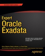
When Linux boots up it runs a scan to identify disks attached to the server. When a disk is found, the O/S determines the device driver needed and creates a block device called a LUN for application access. While it is possible for applications to read and write directly to these block devices, it is not a common practice. Doing so subjects the application to changes that are complicated to deal with. For example, because device names are dynamically generated on bootup, adding or replacing a disk can cause all of the disk device names to change. ASM and databases need file permissions to be set that will allow read/write access to these devices as well. In earlier releases of ASM this was managed by the system administrator through the use of native Linux commands like raw and udev. Exadata shields system administrators and DBAs from these complexities through various layers of abstraction. Cell disks provide the first abstraction layer for LUNs. Cell disks are used by cellsrv to manage I/O resources at the storage cell. Grid disks are the next layer of abstraction and are the disk devices presented to the database servers as ASM Disks. Figure 14-1 shows how cell disks and grid disks fit into the overall storage architecture of an Exadata storage cell.

Figure 14-1. The relationship between physical disks and grid disks

With the introduction of ASM, Oracle provided a way to combine many physical disks into a single storage volume called a disk group. Disk groups are the ASM replacement for traditional file systems and are used to implement Oracle's SAME (Stripe and Mirror Everything) methodology for optimizing disk performance. As the name implies, the goal of SAME is to spread I/O evenly across all physical disks in the storage array. Virtualizing storage in this way allows multiple databases to share the same physical disks. It also allows physical disks to be added or removed without interrupting database operations. If a disk must be removed, ASM automatically migrates its data to the other disks in the disk group before it is dropped. When a disk is added to a disk group, ASM automatically rebalances data from other disks onto the new disk. In a very basic ASM configuration, LUNs are presented to ASM as ASM disks. ASM disks are then used to create disk groups, which in turn are used to store database files such as datafiles, control files, and online redo logs. The Linux operating system presents LUNs to ASM as native block devices such as /dev/sda1. Exadata virtualizes physical storage through the use of grid disks and ASM disk groups. Grid disks are used for carving up cell disks similar to the way partitions are used to carve up physical disk drives. Figure 14-2 shows the relationship between cell disks, grid disks, and ASM disk groups.

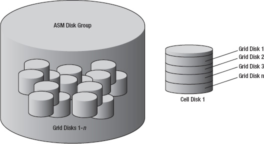
Figure 14-2. ASM disk group with its underlying grid disks, and cell disks

Failure Groups

Before we talk in more detail about grid disks, let's take a brief detour and talk about how disk redundancy is handled in the ASM architecture. ASM uses redundant sets of ASM disks called failure groups to provide mirroring. Traditional RAID0 mirroring maintains a block-for-block duplicate of the original disk. ASM failure groups provide redundancy by assigning ASM disks to failure groups and guaranteeing that the original and mirror copy of a block do not reside within the same failure group. It is critically important to separate physical disks into separate failure groups. Exadata does this by assigning the grid disks from each storage cell to a separate failure groups. For example, the following listing shows the fail groups and grid disks for storage cells 1-3. As the names imply, these fail groups correspond to storage cells 1–3. These fail groups were created and named automatically by ASM when the grid disks were created.

Figure 14-3 shows the relationship between the DATA_DG disk group and the failure groups, CELL01, CELL02, and CELL03. Note that this does not indicate which level of redundancy is being used, only that the DATA_DG disk group has its data allocated across three failure groups.

Figure 14-3. ASM failure groups CELL01 – CELL03

There are three types of redundancy in ASM: External, Normal, and High.

External Redundancy: No redundancy is provided by ASM. It is assumed that the storage array, usually a SAN, is providing adequate redundancy; in most cases RAID0, RAID10, or RAID5. This has become the most common method where large storage area networks are used for ASM storage. In the Exadata storage grid, ASM provides the only mechanism for mirroring. If External Redundancy were used, the loss of a single disk drive would mean a catastrophic loss of all ASM diskgroups using that disk. It also means that even the temporary loss of a storage cell (reboot, crash, or the like) would make all disk groups using storage on the failed cell unavailable for the duration of the outage.

Normal Redundancy: Normal Redundancy maintains two copies of data blocks in separate failure groups. Databases will always attempt to read from the primary copy of a data block first. Secondary copies are only read when the primary blocks are unavailable. At least two failure groups are required for Normal Redundancy, but many more than that may be used. For example, an Exadata full rack configuration has 14 storage cells, and each storage cell constitutes a failure group. When data is written to the database, the failure group used for the primary copy of a block rotates from failure group to failure group in a round-robin fashion. This ensures that disks in all failure groups participate in read operations.

High Redundancy: High Redundancy is similar to Normal Redundancy except that three copies of data blocks are maintained in separate failure groups.

Grid Disks

Grid disks are created within cell disks, which you may recall are made up of physical disks and Flash Cache modules. In a simple configuration one grid disk can be created per cell disk. More complex configurations have multiple grid disks per cell disk. The CellCLI command, list griddisk displays the various characteristics of grid disks. For example, the following output shows the relationship between grid disks and cell disks, the type of device on which they are created, and their size.

ASM doesn't know anything about physical disks or cell disks. Grid disks are what the storage cell presents to the database servers (as ASM disks) to be used for Clusterware and database storage. ASM uses grid disks to create disk groups in the same way conventional block devices are used on a non-Exadata platform. To illustrate this, the following query shows what ASM disks look like on a non-Exadata system.

The same query on Exadata reports grid disks that have been created at the storage cell.

Tying it all together, Figure 14-4 shows how the layers of storage fit together, from the storage cell to the ASM disk group. Note, that the Linux O/S partitions on the first two cell disks in each storage cell are identified by a dotted line. We'll talk a little more about the O/S partitions later in the chapter, and in much more detail in Chapter 8.

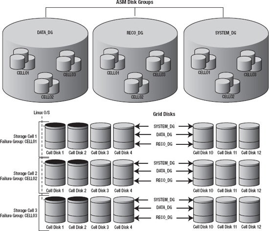
Figure 14-4. Storage virtualization on Exadata

Storage Allocation

Disk drives store data in concentric bands called tracks. Because the outer tracks of a disk have more surface area, they are able to store more data than the inner tracks. As a result, data transfer rates are higher for the outer tracks and decline slightly as you move toward the innermost track. Figure 14-5 shows how tracks are laid out across the disk surface from fastest to slowest.

Figure 14-5. Disk tracks

Exadata provides two policies for allocating grid disk storage across the surface of disk drives. The first method is the default behavior for allocating space on cell disks. It has no official name, so for purposes of this discussion I'll refer to it as the default policy. The other allocation policy Oracle calls interleaving. These two allocation policies are determined when the cell disks are created. Interleaving must be explicitly enabled using the interleaving parameter of the create celldisk command. For a complete discussion on creating cell disks refer to chapter 8.

Fastest Available Tracks First

The default policy simply allocates space starting with the fastest available tracks first, moving inward as space is consumed. Using this policy, the first grid disk created on each cell disk will be given the fastest storage, while the last grid disk created will be relegated to the slower, inner tracks of the disk surface. When planning your storage grid, remember that grid disks are the building blocks for ASM disk groups. These disk groups will in turn be used to store tables, indexes, online redo logs, archived redo logs, and so on. To maximize database performance, frequently accessed objects (such as tables, indexes, and online redo logs) should be stored in the highest priority grid disks. Low priority grid disks should be used for less performance sensitive objects such as database backups, archived redo logs, and flashback logs. Figure 14-6 shows how grid disks are allocated using the default allocation policy.

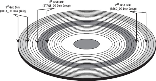
Figure 14-6. The default allocation policy

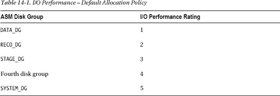
Table 14-1 shows the performance effect on the ASM disk groups from the first to the last grid disk created when using the default allocation policy. You won't find the term “I/O Performance Rating” in the Oracle documentation. It's a term I'm coining here to describe the relative performance capabilities of each disk group due to its location on the surface of the physical disk drive.

Interleaving

The other policy, interleaving, attempts to even out performance of the faster and slower tracks by allocating space in an alternating fashion between the slower and faster tracks of the disks. This is done by splitting each cell disk into two regions, an outer region and an inner region. Grid disks are slices of cell disks that will be used to create ASM disk groups. For example, the following command creates 12 grid disks (one per physical disk; see Figure 14-4) on Cell03 to be used for the DATA_DG disk group:

These grid disks were used to create the following DATA_DG disk group. Notice how each grid disk was created on a separate cell disk:

Using interleaving in this example, DATA_DG_CD_00_CELL03 (the first grid disk) is allocated to the outer most tracks of the outer (fastest) region of the CD_00_CELL03 cell disk. The next grid disk, DATA_DG_CD_01_CELL03, is created on the outermost tracks of the slower, inner region of cell disk CD_01_CELL03. This pattern continues until all 12 grid disks are allocated. When the next set of grid disks is created for the RECO_DG disk group, they start with the inner region of cell disk 1 and alternate from inner to outer region until all 12 grid disks are created. Figure 14-7 shows how the interleaving policy would look if two grid disk groups were created.

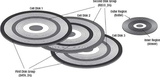
Figure 14-7. The interleaving allocation policy

Table 14-2 shows the performance effect on the ASM disk groups from the first to the last grid disk created when the interleaving allocation policy is used.

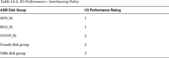
As you can see, the main difference between the default policy and the interleaving policy is that default provides finer-grained control over ASM disks. With the default policy you have the ability to choose which set of grid disks will be given the absolute fastest position on the disk. The interleaving policy has the effect of evening out the performance of grid disks. In practice, this gives the first two sets of grid disks (for DATA_DG and RECO_DG) the same performance characteristics. This may be useful if the performance demands of the first two disk groups are equal. In our experience this is rarely the case. Usually there is a clear winner when it comes to the performance demands of a database environment. Tables, indexes, online redo logs (the DATA_DG disk group) have much higher performance requirements than database backups, archived redo logs, and flashback logs, which are usually stored in the RECO disk group. Unless there are specific reasons for using interleaving, we recommend using the default policy.

Creating Grid Disks

Before we run through a few examples of how to create grid disks, let's take a quick look at some of their key attributes:

• Multiple grid disks may be created on a single cell disk, but a grid disk may not span multiple cell disks.
• Storage for grid disks is allocated in 16M Allocation Units (AUs) and is rounded down if the size requested is not a multiple of the AU size.
• Grid disks may be created one at a time or in groups with a common name prefix.
• Grid disk names must be unique within a storage cell and should be unique across all storage cells.
• Grid disk names should include the name of the cell disk on which they reside.

Once a grid disk is created, its name is visible from ASM in the V$ASM_DISK view. In other words, grid disks = ASM disks. It is very important to name grid disks in such a way that they can easily be associated with the physical disk to which they belong in the event of disk failure. To facilitate this, grid disk names should include both of the following:

• The name of the ASM disk group for which it will be used
• The cell disk name (which includes the name of the storage cell)

Figure 14-8 shows the properly formatted name for a grid disk belonging to the TEST_DG disk group, created on cell disk CD_00_cell03.

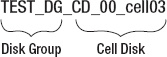
Figure 14-8. Grid disk naming

Creating Grid Disks

The CellCLI command create griddisk is used to create grid disks. It may be used to create individual grid disks one at a time or in groups. If grid disks are created one at a time, it is up to you to provide the complete grid disk name. The following example creates one properly named 96 MB grid disk on cell disk CD_00_cell03. If we had omitted the size=100M parameter, the resulting grid disk would have consumed all free space on the cell disk.

There are 12 drives per storage cell, and the number of storage cells varies from 3, for a quarter rack, to 14, for a full rack. That means you will be creating a minimum of 36 grid disks for a quarter rack, and up to 168 grid disks for a full rack. Fortunately, CellCLI provides a way to create all the grid disks needed for a given ASM disk group in one command. For example, the following command creates all the grid disks for the ASM disk group TEST_DG:

When this variant of the create griddisk command is used, CellCLI automatically creates one grid disk on each cell disk, naming them with the prefix you provided in the following manner:

The optional size parameter specifies the size of each individual grid disk. If no size is provided, the resulting grid disks will consume all remaining free space of their respective cell disk. The all harddisk parameter instructs CellCLI to use only disk-based cell disks. Just in case you are wondering, Flash Cache modules are also presented as cell disks (of type FlashDisk) and may be used for creating grid disks as well. We'll discuss flash disks later on in this chapter. The following command shows the grid disks created.

Grid Disk Sizing

As we discussed earlier, grid disks are equivalent to ASM disks. They are literally the building blocks of the ASM disk groups you will create. The SYSTEM_DG disk group is created when Exadata is installed on a site. It is primarily used to store the OCR and voting files used by Oracle clusterware (Grid Infrastructure). However, there is no reason SYSTEM_DG cannot be used to store other objects such as tablespaces for the Database File System (DBFS). In addition to the SYSTEM_DG, (or DBFS_DG) disk group, Exadata is also delivered with DATA and RECO disk groups to be used for database files and Fast Recovery Areas. But these disk groups may actually be created with whatever names make the most sense for your environment. For consistency, this chapter uses the names SYSTEM_DG, DATA_DG and RECO_DG. If you are considering something other than the “factory defaults” for your disk group configuration, remember that a main reason for using multiple ASM disk groups on Exadata is to prioritize I/O performance. The first grid disks you create will be the fastest, resulting in higher performance for the associated ASM disk group.

By the way, Oracle recommends you create a separate database for DBFS because it requires instance parameter settings that would not be optimal for typical application databases.

Some of the most common ASM disk groups are

SYSTEM_DG: This disk group is the location for clusterware's OCR and voting files. It may also be used for other files with similar performance requirements. For OCR and voting files, normal redundancy is the minimum requirement. Normal redundancy will create 3 voting files, and 3 OCR files. The voting files must be stored is separate ASM failure groups. Recall that on Exadata, each storage cell constitutes a failure group. This means that only normal redundancy may be used for an Exadata quarter rack configuration (3 storage cells/failure groups). Only in half rack and full rack configurations (7 or 14 storage cells/failure groups), are there a sufficient number of failure groups to store the required number of voting and OCR files required by high redundancy. Table 14-3 summarizes the storage requirements for OCR and voting files at various levels of redundancy. Note that External Redundancy is not supported on Exadata. We've included it in the table for reference only.

DATA_DG: This disk group is used for storing files associated with the db_create_file_dest database parameter. These include datafiles, online redo logs, control files, and spfiles.

RECO_DG: This disk group is what used to be called Flash Recovery Area (FRA). Sometime after 11gR1 Oracle renamed it to the “Fast Recovery Area”; rumor has it that the overuse of “Flash” was causing confusion among the marketing team. So to clarify, this diskgroup will be used to store everything corresponding to the db_recovery_file_dest database parameter. It includes online database backups and copies, mirror copies of the online redo log files, mirror copies of the control file, archived redo logs, flashback logs, and Data Pump exports.

Recall that Exadata storage cells are actually finely tuned Linux servers with 12 internal disk drives. Oracle could have dedicated two of these internal disks to run the operating system, but doing so would have wasted a lot of space. Instead, they carved off several small partitions on the first two disks in the enclosure. These partitions, about 30 GB each, create a slight imbalance in the size of the cell disks. This imbalance is so small it doesn't affect performance, but it is something that you will have to work with when planning your grid disk allocation strategy. Figure 14-9 illustrates this imbalance.

Figure 14-9. Cell disk layout

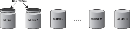
This reserved space can be seen by running fdisk on one of the storage cells. The /dev/sda3 partition in the listing is the location of the cell disk. All other partitions are used by the Linux operating system.

You can see the smaller cell disks in the size attribute when you run the list celldisk command:

Let's take a look at a fairly typical configuration to illustrate how grid disks are allocated in the storage cell. In this example we'll create grid disks to support three ASM disk groups. SYSTEM_DG is fairly large and will be used for DBFS (clustered file system storage) in addition to the OCR and Voting files.

• DATA_DG
• RECO_DG
• SYSTEM_DG

This storage cell is configured with SATA disks, so the total space per storage cell is 21.76 terabytes. Table 14-4 shows what the allocation would look like. In all cases the physical disk size is 1,861.703125. The sum of the disk sizes is then 22,340.437500.

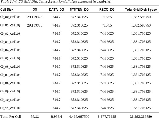
Creating a configuration like this is fairly simple. The following commands create grid disks according to the allocation in Table 14-4.

Notice that no size was specified for the RECO_DG grid disks. When size is not specified, CellCLI automatically calculates the size for each grid disk so they consume the remaining free space on the cell disk. For example:

Creating FlashDisk-Based Grid Disks

Exadata uses offloading features like Smart Scan to provide strikingly fast I/O for direct path reads typically found in DSS databases. These features are only activated for very specific data access paths in the database. To speed up I/O performance for random reads, Exadata V2 introduced solid-state storage called Flash Cache. Each storage cell comes configured with four 96G Flash Cache cards (366G usable) to augment I/O performance for frequently accessed data. When configured as Exadata Smart Flash Cache, these devices act like a large, database-aware disk cache for the storage cell. We discussed this in detail in Chapter 5. Optionally, some space from the Flash Cache may be carved out and used like high-speed, solid-state disks. Flash Cache is configured as a cell disk of type FlashDisk, and just as grid disks are created on HardDisk cell disks, they may also be created on FlashDisk cell disks. When FlashDisks are used for database storage, it's primarily to improve performance for highly write-intensive workloads when disk-based storage cannot keep up. FlashDisk cell disks may be seen using the CellCLI list celldisk command, as in the following example:

FlashDisk type cell disks are named with a prefix of FD and a diskType of FlashDisk. It is not recommended to use all of your Flash Cache for grid disks. When creating the Flash Cache, use the size parameter to hold back some space to be used for grid disks. The following command creates a Flash Cache of 300GB, reserving 65GB (4.078125GB × 16) for grid disks:

Note that the create flashcache command uses the size parameter differently than the create griddisk command. When creating the flash cache, the size parameter determines the total size of the cache.

Now we can create 16 grid disks using the remaining free space on the Flash Disks, using the familiar create griddisk command. This time we'll specify flashdisk for the cell disks to use:

Once the grid disks have been created they may be used to create ASM disk groups used to store database objects just as you would any other disk-based disk group. The beauty of Flash Cache configuration is that all this may be done while the system is online and servicing I/O requests. All of the commands we've just used to drop and reconfigure the Flash Cache were done without the need to disable or shutdown databases or cell services.

Storage Strategies

Each Exadata storage cell is an intelligent mini-SAN, operating somewhat independently of the other cells in the rack. Now this may be stretching the definition of SAN a little, but with the Cell Server software intelligently controlling I/O access we believe it is appropriate. Storage cells may be configured in such a way that all Cells in the rack provide storage for all databases in the rack. This provides maximum I/O performance and data transfer rates for each database in the system. Storage cells may also be configured to service specific database servers using the cellip.ora file. In addition, cell security may be used to restrict access to specific databases or ASM instances through use of storage realms. In this section I'll discuss strategies for separating cells into groups that service certain database servers or RAC clusters. To borrow a familiar term from the SAN world, this is where we will talk about “zoning” a set of storage cells to service development, test, and production environments.

Configuration Options

Exadata represents a substantial investment for most companies. For one reason or another, we find that many companies want to buy a full or half rack for consolidating several database environments. Exadata's architecture makes it a very good consolidation platform. These are some of the most common configurations we've seen:

• A full rack servicing development, test, and production
• A full rack servicing several, independent production environments
• A half rack servicing development and test
• Isolating a scratch environment for DBA testing and deploying software patches

For each of these configurations, isolating I/O to specific database servers may be a key consideration. For example, your company may be hosting database environments for external clients that require separation from other database systems. Or your company may have legal requirements to separate server access to data. Another reason for segmenting storage at the cell level may be to provide an environment for DBA training, or testing software patches. There are two ways to isolate Exadata storage cells, by network access and by storage realm.

Isolating Storage Cell Access

Recall that ASM gains access to grid disks through the Infiniband network. This is configured by adding the IP address of storage cells in the cellip.ora file. For example, in a full rack configuration, all 14 storage cells are listed as follows:

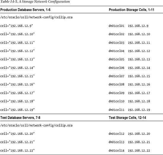
When ASM starts up it interrogates the storage cells on each of these IP addresses for grid disks it can use for configuring ASM disk groups. We can easily segregate storage cells to service specific database servers by removing the IP address of cells that should not be used. Obviously this is not enforced by any kind of security but it is an effective, simple way of pairing up database servers with the storage cells they should use for storage. Table 14-5 illustrates a configuration that splits a full rack into two database, and storage grids. Production is configured with six database servers and 11 storage cells, while Test is configured for two database servers and three storage cells.

Database servers and storage cells can be paired in any combination that best suits your specific needs. Remember that the minimum requirements for Oracle RAC on Exadata requires two database servers and three storage cells, which is basically a quarter rack configuration. Table 14-6 shows the storage and performance capabilities of Exadata storage cells in quarter rack, half rack, and full rack configurations.

If some of your environments do not require Oracle RAC, there is no reason they cannot be configured with stand alone (non-RAC) database servers. If this is done, then a minimum of one storage cell may be used to provide database storage for each database server. In fact a single storage cell may even be shared by multiple standalone database servers. Once again, Exadata is a highly configurable system. But just because you can do something, doesn't mean you should. Storage cells are the workhorse of Exadata. Each cell supports a finite data transfer rate (MBPS) and number of I/O's per second (IOPS). Reducing the storage cell footprint of your database environment directly impacts the performance your database can yield

Cell Security

In addition to isolating storage cells by their network address, Exadata also provides a way to secure access to specific grid disks within the storage cell. An access control list (ACL) is maintained at the storage cell, and grid disks are defined as being accessible to specific ASM clusters and, optionally, databases within the ASM cluster. If you've already logged some time working on your Exadata system, chances are you haven't noticed any such access restrictions. That is because by default, cell security is open, allowing all ASM clusters and databases in the system access to all grid disks. Cell security controls access to grid disks at two levels, by ASM cluster and by database:

ASM-Scoped Security: ASM-scoped security restricts access to grid disks by ASM cluster. This is the first layer of cell security. It allows all databases in the ASM cluster to have access to all grid disks managed by the ASM instance. For example, an Exadata full rack configuration can be split so that four database servers and seven storage cells can be used by Customer-A, and the other four database servers and seven storage cells can be used by Customer-B.

Database-Scoped Security: Once ASM-scoped security is configured, access to grid disks may be further controlled at the database level using database-scoped security. Database-scoped security is most appropriate when databases within the ASM cluster should have access to a subset of the grid disks managed by the ASM instance. In the earlier example Customer-A's environment could use database-scoped security to separate database environments from one another within its half rack configuration.

Cell Security Terminology

Before we get too far along, let's take a look at some of the new terminology specific to Exadata's cell security.

Storage Realm: Grid disks that share a common security domain are referred to as a storage realm.

Security Key: A security key is used to authenticate ASM and database clients to the storage realm. It is also used for securing messages sent between the storage cells and the ASM and database clients. The security key is created using the CellCLI command create key. The key is then assigned to grid disks using the CellCLI assign key command.

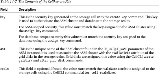
cellkey.ora: The cellkey.ora file is stored on the database servers. One cellkey.ora file is created for ASM-scoped security and another cellkey.ora file is created for each database requiring database-scoped security. The cellkey.ora files are used to identify security keys, the storage realm, and the unique name of the ASM cluster or database.

Table 14-7 shows the definitions for the fields in the cellkey.ora file.

Cell Security Best Practices

Following Oracle's best practices is an important part of configuring cell security. It will help you avoid those odd situations where things seem to work some of the time or only on certain storage cells. Following these best practices will save you a lot of time and frustration:

• If database-scoped security is used, be sure to use it for all databases in the ASM cluster.
• Make sure the ASM cellkey.ora file is the same on all servers for an ASM cluster. This includes contents, ownership, and permissions.
• Just as you did for the ASM cellkey.ora file, make sure contents, ownership, and permissions are identical across all servers for the database cellkey.ora file.
• Ensure the cell side security settings are the same for all grid disks belonging to the same ASM disk group.
• It is very important that the cellkey.ora files and cell commands are executed consistently across all servers and cells. Use the dcli utility to distribute the cellkey.ora file and reduce the likelihood of human error.

Configuring ASM-Scoped Security

With ASM-scoped security, the ASM cluster is authenticated to the storage cell by its DB_UNIQUE_NAME and a security key. The security key is created at the storage cell and stored in the cellkey.ora file on the database server. An access control list (ACL) is defined on the storage cell that is used to verify the security key it receives from ASM. The availableTo attribute on each grid disk dictates which ASM clusters are permitted access.

Now let's take a look at the steps for configuring ASM-scoped security.

1. Shut down all databases and ASM instances in the ASM cluster.
2. Create the security key using the CellCLI create key command:
   CellCLI> create key
        3648e2a3070169095b799c44f02fea9

   This simply generates the key, which is not automatically stored anywhere. The create key command only needs to be run once and can be done on any storage cell. This security key will be assigned to the ASM cluster in the key field of the cellkey.ora file.

3. Next, create a cellkey.ora file and install it in the /etc/oracle/cell/network-config directory for each database server on which this ASM cluster is configured. Set the ownership of the file to the user and group specified during the ASM software installation. Permissions should allow it to be read by the user and group owner of the file. For example:
   key=3648e2a3070169095b799c44f02fea9
asm=+ASM
realm=customer_A_realm

> chown oracle:dba cellkey.ora
> chmod 640 cellkey.ora

   Note that if a realm is defined in this file it must match the realm name assigned to the storage cells using the alter cell realm= command.

4. Find the DB_UNIQUE_NAME for your ASM cluster using the show parameter command from one of the ASM instances:
   SYS:+ASM1>show parameter db_unique_name

NAME             TYPE        VALUE
---------------- ----------- ------------------
db_unique_name   string      +ASM
5. Use the CellCLI assign key command to assign the security key to the ASM cluster being configured. This must be done on each storage cell to which you want the ASM cluster to have access:
   CellCLI> ASSIGN KEY -
            FOR '+ASM='66e12adb996805358bf82258587f5050'
6. Using the CellCLI create griddisk command, set the availableTo attribute for each grid disk to which you want this ASM cluster to have access. This can be done for all grid disks on the cell as follows:
   CellCLI> create griddisk all prefix='DATA_DG' -
                size= 1282.8125G availableTo='+ASM'
7. For existing grid disks, use the alter grid disk command to set up security:
   CellCLI> alter griddisk all prefix='DATA_DG' -
               availableTo='+ASM'
8. A subset of grid disks may also be assigned, as follows:
   CellCLI> alter griddisk DATA_CD_00_cell03, -
                        DATA_CD_01_cell03, -
                        DATA_CD_02_cell03, -
                        ...
               availableTo='+ASM'

This completes the configuration of ASM-scoped cell security. The ASM cluster and all databases can now be restarted. When ASM starts up it will check for the cellkey.ora file and pass the key to the storage cells in order to gain access to the grid disks.

Configuring Database-Scoped Security

Database-scoped security locks down database access to specific grid disks within an ASM cluster. It is useful for controlling access to grid disks when multiple databases share the same ASM cluster. Before database-scoped security may be implemented, ASM-scoped security must be configured and verified.

When using database-scoped security, there will be one cellkey.ora file per database, per database server, and one ACL entry on the storage cell for each database. The following steps may be used to implement simple database-scoped security for two databases, called HR (Human Resources) and PAY (Payroll)).

1. Shut down all databases and ASM instances in the ASM cluster.
2. Create the security key using the CellCLI create key command:
   CellCLI> create key
        7548a7d1abffadfef95a53185aba0e98

CellCLI> create key
        8e7105bdbd6ad9fa53d41736a533b9b1

   The create key command must be run once for each database in the ASM cluster. It can be run from any storage cell. One security key will be assigned to each database within the ASM cluster in the key field of the database cellkey.ora file.

3. For each database, create a cellkey.ora file using the keys created in step 2. Install these cellkey.ora files in the ORACLE_HOME/admin/{db_unique_name}/pfile directories for each database server on which database-scoped security will be configured. Just as you did for ASM-scoped security, set the ownership of the file to the user and group specified during the ASM software installation. Permissions should allow it to be read by the user and group owner of the file. For example:
   # -- Cellkey.ora file for the HR database --#
key=7548a7d1abffadfef95a53185aba0e98
asm=+ASM
realm=customer_A_realm
# --

> chown oracle:dba $ORACLE_HOME/admin/HR/cellkey.ora
> chmod 640 $ORACLE_HOME/admin/HR/cellkey.ora

# -- Cellkey.ora file for the PAY database --#
key=8e7105bdbd6ad9fa53d41736a533b9b1
asm=+ASM
realm=customer_A_realm
# --

> chown oracle:dba $ORACLE_HOME/admin/PAY/cellkey.ora
> chmod 640 $ORACLE_HOME/admin/PAY/cellkey.ora

   Note that if a realm is defined in this file, it must match the realm name assigned to the storage cells using the alter cell realm= command.

4. Retrieve the DB_UNIQUE_NAME for each database being configured using the show parameter command from each of the databases:
   SYS:+HR>show parameter db_unique_name

NAME             TYPE        VALUE
---------------- ----------- ------------------
db_unique_name   string      HR


SYS:+PAY>show parameter db_unique_name

NAME             TYPE        VALUE
---------------- ----------- ------------------
db_unique_name   string      PAY
5. Use the CellCLI assign key command to assign the security keys for each database being configured. This must be done on each storage cell you want the HR and PAY databases to have access to. The following keys are assigned to the DB_UNIQUE_NAME of the )HR and ))PAY databases:
   CellCLI> ASSIGN KEY -
   FOR HR='7548a7d1abffadfef95a53185aba0e98', –
      PAY='8e7105bdbd6ad9fa53d41736a533b9b1'  –

Key for HR successfully created
Key for PAY successfully created
6. Verify that the keys were assigned properly:
   CellCLI> list key
         HR      d346792d6adea671d8f33b54c30f1de6
         PAY     cae17e8fdce7511cc02eb7375f5443a8
7. Using the CellCLI create disk or alter griddisk command, assign access to the grid disks to each database. Note that the ASM unique name is included with the database unique name in this assignment.
   CellCLI> create griddisk DATA_CD_00_cell03, -
                         DATA_CD_01_cell03  -
                size=1282.8125G             -
                availableTo='+ASM,HR'

CellCLI> create griddisk DATA_CD_02_cell03, -
                         DATA_CD_03_cell03  -
                size=1282.8125G             -
                availableTo='+ASM,PAY'
8. The alter griddisk command may be used to change security assignments for grid disks. For example:
   CellCLI> alter griddisk DATA_CD_05_cell03, -
                        DATA_CD_06_cell03  -
               availableTo='+ASM,HR'

CellCLI> alter griddisk DATA_CD_01_cell03, -
                        DATA_CD_02_cell03  -
               availableTo='+ASM,PAY'

This completes the configuration of database-scoped security for the HR and PAY databases. The ASM cluster and databases may now be restarted. The human resources database now has access to the DATA_CD_00_cell03 and DATA_CD_01_cell03 grid disks, while the payroll database has access to the DATA_CD_02_cell03 and DATA_CD_03_cell03 grid disks.

Removing Cell Security

Once implemented, cell security may be modified as needed by updating the ACL lists on the storage cells, and changing the availableTo attribute of the grid disks. Removing cell security is a fairly straightforward process of backing out the database security settings and then removing the ASM security settings.

The first step in removing cell security is to remove database-scoped security. The following steps will remove database-scoped security from the system.

1. Before database security may be removed, the databases and ASM cluster must be shut down.
2. Remove the databases from the availableTo attribute of the grid disks using the CellCLI command alter griddisk. This command doesn't selectively remove databases from the list. It simply redefines the complete list. Notice that we will just be removing the databases from the list at this point. The ASM unique name should remain in the list for now. This must be done for each cell you want to remove security from.
   CellCLI> alter griddisk DATA_CD_00_cell03, -
                        DATA_CD_01_cell03  -
               availableTo='+ASM'

CellCLI> alter griddisk DATA_CD_02_cell03, -
                        DATA_CD_03_cell03  -
               availableTo='+ASM'

   Optionally, all the databases may be removed from the secured grid disks with the following command:

   CellCLI> alter griddisk DATA_CD_00_cell03, -
                        DATA_CD_01_cell03  -
                        DATA_CD_02_cell03  -
                        DATA_CD_03_cell03  -
               availableTo='+ASM'

   Assuming that these databases have not been configured for cell security on any other grid disks in the cell, the security key may be removed from the ACL list on the storage cell as follows:

   CellCLI> assign key for HR='', PAY=''

Key for HR successfully dropped
Key for PAY successfully dropped
3. Remove the cellkey.ora file located in the ORACLE_HOME/admin/{db_unique_name}/pfile directory for the database client.
4. Now the cellkey.ora file for the HR and PAY databases may be removed from the database servers.
   > rm $ORACLE_HOME/admin/HR/cellkey.ora
> rm $ORACLE_HOME/admin/PAY/cellkey.ora
5. Verify that the HR and PAY databases are not assigned to any grid disks with the following CellCLI command:
   CellCLI> list griddisk attributes name, availableTo

Once database-scoped security has been removed, you can remove ASM-scoped security. This will return the system to open security status. The following steps remove ASM-scoped security. Once this is done, the grid disks will be available to all ASM clusters and databases on the storage network.

1. Before continuing with this procedure, be sure that database-scoped security has been completely removed. The list key command should display the key assignment for the ASM cluster only. No databases should be assigned keys at this point. The list griddisk command should show all the names of the grid disks assignments for the ASM cluster, '+ASM'.
   CellCLI> list griddisk attributes name, availableTo
2. Next, remove the ASM unique name from the availableTo attribute on all grid disks.
   CellCLI> list griddisk attributes name, availableTo
3. Now, remove the ASM security from the ACL by running the following command.
   CellCLI> alter griddisk all assignTo=''
4. The following command removes the ASM cluster assignment for select grid disks:
   CellCLI> alter griddisk DATA_CD_00_cell03, -
                        DATA_CD_01_cell03  -
                        DATA_CD_02_cell03  -
                        DATA_CD_03_cell03  -
               availableTo=''
5. The list griddisk command should show no assigned clients. Verify this by running the list griddisk command.
6. The ASM cluster key may now be safely removed from the storage cell using the CellCLI assign key command:
   CellCLI> list key detail
         name:     +ASM
         key:      196d7983a9a33fccae276e24e7a9f89

CellCassign key for +ASM=''
Key for +ASM successfully dropped
7. Remove the cellkey.ora file from the /etc/oracle/cell/network-config directory on all database servers in the ASM cluster.

This completes the removal of ASM-scoped security. The ASM cluster may now be restarted as well as all the databases it services.

Summary

Understanding all the various layers of the Exadata storage architecture and how they fit together is a key component to properly laying out storage for databases. Understanding the relationship between physical disks, LUNs, cell disks, grid disks, and ASM disk groups is absolutely necessary if you want to carve up disk storage for maximum performance. In this chapter we've discussed what grid disks are, what they are made up of, and how they fit into the ASM storage grid. We've taken a look at how to create disk groups so that IO is prioritized for performance critical datafiles. Carving up storage doesn't end at the disk, so we also discussed methods for partitioning storage by cell and by grid disk within the cell.