Chapter 20

Efficient Shading

For simple scenes—relatively little geometry, basic materials, a few lights—we can use the standard GPU pipeline to render images without concerns about maintaining frame rate. Only when one or more elements become expensive do we need to use more involved techniques to rein in costs. In the previous chapter we focused on culling triangles and meshes from processing further downstream. Here we concentrate on techniques for reducing costs when evaluating materials and lights. For many of these methods, there is an additional processing cost, with the hope being that this expense is made up by the savings obtained. Others trade off between bandwidth and computation, often shifting the bottleneck. As with all such schemes, which is best depends on your hardware, scene structure, and many other factors.

Evaluating a pixel shader for a material can be expensive. This cost can be reduced by various shader level of detail simplification techniques, as noted in Section 19.9. When there are several light sources affecting a surface, two different strategies can be used. One is to build a shader that supports multiple light sources, so that only a single pass is needed. Another is multi-pass shading, where we create a simple one-light pixel shader for a light and evaluate it, adding each result to the framebuffer. So, for three lights, we would draw the primitive three times, changing the light for each evaluation. This second method might be more efficient overall than a single-pass system, because each shader used is simpler and faster. If a renderer has many different types of lights, a one-pass pixel shader must include them all and test for whether each is used, making for a complex shader.

In Section 18.4.5 we discussed avoiding unnecessary pixel shader evaluations by minimizing or eliminating overdraw. If we can efficiently determine that a surface does not contribute to the final image, then we can save the time spent shading it. One technique performs a z-prepass, where the opaque geometry is rendered and only z-depths are written. The geometry is then rendered again fully shaded, and the z-buffer from the first pass culls away all fragments that are not visible. This type of pass is an attempt to decouple the process of finding what geometry is visible from the operation of subsequently shading that geometry. This idea of separating these two processes is an important concept used throughout this chapter, and is employed by several alternative rendering schemes.

For example, a problem with using a z-prepass is that you have to render the geometry twice. This is an additional expense compared to standard rendering, and could cost more time than it saves. If the meshes are formed via tessellation, skinning, or some other involved process, the cost of this added pass can be considerable [992, 1177]. Objects with cutout alpha values need to have their texture’s alpha retrieved each pass, adding to the expense, or must be ignored altogether and rendered only in the second pass, risking wasted pixel shader evaluations. For these reasons, sometimes only large occluders (in screen or world space) are drawn in this initial pass. Performing a full prepass may also be needed by other screen-space effects, such as ambient occlusion or reflection [1393]. Some of the acceleration techniques presented in this chapter require an accurate z-prepass that is then used to help cull lists of lights.

Even with no overdraw, a significant expense can arise from a large number of dynamic lights evaluated for a visible surface. Say you have 50 light sources in a scene. A multi-pass system can render the scene successfully, but at the cost of 50 vertex and shader passes per object. One technique to reduce costs is to limit the effect of each local light to a sphere of some radius, cone of some height, or other limited shape [668, 669, 1762, 1809]. The assumption is that each light’s contribution becomes insignificant past a certain distance. For the rest of this chapter, we will refer to lights’ volumes as spheres, with the understanding that other shapes can be used. Often the light’s intensity is used as the sole factor determining its radius. Karis [860] discusses how the presence of glossy specular materials will increase this radius, since such surfaces are more noticeably affected by lights. For extremely smooth surfaces this distance may go to infinity, such that environment maps or other techniques may need to be used instead.

A simple preprocess is to create for each mesh a list of lights that affects it. We can think of this process as performing collision detection between a mesh and the lights, finding those that may overlap [992]. When shading the mesh, we use this list of lights, thus reducing the number of lights applied. There are problems with this type of approach. If objects or lights move, these changes affect the composition of the lists. For performance, geometry sharing the same material is often consolidated into larger meshes (Section 18.4.2), which could cause a single mesh to have some or all of the lights in a scene in its list [1327, 1330]. That said, meshes can be consolidated and then split spatially to provide shorter lists [1393].

Another approach is to bake static lights into world-space data structures. For example, in the lighting system for Just Cause 2, a world-space top-down grid stores light information for a scene. A grid cell represents a 4 meter 4 meter area. Each cell is stored as a texel in an RGBα texture, thus holding a list of up to four lights. When a pixel is rendered, the list in its area is retrieved and the relevant lights are applied [1379]. A drawback is that there is a fixed storage limit to the number of lights affecting a given area. While potentially useful for carefully designed outdoor scenes, buildings with a number of stories can quickly overwhelm this storage scheme.

Our goal is to handle dynamic meshes and lights in an efficient way. Also important is predictable performance, where a small change in the view or scene does not cause a large change in the cost of rendering it. Some levels in DOOM (2016) have 300 visible lights [1682]; some scenes in Ashes of the Singularity have 10,000. See Figure 20.1 and Figure 20.15 on page 913. In some renderers a large number of particles can each be treated as small light sources. Other techniques use light probes (Section 11.5.4) to illuminate nearby surfaces, which can be thought of as short-range light sources.

20.1 Deferred Shading

So far throughout this book we have described forward shading, where each triangle is sent down the pipeline and, at the end of its travels, the image on the screen is updated with its shaded values. The idea behind deferred shading is to perform all visibility testing and surface property evaluations before performing any material lighting computations. The concept was first introduced in a hardware architecture in 1988 [339], later included as a part of the experimental PixelFlow system [1235], and used as an offline software solution to help produce non-photoreal styles via image processing [1528]. Calver’s extensive article [222] in mid-2003 lays out the basic ideas of using deferred shading on the GPU. Hargreaves and Harris [668, 669] and Thibieroz [1762] promoted its use the following year, at a time when the ability to write to multiple render targets was becoming more widely available.

In forward shading we perform a single pass using a shader and a mesh representing the object to compute the final image. The pass fetches material properties— constants, interpolated parameters, or values in textures—then applies a set of lights to these values. The z-prepass method for forward rendering can be seen as a mild decoupling of geometry rendering and shading, in that a first geometry pass aims at only determining visibility, while all shading work, including material parameter retrieval, is deferred to a second geometry pass performed to shade all visible pixels. For interactive rendering, deferred shading specifically means that all material parameters associated with the visible objects are generated and stored by an initial geometry pass, then lights are applied to these stored surface values using a post-process. Values saved in this first pass include the position (stored as z-depth), normal, texture coordinates, and various material parameters. This pass establishes all geometry and material information for the pixel, so the objects are no longer needed, i.e., the contribution of the models’ geometry has been fully decoupled from lighting computations. Note that overdraw can happen in this initial pass, the difference being that the shader’s execution is considerably less—transferring values to buffers—than that of evaluating the effect of a set of lights on the material. There is also less of the additional cost found in forward shading, where sometimes not all the pixels in a 2 2 quad are inside a triangle’s boundaries but all must be fully shaded [1393] (Section 23.8). This sounds like a minor effect, but imagine a mesh where each triangle covers a single pixel. Four fully shaded samples will be generated and three of these discarded with forward shading. Using deferred shading, each shader invocation is less expensive, so discarded samples have a considerably lower impact.

The buffers used to store surface properties are commonly called G-buffers [1528], short for “geometric buffers.” Such buffers are also occasionally called deep buffers, though this term can also mean a buffer storing multiple surfaces (fragments) per pixel, so we avoid it here. Figure 20.2 shows the typical contents of some G-buffers. A G-buffer can store anything a programmer wants it to contain, i.e., whatever is needed to complete the required subsequent lighting computations. Each G-buffer is a separate render target. Typically three to five render targets are used as G-buffers, but systems have gone as high as eight [134]. Having more targets uses more bandwidth, which increases the chance that this buffer is the bottleneck.

After the pass creating the G-buffers, a separate process is used to compute the effect of illumination. One method is to apply each light one by one, using the G- buffers to compute its effect. For each light we draw a screen-filling quadrilateral (Section 12.1) and access the G-buffers as textures [222, 1762]. At each pixel we can determine the location of the closest surface and whether it is in range of the light. If it is, we compute the effect of the light and place the result in an output buffer. We do this for each light in turn, adding its contribution via blending. At the end, we have all lights’ contributions applied.

This process is about the most inefficient way to use G-buffers, since every stored pixel is accessed for every light, similar to how basic forward rendering applies all lights to all surface fragments. Such an approach can end up being slower than forward shading, due to the extra cost of writing and reading the G-buffers [471]. As a start on improving performance, we could determine the screen bounds of a light volume (a sphere) and use them to draw a screen-space quadrilateral that covers a smaller part of the image [222, 1420, 1766]. In this way, pixel processing is reduced, often significantly. Drawing an ellipse representing the sphere can further trim pixel processing that is outside the light’s volume [1122]. We can also use the third screen dimension, z-depth. By drawing a rough sphere mesh encompassing the volume, we can trim the sphere’s area of effect further still [222]. For example, if the sphere is hidden by the depth buffer, the light’s volume is behind the closest surface and so has no effect. To generalize, if a sphere’s minimum and maximum depths at a pixel do not overlap the closest surface, the light cannot affect this pixel. Hargreaves [668] and Valient [1809] discuss various options and caveats for efficiently and correctly determining this overlap, along with other optimizations. We will see this idea of testing for depth overlap between the surface and the light used in several of the algorithms ahead. Which is most efficient depends on the circumstances.

For traditional forward rendering, the vertex and pixel shader programs retrieve each light’s and material’s parameters and compute the effect of one on the other. Forward shading needs either one complex vertex and pixel shader that covers all possible combinations of materials and lights, or shorter, specialized shaders that handle specific combinations. Long shaders with dynamic branches often run considerably more slowly [414], so a large number of smaller shaders can be more efficient, but also require more work to generate and manage. Since all shading functions are done in a single pass with forward shading, it is more likely that the shader will need to change when the next object is rendered, leading to inefficiency from swapping shaders (Section 18.4.2).

The deferred shading method of rendering allows a strong separation between lighting and material definition. Each shader is focused on parameter extraction or lighting, but not both. Shorter shaders run faster, both due to length and the ability to optimize them. The number of registers used in a shader determines occupancy (Section 23.3), a key factor in how many shader instances can be run in parallel. This decoupling of lighting and material also simplifies shader system management. For example, this split makes experimentation easy, as only one new shader needs to be added to the system for a new light or material type, instead of one for each combination [222, 927]. This is possible since material evaluations are done in the first pass, and lighting is then applied to this stored set of surface parameters in the second pass.

For single-pass forward rendering, all shadow maps usually must be available at the same time, since all lights are evaluated at once. With each light handled fully in a single pass, deferred shading permits having only one shadow map in memory at a time [1809]. However, this advantage disappears with the more complex light assignment schemes we cover later, as lights are evaluated in groups [1332, 1387].

Basic deferred shading supports just a single material shader with a fixed set of parameters, which constrains what material models can be portrayed. One way to support different material descriptions is to store a material ID or mask per pixel in some given field. The shader can then perform different computations based on the G-buffer contents. This approach could also modify what is stored in the G-buffers, based on this ID or mask value [414, 667, 992, 1064]. For example, one material might use 32 bits to store a second layer color and blend factor in a G-buffer, while another may use these same bits to store two tangent vectors that it requires. These schemes entail using more complex shaders, which can have performance implications.

Basic deferred shading has some other drawbacks. G-buffer video memory requirements can be significant, as can the related bandwidth costs in repeatedly accessing these buffers [856, 927, 1766]. We can mitigate these costs by storing lower-precision values or compressing the data [1680, 1809]. An example is shown in Figure 20.3. In Section 16.6 we discussed compression of world-space data for meshes. G-buffers can contain values that are in world-space or screen-space coordinates, depending on the needs of the rendering engine. Pesce [1394] discusses the trade-offs in compressing screen-space versus world-space normals for G-buffers and provides pointers to related resources. A world-space octahedral mapping for normals is a common solution, due to its high precision and quick encoding and decoding times.

Two important technical limitations of deferred shading involve transparency and antialiasing. Transparency is not supported in a basic deferred shading system, since we can store only one surface per pixel. One solution is to use forward rendering for transparent objects after the opaque surfaces are rendered with deferred shading. For early deferred systems this meant that all lights in a scene had to be applied to each transparent object, a costly process, or other simplifications had to be performed. As we will explore in the sections ahead, improved GPU capabilities have led to the development of methods that cull lights for both deferred and forward shading. While it is possible to now store lists of transparent surfaces for pixels [1575] and use a pure deferred approach, the norm is to mix deferred and forward shading as desired for transparency and other effects [1680].

An advantage of forward methods is that antialiasing schemes such as MSAA are easily supported. Forward techniques need to store only N depth and color samples per pixel for N MSAA. Deferred shading could store all N samples per element in the G-buffers to perform antialiasing, but the increases in memory cost, fill rate, and computation make this approach expensive [1420]. To overcome this limitation, Shishkovtsov [1631] uses an edge detection method for approximating edge coverage computations. Other morphological post-processing methods for antialiasing (Section 5.4.2) can also be used [1387], as well as temporal antialiasing. Several deferred MSAA methods avoid computing the shade for every sample by detecting which pixels or tiles have edges in them [43, 990, 1064, 1299, 1764]. Only those with edges need to have multiple samples evaluated. Sousa [1681] builds on this type of approach, using stenciling to identify pixels with multiple samples that need more complex processing. Pettineo [1407] describes a newer way to track such pixels, using a compute shader to move edge pixels to a list in thread group memory for efficient stream processing.

Antialiasing research by Crassin et al. [309] focuses on high-quality results and summarizes other research in this area. Their technique performs a depth and normal geometry prepass and groups similar subsamples together. They then generate G-buffers and perform a statistical analysis of the best value to use for each group of subsamples. These depth-bounds values are then used to shade each group and the results are blended together. While as of this writing such processing at interactive rates is impractical for most applications, this approach gives a sense of the amount of computational power that can and will be brought to bear on improving image quality.

Even with these limitations, deferred shading is a practical rendering method used in commercial programs. It naturally separates geometry from shading, and lighting from materials, meaning that each element can be optimized on its own. One area of particular interest is decal rendering, which has implications for any rendering pipeline.

20.2 Decal Rendering

A decal is some design element, such as a picture or other texture, applied on top of a surface. Decals are often seen in video games in such forms as tire marks, bullet holes, or player tags sprayed onto surfaces. Decals are used in other applications for applying logos, annotations, or other content. For terrain systems or cities, for example, decals can allow artists to avoid obvious repetition by layering on detailed textures, or by recombining various patterns in different ways.

A decal can blend with the underlying material in a variety of ways. It might modify the underlying color but not the bump map, like a tattoo. Alternately, it might replace just the bump mapping, such as an embossed logo does. It could define a different material entirely, for example, placing a sticker on a car window. Multiple decals might be applied to the same geometry, such as footprints on a path. A single decal might span multiple models, such as graffiti on a subway car’s surfaces. These variations have implications for how forward and deferred shading systems store and process decals.

To begin, the decal must be mapped to the surface, like any other texture. Since multiple texture coordinates can be stored at each vertex, it is possible to bind a few decals to a single surface. This approach is limited, since the number of values that can be saved per vertex is relatively low. Each decal needs its own set of texture coordinates. A large number of small decals applied to a surface would mean saving these texture coordinates at every vertex, even though each decal affects only a few triangles in the mesh.

To render decals attached to a mesh, one approach is to have the pixel shader sample every decal and blend one atop the next. This complicates the shader, and if the number of decals varies over time, frequent recompilation or other measures may be required. Another approach that keeps the shader independent from the decal system is to render the mesh again for each decal, layering and blending each pass over the previous one. If a decal spans just a few triangles, a separate, shorter index buffer can be created to render just this decal’s sub-mesh. One other decal method is to modify the material’s texture. If used on just one mesh, as in a terrain system, modifying this texture provides a simple “set it and forget it” solution [447]. If the material texture is used on a few objects, we need to create a new texture with the material and decal composited together. This baked solution avoids shader complexity and wasted overdraw, but at the cost of texture management and memory use [893, 1393]. Rendering the decals separately is the norm, as different resolutions can then be applied to the same surface, and the base texture can be reused and repeated without needing additional modified copies in memory.

These solutions can be reasonable for a computer-aided design package, where the user may add a single logo and little else. They are also used for decals applied to animated models, where the decal needs to be projected before the deformation so it stretches as the object does. However, such techniques become inefficient and cumbersome for more than a few decals.

A popular solution for static or rigid objects is to treat the decal as a texture orthographically projected through a limited volume [447, 893, 936, 1391, 1920]. An oriented box is placed in the scene, with the decal projected from one of the box faces to its opposite face, like a film projector. See Figure 20.4. The faces of the box are rasterized, as a way to drive the pixel shader’s execution. Any geometry found inside this volume has the decal applied over its material. This is done by converting the surface’s depth and screen position into a location in the volume, which then gives a (u, v) texture coordinate for the decal. Alternately, the decal could be a true volume texture [888, 1380]. Decals can affect only certain objects in the volume by assigning IDs [900], assigning a stencil bit [1778], or relying on the rendering order. They are also often faded or clamped to the angle of the surface and the projection direction, to avoid having a decal stretch or distort wherever the surface becomes more edge-on [893].

Deferred shading excels at rendering such decals. Instead of needing to illuminate and shade each decal, as with standard forward shading, the decal’s effect can be applied to the G-buffers. For example, if a decal of a tire’s tread mark replaces the shading normals on a surface, these changes are made directly to the appropriate G-buffer. Each pixel is later shaded by lights with only the data found in the G-buffers, so avoiding the shading overdraw that occurs with forward shading [1680]. Since the decal’s effect can be captured entirely by G-buffer storage, the decal is then not needed during shading. This integration also avoids a problem with multi-pass forward shading, that the surface parameters of one pass may need to affect the lighting or shading of another pass [1380]. This simplicity was a major factor in the decision to switch from forward to deferred shading for the Frostbite 2 engine, for example [43]. Decals can be thought of as the same as lights, in that both are applied by rendering a volume of space to determine its effect on the surfaces enclosed. As we will see in Section 20.4, by using this fact, a modified form of forward shading can capitalize on similar efficiencies, along with other advantages.

Lagarde and de Rousiers [960] describe several problems with decals in a deferred setting. Blending is limited to what operations are available during the merge stage in the pipeline [1680]. If the material and decal both have normal maps, achieving a properly blended result can be difficult, and harder still if some bump texture filtering technique is in use [106, 888]. Black or white fringing artifacts can occur, as described in Section 6.5. Techniques such as signed distance fields can be used to sharply divide such materials [263, 580], though doing so can cause aliasing problems. Another concern is fringing along silhouette edges of decals, caused by gradient errors due to using screen-space information projected back into world space. One solution is to restrict or ignore mipmapping for such decals; more elaborate solutions are discussed by Wronski [1920].

Decals can be used for dynamic elements, such as skid marks or bullet holes, but are also useful for giving different locations some variation. Figure 20.5 shows a scene with decals applied to building walls and elsewhere. The wall textures can be reused, while the decals provide customized details that give each building a unique character.

20.3 Tiled Shading

In basic deferred shading, each light is evaluated separately and the result is added to the output buffer. This was a feature for early GPUs, where evaluating more than a few lights could be impossible, due to limitations on shader complexity. Deferred shading could handle any number of lights, at the cost of accessing the G-buffers each time. With hundreds or thousands of lights, basic deferred shading becomes expensive, since all lights need to be processed for each overlapped pixel, and each light evaluated at a pixel involves a separate shader invocation. Evaluating several lights in a single shader invocation is more efficient. In the sections that follow, we discuss several algorithms for rapidly processing large numbers of lights at interactive rates, for both deferred and forward shading.

Various hybrid G-buffer systems have been developed over the years, balancing between material and light storage. For example, imagine a simple shading model with diffuse and specular terms, where the material’s texture affects only the diffuse term. Instead of retrieving the texture’s color from a G-buffer for each light, we could first compute each light’s diffuse and specular terms separately and store these results. These accumulated terms are added together in light-based G-buffers, sometimes called L-buffers. At the end, we retrieve the texture’s color once, multiply it by the diffuse term, and then add in the specular. The texture’s effect is factored out of the equation, as it is used only a single time for all lights. In this way, fewer G-buffer data points are accessed per light, saving on bandwidth. A typical storage scheme is to accumulate the diffuse color and the specular intensity, meaning four values can be output via additive blending to a single buffer. Engel [431, 432] discusses several of these early deferred lighting techniques, also known as pre-lighting or light prepass methods. Kaplanyan [856] compares different approaches, aiming to minimize G-buffer storage and access. Thibieroz [1766] also stresses shallower G-buffers, contrasting several algorithms’ pros and cons. Kircher [900] describes using lower-resolution G-buffers and L-buffers for lighting, which are upsampled and bilateral-filtered during a final forward shading pass. This approach works well for some materials, but can cause artifacts if the lighting’s effect changes rapidly, e.g., a roughness or normal map is applied to a reflective surface. Sousa et al. [1681] use the idea of subsampling alongside Y’CbCr color encoding of the albedo texture to help reduce storage costs. Albedo affects the diffuse component, which is less prone to high-frequency changes.

There are many more such schemes [892, 1011, 1351, 1747], each varying such elements as which components are stored and factored, what passes are performed, and how shadows, transparency, antialiasing, and other phenomena are rendered. A major goal of all these is the same—the efficient rendering of light sources—and such techniques are still in use today [539]. One limitation of some schemes is that they can require even more restricted material and lighting models [1332]. For example, Shulz [1589] notes that moving to a physically based material model meant that the specular reflectance then needed to be stored to compute the Fresnel term from the lighting. This increase in the light prepass requirements helped push his group to move from a light prepass to a fully deferred shading system.

Accessing even a small number of G-buffers per light can have significant band-width costs. Faster still would be to evaluate only the lights that affect each pixel, in a single pass. Zioma [1973] was one of the first to explore creating lists of lights for forward shading. In his scheme, light volumes are rendered and the light’s relative location, color, and attenuation factor are stored for each pixel overlapped. Depth peeling is used to handle storing the information for light sources that overlap the same pixels. The scene’s geometry is then rendered, using the stored light representation. While viable, this scheme is limited by how many lights can overlap any pixel. Trebilco [1785] takes the idea of creating light lists per pixel further. He performs a z-prepass to avoid overdraw and to cull hidden light sources. The light volumes are rendered and stored as ID values per pixel, which are then accessed during the forward rendering pass. He gives several methods for storing multiple lights in a single buffer, including a bit-shifting and blending technique that allows four lights to be stored without the need for multiple depth-peeling passes.

Tiled shading was first presented by Balestra and Engstad [97] in 2008 for the game Uncharted: Drake’s Fortune, soon followed by presentations about its use in the Frostbite engine [42] and PhyreEngine [1727], among others. The core idea of tiled shading is to assign light sources to tiles of pixels, so limiting both the number of lights that need to be evaluated at each surface, and the amount of work and storage required. These per-tile light lists are then accessed in a single shader invocation, instead of deferred shading’s method of calling a shader for each light [990].

A tile for light classification is a square set of pixels on the screen, for example, 32 × 32 pixels in size. Note that there are other ways tiling the screen is used for interactive rendering; for instance, mobile processors render an image by processing tiles [145], and GPU architectures use screen tiles for a variety of tasks (Chapter 23). Here the tiles are a construct chosen by the developer and often have relatively little to do with the underlying hardware. A tiled rendering of the light volumes is something like a low-resolution rendering of the scene, a task that can be performed on the CPU or in, say, a compute shader on the GPU [42, 43, 139, 140, 1589].

Lights that potentially affect a tile are recorded in a list. When rendering is performed, a pixel shader in a given tile uses the tile’s corresponding list of lights to shade the surface. This is illustrated on the left side of Figure 20.6. As can be seen, not all lights overlap with every tile. The screen-space bounds of the tile form an asymmetrical frustum, which is used to determine overlap. Each light’s spherical volume of effect can quickly be tested on the CPU or in a compute shader for overlap with each tile’s frustum. Only if there is an overlap do we need to process that light further for the pixels in the tile. By storing light lists per tile instead of per pixel, we err on the side of being conservative—a light’s volume may not overlap the whole tile—in exchange for much reduced processing, storage, and bandwidth costs [1332].

To determine whether a light overlaps with a tile, we can use frustum testing against a sphere, which is described in Section 22.14. The test there assumes a large, wide frustum and relatively small spheres. However, since the frustum here originates from a screen-space tile, it is often long, thin, and asymmetrical. This decreases the efficiency of the cull, since the number of reported intersections can increase (i.e., false positives). See the left part of Figure 20.7. Instead one can add a sphere/box test (Section 22.13.2) after testing against the planes of the frustum [1701, 1768], which is illustrated on the right in Figure 20.7. Mara and McGuire [1122] run through alternative tests for a projected sphere, including their own GPU-efficient version. Zhdan [1968] notes that this approach does not work well for spotlights, and discusses optimization techniques using hierarchical culling, rasterization, and proxy geometry. This light classification process can be used with deferred shading or forward rendering, and is described in detail by Olsson and Assarsson [1327]. For tiled deferred shading, the G-buffers are established as usual, the volume of each light is recorded in the tiles it overlaps, and then these lists are applied to the G-buffers to compute the final result. In basic deferred shading each light is applied by rendering a proxy object such as a quadrilateral to force the pixel shader to be evaluated for that light. With tiled shading, a compute shader or a quad rendered for the screen or per tile is used to drive shader evaluation for each pixel. When a fragment is then evaluated, all lights in the list for that tile are applied. Applying lists of lights has several advantages, including:

• For each pixel the G-buffers are read at most one time total, instead of one time per overlapping light.
• The output image buffer is written to only one time, instead of accumulating the results of each light.
• Shader code can factor out any common terms in the rendering equation and compute these once, instead of per light [990].
• Each fragment in a tile evaluates the same list of lights, ensuring coherent execution of the GPU warps.
• After all opaque objects are rendered, transparent objects can be handled using forward shading, using the same light lists.
• Since the effects of all lights are computed in a single pass, framebuffer precision can be low, if desired.

This last item, framebuffer precision, can be important in a traditional deferred shading engine [1680]. Each light is applied in a separate pass, so the final result can suffer from banding and other artifacts if the results are accumulated in a framebuffer with only 8 bits per color channel. That said, being able to use a lower precision is not relevant for many modern rendering systems, since these need higher-precision output for performing tone mapping and other operations.

Tiled light classification can also be used with forward rendering. This type of system is called tiled forward shading [144, 1327] or forward+ [665, 667]. First a z- prepass of the geometry is performed, both to avoid overdraw in the final pass and to permit further light culling. A compute shader classifies the lights by tiles. A second geometry pass then performs forward shading, with each shader accessing the light lists based on the fragment’s screen-space location.

Tiled forward shading has been used in such games as The Order: 1886 [1267, 1405]. Pettineo [1401] provides an open-source test suite to compare implementations of deferred [990] and forward classification of tiled shading. For antialiasing each sample was stored when using deferred shading. Results were mixed, with each scheme outperforming the other under various test conditions. With no antialiasing, deferred tended to win out on many GPUs as the number of lights increased up to 1024, and forward did better as the antialiasing level was increased. Stewart and Thomas [1700] analyze one GPU model with a wider range of tests, finding similar results.

The z-prepass can also be used for another purpose, culling lights by depth. The idea is shown on the right in Figure 20.6. The first step is finding the minimum and maximum z-depths of objects in a tile, z _min and z _max. Each of these is determined by performing a reduce operation, in which a shader is applied to the tile’s data and the z _min and z _max values are computed by sampling in one or more passes [43, 1701, 1768]. As an example, Harada et al. [667] use a compute shader and unordered access views to efficiently perform frustum culling and reduction of the tiles. These values can then be used to quickly cull any lights that do not overlap this range in the tile. Empty tiles, e.g., where only the sky is visible, can also be ignored [1877]. The type of scene and the application affect whether it is worthwhile to compute and use the minimums, maximums, or both [144]. Culling in this way can also be applied to tiled deferred shading, since the depths are present in the G-buffers.

Since the depth bounds are found from opaque surfaces, transparency must be considered separately. To handle transparent surfaces, Neubelt and Pettineo [1267] render an additional set of passes to create per-tile lights, used to light and shade only transparent surfaces. First, the transparent surfaces are rendered on top of the opaque geometry’s z-prepass buffer. The z _min of the transparent surfaces are kept, while the z _max of the opaque surfaces are used to cap the far end of the frustum. The second pass performs a separate light classification pass, where new per-tile light lists are generated. The third pass sends only the transparent surfaces through the renderer, in a similar fashion as tiled forward shading. All such surfaces are shaded and lit with the new light lists.

For scenes with a large number of lights, a range of valid z-values is critical in culling most of these out from further processing. However, this optimization provides little benefit for a common case, depth discontinuities. Say a tile contains a nearby character framed against a distant mountain. The z range between the two is enormous, so is mostly useless for culling lights. This depth range problem can affect a large percentage of a scene, as illustrated in Figure 20.8. This example is not an extreme case. A scene in a forest or with tall grass or other vegetation can contain discontinuities in a higher percentage of tiles [1387].

One solution is to make a single split, halfway between z _min and z _max. Called bimodal clusters [992] or HalfZ [1701, 1768], this test categorizes an intersected light as overlapping the closer, farther, or full range, compared to the midpoint. Doing so directly attacks the case of two objects in a tile, one near and one far. It does not address all concerns, e.g., the case of a light volume overlapping neither object, or more than two objects overlapping at different depths. Nonetheless, it can provide a noticeable reduction in lighting calculations overall.

Harada et al. [666, 667] present a more elaborate algorithm called 2.5D culling, where each tile’s depth range, z _min and z _max, is split into n cells along the depth direction. This process is illustrated in Figure 20.9. A geometry bitmask of n bits is created, and each bit is set to 1 where there is geometry. For efficiency, they use n = 32. Iteration over all lights follows, and a light bitmask is created for every light that overlaps the tile frustum. The light bitmask indicates in which cells the light is located. The geometry bitmask is AND:ed with the light mask. If the result is zero, then that light does not affect any geometry in that tile. This is shown on the right in Figure 20.9. Otherwise, the light is appended to the tile’s light list. For one GPU architecture, Stewart and Thomas [1700] found that when the number of lights rose to be over 512, HalfZ began outperforming basic tiled deferred, and when the number rose beyond 2300, 2.5D culling began to dominate, though not significantly so.

Mikkelsen [1210] prunes the light lists further by using the pixel locations of the opaque objects. A list for each 16 × 16 pixel tile is generated with a screen-space bounding rectangle for each light, along with the z _min and z _max geometry bounds for culling. This list is then culled further by having each of 64 compute-shader threads compare four pixels in the tile against each light. If none of the pixels’ world-space locations in a tile are found to be inside a light’s volume, the light is culled from the list. The resulting set of lights can be quite accurate, since only those lights guaranteed to affect at least one pixel are saved. Mikkelsen found that, for his scenes, further culling procedures using the z-axis decreased overall performance.

With lights placed into lists and evaluated as a set, shader complexity for a deferred system can become quite complex. A single shader must be able to handle all materials and all light types. Tiles can help reduce this complexity. The idea is to store a bitmask in every pixel, with each bit associated with a shader feature the material uses in that pixel. For each tile, these bitmasks are OR:ed together to determine the smallest number of features used in that tile. The bitmasks can also be AND:ed together to find features that are used by all pixels, meaning that the shader does not need an “if” test to check whether to execute this code. A shader fulfilling these requirements is then used for all pixels in the tile [273, 414, 1877]. This shader specialization is important not only because less instructions need to be executed, but also because the resulting shaders might achieve higher occupancy (Section 23.3), as otherwise the shader has to allocate registers for the worst-case code path. Attributes other than materials and lights can be tracked and used to affect the shader. For example, for the game Split/Second, Knight et al. [911] classify 4 4 tiles by whether they are fully or partially in shadow, if they contain polygon edges that need antialiasing, and other tests.

20.4 Clustered Shading

Tiled light classification uses the two-dimensional spatial extents of a tile and, optionally, the depth bounds of the geometry. Clustered shading divides the view frustum into a set of three-dimensional cells, called clusters. Unlike the z-depth approaches for tiled shading, this subdivision is performed on the whole view frustum, independent of the geometry in the scene. The resulting algorithms have less performance variability with camera position [1328], and behave better when a tile contains depth discontinuities [1387]. Clustered shading can be applied to both forward and deferred shading systems.

Due to perspective, a tile’s cross-section area increases with distance from the camera. Uniform subdivision schemes will create squashed or long and thin voxels for the tile’s frustum, which are not optimal. To compensate, Olsson et al. [1328, 1329] cluster geometry exponentially in view space, without any dependency on geometry’s z _min and z _max, to make clusters be more cubical. As an example, the developers for Just Cause 3 use 64 64 pixel tiles with 16 depth slices, and have experimented with larger resolutions along each axis, as well as using a fixed number of screen tiles regardless of resolution [1387]. The Unreal Engine uses the same size tiles and typically 32 depth slices [38]. See Figure 20.10.

Lights are categorized by the clusters they overlap, and lists are formed. By not depending on the scene geometry’s z-depths, the clusters can be computed from just the view and the set of lights [1387]. Each surface, opaque or transparent, then uses its location to retrieve the relevant light list. Clustering provides an efficient, unified lighting solution that works for all objects in the scene, including transparent and volumetric ones.

Like tiled approaches, algorithms using clustering can be combined with forward or deferred shading. For example, Forza Horizon 2 computes its clusters on the GPU, and then uses forward shading because this provides MSAA support without any additional work [344, 1002, 1387]. While overdraw is possible when forward shading in a single pass, other methods, such as rough front-to-back sorting [892, 1766] or performing a prepass for only a subset of objects [145, 1768], can avoid much overdraw without a second full geometry pass. That said, Pettineo [1407] finds that, even using such optimizations, using a separate z-prepass is faster. Alternately, deferred shading can be performed for opaque surfaces, with the same light list structure then used for forward shading on transparent surfaces. This approach is used in Just Cause 3, which creates the light lists on the CPU [1387]. Dufresne [390] also generates cluster light lists in parallel on the CPU, since this process has no dependence on the geometry in the scene.

Clustered light assignment gives fewer lights per list, and has less view dependence than tiled methods [1328, 1332]. The long, thin frusta defined by tiles can have considerable changes in their contents from just small movements of the camera. A straight line of streetlights, for example, can align to fill one tile [1387]. Even with z-depth subdivision methods, the near and far distances found from surfaces in each tile can radically shift due to a single pixel change. Clustering is less susceptible to such problems.

Several optimizations for clustered shading are explored by Olsson et al. [1328, 1329] and others, as noted. One technique is to form a BVH for the lights, which is then used to rapidly determine which light volumes overlap a given cluster. This BVH needs to be rebuilt as soon as at least one light moves. One option, usable with deferred shading, is to cull using quantized normal directions for the surfaces in a cluster. Olsson et al. categorize surface normals by direction into a structure holding 3 × 3 direction sets per face on a cube, 54 locations in total, in order to form a normal cone (Section 19.3). This structure can then be used to further cull out light sources when creating the cluster’s list, i.e., those behind all surfaces in the cluster. Sorting can become expensive for a large number of lights, and van Oosten [1334] explores various strategies and optimizations.

When the visible geometry locations are available, as with deferred shading or from a z-prepass, other optimizations are possible. Clusters containing no geometry can be eliminated from processing, giving a sparse grid that requires less processing and storage. Doing so means that the scene must first be processed to find which clusters are occupied. Because this requires access to the depth buffer data, cluster formation must then be performed on the GPU. The geometry overlapping a cluster may have a small extent compared to the cluster’s volume. More lights may be culled by using these samples to form a tight AABB to test against [1332]. An optimized system can handle upward of a million light sources and scales well as this number increases, while also being efficient for just a few lights.

There is no requirement to subdivide the screen z-axis using an exponential function, and such a subdivision may have a negative effect for scenes with many distant lights. With an exponential distribution, cluster volume increases with depth, which can result in a distant cluster’s light list being excessively long. Limiting the cluster set’s maximum distance, the “far plane” for light clustering, is one solution, with more distant lights faded out, represented as particles or glares, or baked in [293, 432, 1768]. Simpler shaders, lightcuts [1832], or other level of detail techniques can also be used. Conversely, the volume closest to the viewer may be relatively unpopulated but heavily subdivided. One approach is to force the classifying frustum’s “near plane” to some reasonable distance and categorize lights closer than this depth to fall into the first depth slice [1387].

In DOOM (2016), the developers [294, 1682] implemented their forward shading system using a combination of clustering methods from Olsson et al. [1328] and Persson [1387]. They first perform a z-prepass, which takes about 0.5 ms. Their list-building scheme can be thought of as clip-space voxelization. Light sources, environment light probes, and decals are inserted by testing each for intersection with an AABB representing each cell. The addition of decals is a significant improvement, as the clustered forward system gains the advantages that deferred shading has for these entities. During forward shading the engine loops through all decals found in a cell. If a decal overlaps the surface location, its texture values are retrieved and blended in. Decals can be blended with the underlying surface in any way desired, instead of being limited to only the operations available in the blending stage, as done with deferred shading. With clustered forward shading decals can also be rendered on transparent surfaces. All relevant lights in the cell are then applied.

The CPU can be used to build light lists because the scene’s geometry is not necessary, and because analytically testing light volume spheres and cluster boxes for overlap is inexpensive. However, if a spotlight or other light volume shape is involved, using a spherical bounding volume around it can result in adding such a light to many clusters where it has no effect, and the precise analytic intersection test can be expensive. Along these lines, Persson [1387] provides a rapid method for voxelizing a sphere into a set of clusters.

The GPU’s rasterization pipeline can be used to categorize light volumes to avoid these problems. O¨ rtegren and Persson [1340] describe a two-pass process to build the light lists. In the shell pass, each light is represented by a low-resolution mesh that encompasses it. Conservative rasterization (Section 23.1.2) is used to render each of these shells into the cluster grid, recording the minimum and maximum cluster each overlaps. In the fill pass, a compute shader adds the light to a linked list for each cluster between these bounds. Using meshes instead of bounding spheres gives tighter bounds for spotlights, and geometry can directly occlude light visibility, culling the lists further still. When conservative rasterization is not available, Pettineo [1407] describes a method that employs surface gradients to conservatively estimate the z bounds of a triangle at each pixel. For example, if the farthest distance is needed at a pixel, the x- and y-depth gradients are used to select which corner of the pixel is farthest away and to compute the depth at that point. Because such points may be off the triangle, he also clamps to the z-depth range of the light as a whole, to avoid having a triangle that is nearly edge-on throw the estimated z-depth far off. Wronski [1922] explores a variety of solutions, landing on the idea of putting a bounding sphere around a grid cell and performing an intersection test against the cone. This test is quick to evaluate and works well when the cells are nearly cubic, less so when elongated.

Drobot [385] describes how meshes were used for inserting lights in Call of Duty: Infinite Warfare. Think of a static spotlight. It forms a volume in space, such as a cone. Without further processing, that cone could extend some considerable distance, either to the extents of the scene or to some maximum distance defined for the light. Now imagine a shadow map for this spotlight, generated using static geometry in the scene. This map defines a maximum distance for each direction in which the light shines. In a baking process, this shadow map is turned into a low-resolution mesh that then serves as the light’s effective volume. The mesh is conservative, formed using the maximum depths in each shadow map area, so that it fully encompasses the volume of space that is illuminated by the light. This representation of the spotlight will likely overlap fewer clusters than the original cone’s volume.

Independent of this process, the light list storage and access method, called z- binning, takes considerably less memory than clustered shading. In it, the lights are sorted by screen z-depth and given IDs based on these depths. A set of z-slices, each of the same depth thickness instead of exponential, is then used to classify these lights. Each z-slice stores just the minimum and maximum ID of the lights overlapping it. See Figure 20.11. Tiled shading lists are also generated, with geometry culling being optional. Each surface location then accesses this two-dimensional tiling structure and the one-dimensional z-bin ID range per slice. The tiling list gives all lights in a tile that may affect the pixel. The pixel’s depth retrieves the range of IDs that may overlap that z-slice. The overlap of these two is computed on the fly and gives the valid light list for the cluster.

Instead of creating and storing a list for every cluster in a three-dimensional grid, this algorithm needs only a list per two-dimensional tile and a small fixed-sized array for the set of z-slices. Less storage, bandwidth use, and precomputing are needed, at the cost of a bit more work to determine the relevant lights at each pixel. Using z-binning may lead to some lights being miscategorized, but Drobot found that for man-made environments there was often little overlap between lights in both the xy screen coordinates and the z-depths. Using pixel and compute shaders, this scheme is able to give near-perfect culling in tiles with depth discontinuities.

Three-dimensional data structures for accessing objects often can be categorized as volume-related, where a grid or octree is imposed on the space; object-related, where a bounding volume hierarchy is formed; or hybrid, such as using a bounding volume around the contents in a grid cell. Bezrati [139, 140] performs tiled shading in a compute shader to form an enhanced light list, where each light includes its minimum and maximum z-depth. In this way, a fragment can quickly reject any lights that do not overlap it. O’Donnell and Chajdas [1312] present tiled light trees, which they form on the CPU side. They use tiled light lists with depth bounds for each light and form a bounding interval hierarchy. That is, instead of forming a separate three- dimensional hierarchy of all lights, as done by Olsson et al. [1328], they create a simpler one-dimensional hierarchy from the z extents of each light in a tile. This structure maps well to the GPU’s architecture, and is better able to handle cases where a large number of lights fall into a single tile. They also provide a hybrid algorithm that chooses between dividing the tile into cells—the normal clustered shading approach— or using light trees. Light trees work best in situations where the average overlap between a cell and its lights is low.

The idea of local light lists can be used on mobile devices, but there are different limitations and opportunities. For example, rendering one light at a time in a traditional deferred fashion can be the most efficient method on mobile, because of the unique property that mobile keeps the G-buffer in local memory. Tiled forward shading can be implemented on devices that support OpenGL ES 2.0, which is almost a given on mobile GPUs. With OpenGL ES 3.0 and an extension called pixel local storage, the tile-based rendering system available in ARM GPUs can be used to efficiently generate and apply light lists. See Billeter’s presentation [145] for more information. Nummelin [1292] discusses conversion of the Frostbite engine from the desktop to mobile, including trade-offs with light classification schemes because compute shaders have less support on mobile hardware. Due to mobile devices using tile-based rendering, G-buffer data generated for deferred shading can be maintained in local memory. Smith and Einig [1664] describe using framebuffer fetch and pixel local storage to do so, finding that these mechanisms reduce overall bandwidth costs by more than half.

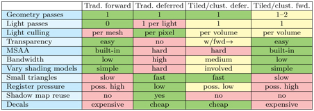
In summary, tiled, clustered, or other light-list culling techniques can be used with deferred or forward shading, and each can also be applied to decals. Algorithms for light-volume culling focus on minimizing the number of lights that are evaluated for each fragment, while the idea of decoupling geometry and shading can be used to balance processing and bandwidth costs to maximize efficiency. Just as frustum culling will cost additional time with no benefit if all objects are always in view, so will some techniques provide little benefit under various conditions. If the sun is the only light source, a light culling preprocess is not necessary. If there is little surface overdraw and few lights, deferred shading may cost more time overall. For scenes with many limited-effect sources of illumination, spending time to create localized light lists is worth the effort, whether using forward or deferred shading. When geometry is complex to process or surfaces are expensive to render, deferred shading provides a way to avoid overdraw, minimize driver costs such as program and state switches, and use fewer calls to render larger consolidated meshes. Keep in mind that several of these methods can be used in rendering a single frame. What makes for the best mix of techniques is not only dependent on the scene, but can also vary on a per-object or per-light basis [1589].

To conclude this section, we summarize the main differences among approaches in Table 20.1. The right arrow in the “Transparency” row means that deferred shading is applied to opaque surfaces, with forward shading needed for transparent ones. “Small triangles” notes an advantage of deferred shading, that quad shading (Section 23.1) can be inefficient when forward rendering, due to all four samples being fully evaluated. “Register pressure” refers to the overall complexity of the shaders involved. Using many registers in a shader can mean fewer threads formed, leading to the GPU’s warps being underused [134]. It can become low for tiled and clustered deferred techniques if shader streamlining methods are employed [273, 414, 1877]. Shadow map reuse is often not as critical as it once was, when GPU memory was more limited [1589].

Shadows are a challenge when a large number of light sources are present. One response is to ignore shadow computations for all but the closest and brightest lights, and the sun, at the risk of light leaks from the lesser sources. Harada et al. [667] discuss how they use ray casting in a tiled forward system, spawning a ray for each visible surface pixel to each nearby light source. Olsson et al. [1330, 1331] discuss generating shadow maps using occupied grid cells as proxies for geometry, with samples created as needed. They also present a hybrid system, combining these limited shadow maps with ray casting.

Using world space instead of screen space for generating light lists is another way to structure space for clustered shading. This approach can be reasonable in some situations, though might be worth avoiding for large scenes because of memory constraints [385] and because distant clusters will be pixel-sized, hurting performance. Persson [1386] provides code for a basic clustered forward system where static lights are stored in a three-dimensional world-space grid.

20.5 Deferred Texturing

Deferred shading avoids overdraw and its costs of computing a fragment’s shade and then having these results discarded. However, when forming G-buffers, overdraw still occurs. One object is rasterized and all its parameters are retrieved, performing several texture accesses along the way. If another object is drawn later that occludes these stored samples, all the bandwidth spent for rendering the first object was wasted. Some deferred shading systems perform a partial or full z-prepass to avoid texture access for a surface that is later drawn over by another object [38, 892, 1401]. However, an additional geometry pass is something many systems avoid if possible. Bandwidth is used by texture fetches, but also by vertex data access and other data. For detailed geometry, an extra pass can use more bandwidth than it might save in texture access costs.

The higher the number of G-buffers formed and accessed, the higher the memory and bandwidth costs. In some systems bandwidth may not be a concern, as the bottleneck could be predominantly within the GPU’s processor. As discussed at length in Chapter 18, there is always a bottleneck, and it can and will change from moment to moment. A major reason why there are so many efficiency schemes is that each is developed for a given platform and type of scene. Other factors, such as how hard it is to implement and optimize a system, the ease of authoring content, and a wide variety of other human factors, can also determine what is built.

While both computational and bandwidth capabilities of GPUs have risen over time, they have increased at different rates, with compute rising faster. This trend, combined with new functionality on the GPU, has meant that a way to future-proof your system is by aiming for the bottleneck to be GPU computation instead of buffer access [217, 1332].

A few different schemes have been developed that use a single geometry pass and avoid retrieving textures until needed. Haar and Aaltonen [625] describe how virtual deferred texturing is used in Assassin’s Creed Unity. Their system manages a local 8192 × 8192 texture atlas of visible textures, each with 128 × 128 resolution, selected from a much larger set. This atlas size permits storing (u, v) texture coordinates that can be used to access any texel in the atlas. There are 16 bits used to store a coordinate; with 13 bits needed for 8192 locations, this leaves 3 bits, i.e., 8 levels, for sub-texel precision. A 32-bit tangent basis is also stored, encoded as a quaternion [498] (Section 16.6). Doing so means only a single 64-bit G-buffer is needed. With no texture accesses performed in the geometry pass, overdraw can be extremely inexpensive. After this G-buffer is established, the virtual texture is then accessed during shading. Gradients are needed for mipmapping, but are not stored. Rather, each pixel’s neighbors are examined and those with the closest (u, v) values are used to compute the gradients on the fly. The material ID is also derived from determining which texture atlas tile is accessed, done by dividing the texture coordinate values by 128, i.e., the texture resolution.

Another technique used in this game to reduce shading costs is to render at a quarter resolution and use a special form of MSAA. On consoles using AMD GCN, or systems using OpenGL 4.5, OpenGL ES 3.2, or other extensions [2, 1406], the MSAA sampling pattern can be set as desired. Haar and Aaltonen set a grid pattern for 4× MSAA, so that each grid sample corresponds directly to the center of a full-screen pixel. By rendering at a quarter resolution, they can take advantage of the multisampling nature of MSAA. The (u, v) and tangent bases can be interpolated across the surface with no loss, and 8× MSAA (equivalent to 2× MSAA per pixel) is also possible. When rendering scenes with considerable overdraw, such as foliage and trees, their technique significantly reduces the number of shader invocations and bandwidth costs for the G-buffers.

Storing just the texture coordinates and basis is pretty minimal, but other schemes are possible. Burns and Hunt [217] describe what they call the visibility buffer, in which they store two pieces of data, a triangle ID and an instance ID. See Figure 20.12. The geometry pass shader is extremely quick, having no texture accesses and needing to store just these two ID values. All triangle and vertex data—positions, normals, color, material, and so on—are stored in global buffers. During the deferred shading pass, the triangle and instance IDs stored for each pixel are used to retrieve these data. The view ray for the pixel is intersected against the triangle to find the barycentric coordinates, which are used to interpolate among the triangle’s vertex data. Other computations that are normally done less frequently must also be performed per pixel, such as vertex shader calculations. Texture gradient values are also computed from scratch for each pixel, instead of being interpolated. All these data are then used to shade the pixel, applying lights using any classification scheme desired.

While this all sounds expensive, remember that computational power is growing faster than bandwidth capabilities. This research favors a compute-heavy pipeline that minimizes bandwidth losses due to overdraw. If there are less than 64k meshes in the scene, and each mesh has less than 64k triangles, each ID is then 16 bits in length and the G-buffer can be as small as 32 bits per pixel. Larger scenes push this to 48 or 64 bits.

Stachowiak [1685] describes a variant of the visibility buffer that uses some capabilities available on the GCN architecture. During the initial pass, the barycentric coordinates for the location on the triangle are also computed and stored per pixel. A GCN fragment (i.e., pixel) shader can compute the barycentric coordinates inexpensively, compared to later performing an individual ray/triangle intersection per pixel. While costing additional storage, this approach has an important advantage. With animated meshes the original visibility buffer scheme needs to have any modified mesh data streamed out to a buffer, so that the modified vertex locations can be retrieved during deferred shading. Saving the transformed mesh coordinates consumes additional bandwidth. By storing the barycentric coordinates in the first pass, we are done with the vertex positions, which do not have to be fetched again, a disadvantage of the original visibility buffer. However, if the distance from the camera is needed, this value must also be stored in the first pass, since it cannot later be reconstructed.

This pipeline lends itself to decoupling geometry and shading frequency, similar to previous schemes. Aaltonen [2] notes that the MSAA grid sampling method can be applied to each, leading to further reductions in the average amount of memory required. He also discusses variations in storage layout and differences in compute costs and capabilities for these three schemes. Schied and Dachsbacher [1561, 1562] go the other direction, building on the visibility buffer and using MSAA functionality to reduce memory consumption and shading computations for high-quality antialiasing. Pettineo [1407] notes that the availability of bindless texture functionality (Section 6.2.5) makes implementing deferred texturing simpler still. His deferred texturing system creates a larger G-buffer, storing the depth, a separate material ID, and depth gradients. Rendering the Sponza model, this system’s performance was compared against a clustered forward approach, with and without z-prepass. Deferred texturing was always faster than forward shading when MSAA was off, slowing when MSAA was applied. As noted in Section 5.4.2, most video games have moved away from MSAA as screen resolutions have increased, instead relying on temporal antialiasing, so in practical terms such support is not all that important.

Engel [433] notes that the visibility buffer concept has become more attractive due to API features exposed in DirectX 12 and Vulkan. Culling sets of triangles (Section 19.8) and other removal techniques performed using compute shaders reduce the number of triangles rasterized. DirectX 12’s ExecuteIndirect command can be used to create the equivalent of an optimized index buffer that displays only those triangles that were not culled. When used with an advanced culling system [1883, 1884], his analysis determined that the visibility buffer outperformed deferred shading at all resolutions and antialiasing settings on the San Miguel scene. As the screen resolution rose, the performance gap increased. Future changes to the GPU’s API and capabilities are likely to further improve performance. Lauritzen [993] discusses the visibility buffer and how there is a need to evolve the GPU to improve the way material shaders are accessed and processed in a deferred setting.

Doghramachi and Bucci [363] discuss their deferred texturing system in detail, which they call deferred+. Their system integrates aggressive culling techniques early on. For example, the previous frame’s depth buffer is downsampled and reprojected in a way that provides a conservative culling depth for each pixel in the current scene. These depths help test occlusion for rendering bounding volumes of all meshes visible in the frustum, as briefly discussed in Section 19.7.2. They note that the alpha cutout texture, if present, must be accessed in any initial pass (or any z-prepass, for that matter), so that objects behind cutouts are not hidden. The result of their culling and rasterization process is a set of G-buffers that include the depth, texture coordinates, tangent space, gradients, and material ID, which are used to shade the pixels. While its number of G-buffers is higher than in other deferred texturing schemes, it does avoid unneeded texture accesses. For two simplified scene models from Deus Ex: Mankind Divided, they found that deferred+ ran faster than clustered forward shading, and believe that more complex materials and lighting would further widen the gap. They also noted that warp usage was significantly better, meaning that tiny triangles caused fewer problems, so GPU tessellation performed better. Their implementation of deferred texturing has several other advantages over deferred shading, such as being able to handle a wider range of materials more efficiently. The main drawbacks are those common to most deferred schemes, relating to transparency and antialiasing.

20.6 Object- and Texture-Space Shading

The idea of decoupling the rate at which the geometry is sampled from the rate at which shading values are computed is a recurring theme in this chapter. Here we cover several alternate approaches that do not easily fit in the categories covered so far. In particular, we discuss hybrids that draw upon concepts first seen in the Reyes ¹ batch renderer [289], used for many years by Pixar and others to make their films. Now studios primarily use some form of ray or path tracing for rendering, but for its day, Reyes solved several rendering problems in an innovative and efficient way.

The key concept of Reyes is the idea of micropolygons. Every surface is diced into an extremely fine mesh of quadrilaterals. In the original system, dicing is done with respect to the eye, with the goal of having each micropolygon be about half the width and height of a pixel, so that the Nyquist limit (Section 5.4.1) is maintained. Quadrilaterals outside the frustum or facing away from the eye are culled. In this system, the micropolygon was shaded and assigned a single color. This technique evolved to shading the vertices in the micropolygon grid [63]. Our discussion here focuses on the original system, for the ideas it explored.

Each micropolygon is inserted into a jittered 4 × 4 sample grid in a pixel—a supersampled z-buffer. Jittering is done to avoid aliasing by producing noise instead. Because shading happens with respect to a micropolygon’s coverage, before rasterization, this type of technique is called object-based shading. Compare this to forward shading, where shading takes place in screen space during rasterization, and deferred shading, where it takes place after. See Figure 20.13.

One advantage of shading in object space is that material textures are often directly related to their micropolygons. That is, the geometric object can be subdivided such that there is a power-of-two number of texels in each micropolygon. During shading the exact filtered mipmap sample can then be retrieved for the micropolygon, since it directly correlates to the surface area shaded. The original Reyes system also meant that cache coherent access of a texture occurs, since micropolygons are accessed in order. This advantage does not hold for all textures, e.g., environment textures used as reflection maps must be sampled and filtered in traditional ways.

Motion blur and depth-of-field effects can also work well with this type of arrangement. For motion blur each micropolygon is assigned a position along its path at a jittered time during the frame interval. So, each micropolygon will have a different location along the direction of movement, giving a blur. Depth of field is achieved in a similar fashion, distributing the micropolygons based on the circle of confusion.

There are some disadvantages to the Reyes algorithm. All objects must be able to be tessellated, and must be diced to a fine degree. Shading occurs before occlusion testing in the z-buffer, so can be wasted due to overdraw. Sampling at the Nyquist limit does not mean that high-frequency phenomena such as sharp specular highlights are captured, but rather that sampling is sufficient to reconstruct lower frequencies.

Generally, every object must be “chartable,” in other words, must have (u, v) texture values for the vertices that give a unique texel for each different area on the model. See Figure 2.9 on page 23 and Figure 6.6 on page 173 for examples. Object-based shading can be thought of as first baking in the shading, with the camera used to determine view-dependent effects and possibly limit the amount of effort expended for each surface area. One simple method of performing object-based shading on the GPU is to tessellate the object to a fine subpixel level, then shade each vertex on the mesh. Doing so can be costly because the setup costs for each triangle are not amortized over a number of pixels. The expense is made worse still because a single-pixel triangle generates four pixel shader invocations, due to quad rendering (Section 23.1). GPUs are optimized to render triangles that cover a fair number of pixels, e.g., 16 or more (Section 23.10.3).

Burns et al. [216] explore object-space shading by performing it after establishing which object locations are visible. They determine these with a “polygon grid” for an object that is diced, culled as possible, and then rasterized. An independent object-space “shading grid” is then used to shade the visible areas, with each texel corresponding to an area of the surface. The shading grid can be a different resolution than the polygon grid. They found that a finely tessellated geometric surface provided little benefit, so decoupling the two led to more efficient use of the resources. They implemented their work only in a simulator, but their techniques have influenced newer research and development.

Considerable research that draws inspiration from Reyes has examined faster shading methods on the GPU for various phenomena. Ragan-Kelley et al. [1455] propose a hardware extension based on decoupled sampling, applying their idea to motion blur and depth of field. Samples have five dimensions: two for the subpixel location, two for the lens location, and one for time. Visibility and shading are sampled separately. A “decoupling mapping” determines the shading sample needed for a given visibility sample. Liktor and Dachsbacher [1042, 1043] present a deferred shading system in a similar vein, where shading samples are cached when computed and used during stochastic rasterization. Effects such as motion blur and depth of field do not require high sampling rates, so shading computations can be reused. Clarberg et al. [271] present hardware extensions for computing shading in texture space. These eliminate the quad overshading problem and hence allow for smaller triangles. Since shading is computed in texture space, the pixel shader can use a bilinear filter or a more complex one, when looking up the shading from the texture. This allows reducing shading costs by turning down the texture resolution. For low-frequency terms, this technique usually works well, since filtering can be used.

Andersson et al. [48] take a different approach, called texture-space shading. Each triangle is tested for frustum and backface culling, then its charted surface is applied to a corresponding area of an output target, shading this triangle based on its (u, v) parameterization. At the same time, using a geometry shader, each visible triangle’s size in the camera’s view is computed. This size value is used to determine in which mipmap-like level the triangle is inserted. In this way, the amount of shading performed for an object is related to its screen coverage. See Figure 20.14. They use stochastic rasterization to render the final image. Each fragment generated looks up its shaded color from the texture. Again, computed shading values can be reused for motion blur and depth-of-field effects.

Hillesland and Yang [747, 748] build upon the texture-space shading concept, along with caching concepts similar to Liktor and Dachsbacher’s. They draw geometry to the final view, use a compute shader to populate a mipmap-like structure of object-based shading results, and render the geometry again to access this texture and display the final shade. A triangle ID visibility buffer is also saved in the first pass, so that their compute shader can later access vertex attributes for interpolation. Their system includes coherence over time. Since the shading is in object space, the same area is associated with the same output texture location for each frame. If a surface area’s shade at a given mipmap level was computed previously and is not too old, it is reused instead of being recomputed. Results will vary with the material, lighting, and other factors, but they found that reusing a shading sample every other frame at 60 FPS led to negligible errors. They also determined that the mipmap level could be selected not only by screen size, but also by variation in other factors, such as the change in normal direction over an area. A higher mipmap level means that less shading is computed per screen fragment, which they found could lead to considerable savings.

Baker [94] describes Oxide Games’ renderer for the game Ashes of the Singularity. It is inspired by Reyes, though the implementation details are considerably different, and uses texture-space shading for each model as a whole. Objects may have any number of materials covering their surfaces, which are differentiated by using masks. Their process is:

• Several large—4k × 4k, 16 bits per channel—”master” textures are allocated for shading.
• All objects are evaluated. If in view, an object’s estimated area on the screen is computed.
• This area is used to assign a proportion of a master texture to each object. If the total requested area is larger than the texture space, proportions are scaled down to make the requests fit.
• Texture-based shading is performed in a compute shader, with each material attached to the model applied in turn. Results from each material are accumulated in the assigned master texture.
• Mipmap levels are computed for the master textures as needed.
• Objects are then rasterized, with the master textures used to shade them.

Using multiple materials per object allows such effects as having a single terrain model include dirt, roads, ground cover, water, snow, and ice, each with its own material BRDF. Antialiasing works on both a pixel level and a shader level, if desired, as the full information about an object’s surface area and its relationship to the master texture is accessible during shading. This ability allows the system to stably handle models with extremely high specular powers, for example. Because shaded results are attached to objects as a whole, regardless of visibility, shading can also be computed at a different frame rate than rasterization. Shading at 30 FPS was found to be adequate, with rasterization occurring at 60 FPS, or 90 FPS for virtual reality systems. Having asynchronous shading means that the frame rate for the geometry can be maintained even if the shader load becomes too high.

There are several challenges in implementing such a system. About twice as many batches are sent overall, compared to a typical game engine, since each object’s “material quadrilateral” is processed with a compute shader during the object-shading step, then the object is drawn during rasterization. Most batches are simple, however, and APIs such as DirectX 12 and Vulkan help remove overhead. How the master textures are allocated to objects based on their size makes a significant difference in image quality. Objects that are large on the screen, or otherwise vary in texel density, such as terrain, can have issues. Performing an additional stitching process is used to maintain a smooth transition among terrain tiles of different resolutions in the master texture. Screen-space techniques, such as ambient occlusion, are a challenge to implement. Like the original visibility buffer, animation affecting object shape must be done twice, for shading and for rasterization. Objects are shaded, then occluded, which is a source of waste. For an application with low depth complexity, such as a real-time strategy game, this cost can be relatively low. Each material is simple to evaluate, unlike complex deferred shaders, and shading is done on a chart for the whole object. Objects with simple shaders, such as particles and trees, receive little benefit from this technique. For performance, these effects can instead be rendered with forward shading. As can be seen in Figure 20.15, being able to handle many lights gives a richness to the rendered scene.

We end our discussion of efficient shading here. We have only touched upon a panoply of specialized techniques to improve speed and quality of results used in different applications. Our goal here is to present popular algorithms used to accelerate shading and explain how and why they arose. As graphics hardware capabilities and APIs evolve, and as screen resolutions, art workflows, and other elements change over time, efficient shading techniques will continue to be researched and developed in new and, likely, unanticipated ways.

If you have read the book through to this point, you now have working knowledge of the major algorithms that go into a modern interactive rendering engine. One of our goals is to get you up to speed so that you can comprehend current articles and presentations in the field. If you wish to see how these elements work together, we highly recommend you read the excellent articles on different commercial renderers by Courr`eges [293, 294] and Anagnostou [38]. After this point, the chapters that follow delve deeper into several fields, such as rendering for virtual and augmented reality, algorithms for intersection and collision detection, and architectural features of graphics hardware.

Further Reading and Resources

So, of the various mixes of these approaches—deferred, forward, tiled, clustered, visibility—which is better? Each has its own strengths, and the answer is “it depends.” Factors such as platform, scene characteristics, illumination model, and design goals can all play a part. As a starting spot, we recommend Pesce’s extensive discussions [1393, 1397] about the effectiveness and trade-offs of various schemes.

The SIGGRAPH course “Real-Time Many-Light Management and Shadows with Clustered Shading” [145, 1331, 1332, 1387] presents a thorough run-through of tiled and clustered shading techniques and their use with deferred and forward shading, along with related topics such as shadow mapping and implementing light classification on mobile devices. An earlier presentation by Stewart and Thomas [1700] explains tiled shading and presents copious timing results showing how various factors affect performance. Pettineo’s open-source framework [1401] compares tiled forward and deferred systems, and includes results for a wide range of GPUs.

For implementation details, the book on DirectX 11 by Zink et al. [1971] has about 50 pages on the subject of deferred shading and includes numerous code samples. The NVIDIA GameWorks code samples [1299] include an implementation of MSAA for deferred shading. The articles by Mikkelsen [1210] and O¨ rtegren and Persson [1340] in the book GPU Pro 7 describe modern GPU-based systems for tiled and clustered shading. Billeter et al. [144] give coding details on implementing tiled forward shading, and Stewart [1701] walks through code for performing tiled culling in a compute shader. Lauritzen [990] provides a full implementation for tiled deferred shading, and Pettineo [1401] builds a framework to compare it to tiled forward. Dufresne [390] has demo code for clustered forward shading. Persson [1386] provides code for a basic world-space clustered forward rendering solution. Finally, van Oosten [1334] discusses various optimizations and gives a demo system with code that implements different forms of clustered, tiled, and vanilla forward rendering, showing the performance differences.