
Chapter 6
Texturing
“All it takes is for the rendered image to look right.”
—Jim Blinn
A surface’s texture is its look and feel—just think of the texture of an oil painting. In computer graphics, texturing is a process that takes a surface and modifies its appearance at each location using some image, function, or other data source. As an example, instead of precisely representing the geometry of a brick wall, a color image of a brick wall is applied to a rectangle, consisting of two triangles. When the rectangle is viewed, the color image appears where the rectangle is located. Unless the viewer gets close to the wall, the lack of geometric detail will not be noticeable.
However, some textured brick walls can be unconvincing for reasons other than lack of geometry. For example, if the mortar is supposed to be matte, whereas the bricks are glossy, the viewer will notice that the roughness is the same for both materials. To produce a more convincing experience, a second image texture can be applied to the surface. Instead of changing the surface’s color, this texture changes the wall’s roughness, depending on location on the surface. Now the bricks and mortar have a color from the image texture and a roughness value from this new texture.
The viewer may see that now all the bricks are glossy and the mortar is not, but notice that each brick face appears to be perfectly flat. This does not look right, as bricks normally have some irregularity to their surfaces. By applying bump mapping, the shading normals of the bricks may be varied so that when they are rendered, they do not appear to be perfectly smooth. This sort of texture wobbles the direction of the rectangle’s original surface normal for purposes of computing lighting.
From a shallow viewing angle, this illusion of bumpiness can break down. The bricks should stick out above the mortar, obscuring it from view. Even from a straight-on view, the bricks should cast shadows onto the mortar. Parallax mapping uses a texture to appear to deform a flat surface when rendering it, and parallax occlusion mapping casts rays against a heightfield texture for improved realism. Displacement mapping truly displaces the surface by modifying triangle heights forming the model. Figure 6.1 shows an example with color texturing and bump mapping.

Figure 6.1. Texturing. Color and bump maps were applied to this fish to increase its visual level of detail. (Image courtesy of Elinor Quittner.)
These are examples of the types of problems that can be solved with textures, using more and more elaborate algorithms. In this chapter, texturing techniques are covered in detail. First, a general framework of the texturing process is presented. Next, we focus on using images to texture surfaces, since this is the most popular form of texturing used in real-time work. Procedural textures are briefly discussed, and then some common methods of having textures affect the surface are explained.
6.1 The Texturing Pipeline
Texturing is a technique for efficiently modeling variations in a surface’s material and finish. One way to think about texturing is to consider what happens for a single shaded pixel. As seen in the previous chapter, the shade is computed by taking into account the color of the material and the lights, among other factors. If present, transparency also affects the sample. Texturing works by modifying the values used in the shading equation. The way these values are changed is normally based on the position on the surface. So, for the brick wall example, the color at any point on the surface is replaced by a corresponding color in the image of a brick wall, based on the surface location. The pixels in the image texture are often called texels, to differentiate them from the pixels on the screen. The roughness texture modifies the roughness value, and the bump texture changes the direction of the shading normal, so each of these change the result of the shading equation.
Texturing can be described by a generalized texture pipeline. Much terminology will be introduced in a moment, but take heart: Each piece of the pipeline will be described in detail.
A location in space is the starting point for the texturing process. This location can be in world space, but is more often in the model’s frame of reference, so that as the model moves, the texture moves along with it. Using Kershaw’s terminology [884], this point in space then has a projector function applied to it to obtain a set of numbers, called texture coordinates, that will be used for accessing the texture. This process is called mapping, which leads to the phrase texture mapping. Sometimes the texture image itself is called the texture map, though this is not strictly correct.
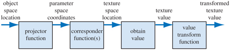
Figure 6.2. The generalized texture pipeline for a single texture.
Before these new values may be used to access the texture, one or more corresponder functions can be used to transform the texture coordinates to texture space. These texture-space locations are used to obtain values from the texture, e.g., they may be array indices into an image texture to retrieve a pixel. The retrieved values are then potentially transformed yet again by a value transform function, and finally these new values are used to modify some property of the surface, such as the material or shading normal. Figure 6.2 shows this process in detail for the application of a single texture. The reason for the complexity of the pipeline is that each step provides the user with a useful control. It should be noted that not all steps need to be activated at all times.

Figure 6.3. Pipeline for a brick wall.
Using this pipeline, this is what happens when a triangle has a brick wall texture and a sample is generated on its surface (see Figure 6.3). The (x, y, z) position in the object’s local frame of reference is found; say it is . A projector function is then applied to this position. Just as a map of the world is a projection of a three-dimensional object into two dimensions, the projector function here typically changes the (x, y, z) vector into a two-element vector (u, v). The projector function used for this example is equivalent to an orthographic projection (Section 2.3.1), acting something like a slide projector shining the brick wall image onto the triangle’s surface. To return to the wall, a point on its surface could be transformed into a pair of values ranging from 0 to 1. Say the values obtained are (0.32, 0.29). These texture coordinates are to be used to find what the color of the image is at this location. The resolution of our brick texture is, say, , so the corresponder function multiplies the (u, v) by 256 each, giving (81.92, 74.24). Dropping the fractions, pixel (81, 74) is found in the brick wall image, and is of color (0.9, 0.8, 0.7). The texture color is in sRGB color space, so if the color is to be used in shading equations, it is converted to linear space, giving (0.787, 0.604, 0.448) (Section 5.6).
6.1.1. The Projector Function
The first step in the texture process is obtaining the surface’s location and projecting it into texture coordinate space, usually two-dimensional (u, v) space. Modeling packages typically allow artists to define (u, v)-coordinates per vertex. These may be initialized from projector functions or from mesh unwrapping algorithms. Artists can edit (u, v)-coordinates in the same way they edit vertex positions. Projector functions typically work by converting a three-dimensional point in space into texture coordinates. Functions commonly used in modeling programs include spherical, cylindrical, and planar projections [141,884,970].
Other inputs can be used to a projector function. For example, the surface normal can be used to choose which of six planar projection directions is used for the surface. Problems in matching textures occur at the seams where the faces meet; Geiss [521,522] discusses a technique of blending among them. Tarini et al. [1740] describe polycube maps, where a model is mapped to a set of cube projections, with different volumes of space mapping to different cubes.
Other projector functions are not projections at all, but are an implicit part of surface creation and tessellation. For example, parametric curved surfaces have a natural set of (u, v) values as part of their definition. See Figure 6.4. The texture coordinates could also be generated from all sorts of different parameters, such as the view direction, temperature of the surface, or anything else imaginable. The goal of the projector function is to generate texture coordinates. Deriving these as a function of position is just one way to do it.

Figure 6.4. Different texture projections. Spherical, cylindrical, planar, and natural (u, v) projections are shown, left to right. The bottom row shows each of these projections applied to a single object (which has no natural projection).

Figure 6.5. How various texture projections are used on a single model. Box mapping consists of six planar mappings, one for each box face. (Images courtesy of Tito Pagán.)
Non-interactive renderers often call these projector functions as part of the rendering process itself. A single projector function may suffice for the whole model, but often the artist has to use tools to subdivide the model and apply various projector functions separately [1345]. See Figure 6.5.
In real-time work, projector functions are usually applied at the modeling stage, and the results of the projection are stored at the vertices. This is not always the case; sometimes it is advantageous to apply the projection function in the vertex or pixel shader. Doing so can increase precision, and helps enable various effects, including animation (Section 6.4). Some rendering methods, such as environment mapping (Section 10.4), have specialized projector functions of their own that are evaluated per pixel.
The spherical projection (on the left in Figure 6.4) casts points onto an imaginary sphere centered around some point. This projection is the same as used in Blinn and Newell’s environment mapping scheme (Section 10.4.1), so Equation on page 407 describes this function. This projection method suffers from the same problems of vertex interpolation described in that section.
Cylindrical projection computes the u texture coordinate the same as spherical projection, with the v texture coordinate computed as the distance along the cylinder’s axis. This projection is useful for objects that have a natural axis, such as surfaces of revolution. Distortion occurs when surfaces are near-perpendicular to the cylinder’s axis.
The planar projection is like an x-ray beam, projecting in parallel along a direction and applying the texture to all surfaces. It uses orthographic projection (Section 4.7.1). This type of projection is useful for applying decals, for example (Section 20.2).
As there is severe distortion for surfaces that are edge-on to the projection direction, the artist often must manually decompose the model into near-planar pieces. There are also tools that help minimize distortion by unwrapping the mesh, or creating a near-optimal set of planar projections, or that otherwise aid this process. The goal is to have each polygon be given a fairer share of a texture’s area, while also maintaining as much mesh connectivity as possible. Connectivity is important in that sampling artifacts can appear along edges where separate parts of a texture meet. A mesh with a good unwrapping also eases the artist’s work [970,1345]. Section 16.2.1 discusses how texture distortion can adversely affect rendering. Figure 6.6 shows the workspace used to create the statue in Figure 6.5. This unwrapping process is one facet of a larger field of study, mesh parameterization. The interested reader is referred to the SIGGRAPH course notes by Hormann et al. [774].

Figure 6.6. Several smaller textures for the statue model, saved in two larger textures. The right figure shows how the triangle mesh is unwrapped and displayed on the texture to aid in its creation. (Images courtesy of Tito Pagán.)
The texture coordinate space is not always a two-dimensional plane; sometimes it is a three-dimensional volume. In this case, the texture coordinates are presented as a three-element vector, (u, v, w), with w being depth along the projection direction. Other systems use up to four coordinates, often designated (s, t, r, q) [885]; q is used as the fourth value in a homogeneous coordinate. It acts like a movie or slide projector, with the size of the projected texture increasing with distance. As an example, it is useful for projecting a decorative spotlight pattern, called a gobo, onto a stage or other surface [1597].
Another important type of texture coordinate space is directional, where each point in the space is accessed by an input direction. One way to visualize such a space is as points on a unit sphere, the normal at each point representing the direction used to access the texture at that location. The most common type of texture using a directional parameterization is the cube map (Section 6.2.4).
It is also worth noting that one-dimensional texture images and functions have their uses. For example, on a terrain model the coloration can be determined by altitude, e.g., the lowlands are green; the mountain peaks are white. Lines can also be textured; one use of this is to render rain as a set of long lines textured with a semitransparent image. Such textures are also useful for converting from one value to another, i.e., as a lookup table.
Since multiple textures can be applied to a surface, multiple sets of texture coordinates may need to be defined. However the coordinate values are applied, the idea is the same: These texture coordinates are interpolated across the surface and used to retrieve texture values. Before being interpolated, however, these texture coordinates are transformed by corresponder functions.
6.1.2. The Corresponder Function
Corresponder functions convert texture coordinates to texture-space locations. They provide flexibility in applying textures to surfaces. One example of a corresponder function is to use the API to select a portion of an existing texture for display; only this subimage will be used in subsequent operations.
Another type of corresponder is a matrix transformation, which can be applied in the vertex or pixel shader. This enables to translating, rotating, scaling, shearing, or projecting the texture on the surface. As discussed in Section 4.1.5, the order of transforms matters. Surprisingly, the order of transforms for textures must be the reverse of the order one would expect. This is because texture transforms actually affect the space that determines where the image is seen. The image itself is not an object being transformed; the space defining the image’s location is being changed.
Another class of corresponder functions controls the way an image is applied. We know that an image will appear on the surface where (u, v) are in the [0, 1] range. But what happens outside of this range? Corresponder functions determine the behavior. In OpenGL, this type of corresponder function is called the “wrapping mode”; in DirectX, it is called the “texture addressing mode.” Common corresponder functions of this type are:
- wrap (DirectX), repeat (OpenGL), or tile—The image repeats itself across the surface; algorithmically, the integer part of the texture coordinates is dropped. This function is useful for having an image of a material repeatedly cover a surface, and is often the default.
- mirror—The image repeats itself across the surface, but is mirrored (flipped) on every other repetition. For example, the image appears normally going from 0 to 1, then is reversed between 1 and 2, then is normal between 2 and 3, then is reversed, and so on. This provides some continuity along the edges of the texture.
- clamp (DirectX) or clamp to edge (OpenGL)—Values outside the range [0, 1] are clamped to this range. This results in the repetition of the edges of the image texture. This function is useful for avoiding accidentally taking samples from the opposite edge of a texture when bilinear interpolation happens near a texture’s edge [885].
- border (DirectX) or clamp to border (OpenGL)—Texture coordinates outside [0, 1] are rendered with a separately defined border color. This function can be good for rendering decals onto single-color surfaces, for example, as the edge of the texture will blend smoothly with the border color.
See Figure 6.7. These corresponder functions can be assigned differently for each texture axis, e.g., the texture could repeat along the u-axis and be clamped on the v-axis. In DirectX there is also a mirror once mode that mirrors a texture once along the zero value for the texture coordinate, then clamps, which is useful for symmetric decals.

Figure 6.7. Image texture repeat, mirror, clamp, and border functions in action.
Repeated tiling of a texture is an inexpensive way of adding more visual detail to a scene. However, this technique often looks unconvincing after about three repetitions of the texture, as the eye picks out the pattern. A common solution to avoid such periodicity problems is to combine the texture values with another, non-tiled, texture. This approach can be considerably extended, as seen in the commercial terrain rendering system described by Andersson [40]. In this system, multiple textures are combined based on terrain type, altitude, slope, and other factors. Texture images are also tied to where geometric models, such as bushes and rocks, are placed within the scene.
Another option to avoid periodicity is to use shader programs to implement specialized corresponder functions that randomly recombine texture patterns or tiles. Wang tiles are one example of this approach. A Wang tile set is a small set of square tiles with matching edges. Tiles are selected randomly during the texturing process [1860]. Lefebvre and Neyret [1016] implement a similar type of corresponder function using dependent texture reads and tables to avoid pattern repetition.
The last corresponder function applied is implicit, and is derived from the image’s size. A texture is normally applied within the range [0, 1] for u and v. As shown in the brick wall example, by multiplying texture coordinates in this range by the resolution of the image, one may obtain the pixel location. The advantage of being able to specify (u, v) values in a range of [0, 1] is that image textures with different resolutions can be swapped in without having to change the values stored at the vertices of the model.
6.1.3. Texture Values
After the corresponder functions are used to produce texture-space coordinates, the coordinates are used to obtain texture values. For image textures, this is done by accessing the texture to retrieve texel information from the image. This process is dealt with extensively in Section 6.2. Image texturing constitutes the vast majority of texture use in real-time work, but procedural functions can also be used. In the case of procedural texturing, the process of obtaining a texture value from a texture-space location does not involve a memory lookup, but rather the computation of a function. Procedural texturing is further described in Section 6.3f.
The most straightforward texture value is an RGB triplet that is used to replace or modify the surface colors; similarly, a single grayscale value could be returned. Another type of data to return is RGB , as described in Section 5.5. The (alpha) value is normally the opacity of the color, which determines the extent to which the color may affect the pixel. That said, any other value could be stored, such as surface roughness. There are many other types of data that can be stored in image textures, as will be seen when bump mapping is discussed in detail (Section 6.7).
The values returned from the texture are optionally transformed before use. These transformations may be performed in the shader program. One common example is the remapping of data from an unsigned range (0.0 to 1.0) to a signed range ( to 1.0), which is used for shading normals stored in a color texture.
6.2 Image Texturing
In image texturing, a two-dimensional image is effectively glued onto the surface of one or more triangles. We have walked through the process of computing a texture-space location; now we will address the issues and algorithms for obtaining a texture value from the image texture, given that location. For the rest of this chapter, the image texture will be referred to simply as the texture. In addition, when we refer to a pixel’s cell here, we mean the screen grid cell surrounding that pixel. As discussed in Section 5.4.1, a pixel is actually a displayed color value that can (and should, for better quality) be affected by samples outside of its associated grid cell.
In this section we particularly focus on methods to rapidly sample and filter textured images. Section 5.4.2 discussed the problem of aliasing, especially with respect to rendering edges of objects. Textures can also have sampling problems, but they occur within the interiors of the triangles being rendered.
The pixel shader accesses textures by passing in texture coordinate values to a call such as texture2D. These values are in (u, v) texture coordinates, mapped by a corresponder function to a range [0.0, 1.0]. The GPU takes care of converting this value to texel coordinates. There are two main differences among texture coordinate systems in different APIs. In DirectX the upper left corner of the texture is (0, 0) and the lower right is (1, 1). This matches how many image types store their data, the top row being the first one in the file. In OpenGL the texel (0, 0) is located in the lower left, a y-axis flip from DirectX. Texels have integer coordinates, but we often want to access a location between texels and blend among them. This brings up the question of what the floating point coordinates of the center of a pixel are. Heckbert [692] discusses how there are two systems possible: truncating and rounding. DirectX 9 defined each center at (0.0, 0.0)—this uses rounding. This system was somewhat confusing, as the upper left corner of the upper left pixel, at DirectX’s origin, then had the value . DirectX 10 onward changes to OpenGL’s system, where the center of a texel has the fractional values (0.5, 0.5)—truncation, or more accurately, flooring, where the fraction is dropped. Flooring is a more natural system that maps well to language, in that pixel (5, 9), for example, defines a range from 5.0 to 6.0 for the u-coordinate and 9.0 to 10.0 for the v.
One term worth explaining at this point is dependent texture read, which has two definitions. The first applies to mobile devices in particular. When accessing a texture via texture2D or similar, a dependent texture read occurs whenever the pixel shader calculates texture coordinates instead of using the unmodified texture coordinates passed in from the vertex shader [66]. Note that this means any change at all to the incoming texture coordinates, even such simple actions as swapping the u and v values. Older mobile GPUs, those that do not support OpenGL ES 3.0, run more efficiently when the shader has no dependent texture reads, as the texel data can then be prefetched. The other, older, definition of this term was particularly important for early desktop GPUs. In this context a dependent texture read occurs when one texture’s coordinates are dependent on the result of some previous texture’s values. For example, one texture might change the shading normal, which in turn changes the coordinates used to access a cube map. Such functionality was limited or even non-existent on early GPUs. Today such reads can have an impact on performance, depending on the number of pixels being computed in a batch, among other factors. See Section 23.8 for more information.
The texture image size used in GPUs is usually texels, where m and n are non-negative integers. These are referred to as power-of-two (POT) textures. Modern GPUs can handle non-power-of-two (NPOT) textures of arbitrary size, which allows a generated image to be treated as a texture. However, some older mobile GPUs may not support mipmapping (Section 6.2.2) for NPOT textures. Graphics accelerators have different upper limits on texture size. DirectX 12 allows a maximum of texels, for example.
Assume that we have a texture of size texels and that we want to use it as a texture on a square. As long as the projected square on the screen is roughly the same size as the texture, the texture on the square looks almost like the original image. But what happens if the projected square covers ten times as many pixels as the original image contains (called magnification), or if the projected square covers only a small part of the screen (minification)? The answer is that it depends on what kind of sampling and filtering methods you decide to use for these two separate cases.
The image sampling and filtering methods discussed in this chapter are applied to the values read from each texture. However, the desired result is to prevent aliasing in the final rendered image, which in theory requires sampling and filtering the final pixel colors. The distinction here is between filtering the inputs to the shading equation, or filtering its output. As long as the inputs and output are linearly related (which is true for inputs such as colors), then filtering the individual texture values is equivalent to filtering the final colors. However, many shader input values stored in textures, such as surface normals and roughness values, have a nonlinear relationship to the output. Standard texture filtering methods may not work well for these textures, resulting in aliasing. Improved methods for filtering such textures are discussed in Section 9.13.
6.2.1. Magnification
In Figure 6.8, a texture of size texels is textured onto a square, and the square is viewed rather closely with respect to the texture size, so the underlying graphics system has to magnify the texture. The most common filtering techniques for magnification are nearest neighbor (the actual filter is called a box filter—see Section 5.4.1) and bilinear interpolation. There is also cubic convolution, which uses the weighted sum of a or array of texels. This enables much higher magnification quality. Although native hardware support for cubic convolution (also called bicubic interpolation) is currently not commonly available, it can be performed in a shader program.

Figure 6.8. Texture magnification of a image onto pixels. Left: nearest neighbor filtering, where the nearest texel is chosen per pixel. Middle: bilinear filtering using a weighted average of the four nearest texels. Right: cubic filtering using a weighted average of the nearest texels.
In the left part of Figure 6.8, the nearest neighbor method is used. One characteristic of this magnification technique is that the individual texels may become apparent. This effect is called pixelation and occurs because the method takes the value of the nearest texel to each pixel center when magnifying, resulting in a blocky appearance. While the quality of this method is sometimes poor, it requires only one texel to be fetched per pixel.
In the middle image of the same figure, bilinear interpolation (sometimes called linear interpolation) is used. For each pixel, this kind of filtering finds the four neighboring texels and linearly interpolates in two dimensions to find a blended value for the pixel. The result is blurrier, and much of the jaggedness from using the nearest neighbor method has disappeared. As an experiment, try looking at the left image while squinting, as this has approximately the same effect as a low-pass filter and reveals the face a bit more.
Returning to the brick texture example on page : Without dropping the fractions, we obtained . We use OpenGL’s lower left origin texel coordinate system here, since it matches the standard Cartesian system. Our goal is to interpolate among the four closest texels, defining a texel-sized coordinate system using their texel centers. See Figure 6.9.

Figure 6.9. Bilinear interpolation. The four texels involved are illustrated by the four squares on the left, texel centers in blue. On the right is the coordinate system formed by the centers of the four texels.
To find the four nearest pixels, we subtract the pixel center fraction (0.5, 0.5) from our sample location, giving (81.42, 73.74). Dropping the fractions, the four closest pixels range from to . The fractional part, (0.42, 0.74) for our example, is the location of the sample relative to the coordinate system formed by the four texel centers. We denote this location as .
Define the texture access function as , where x and y are integers and the color of the texel is returned. The bilinearly interpolated color for any location can be computed as a two-step process. First, the bottom texels, and , are interpolated horizontally (using ), and similarly for the topmost two texels, and . For the bottom texels, we obtain (bottom green circle in Figure 6.9), and for the top, (top green circle). These two values are then interpolated vertically (using ), so the bilinearly interpolated color at is
(6.1)
Intuitively, a texel closer to our sample location will influence its final value more. This is indeed what we see in this equation. The upper right texel at has an influence of . Note the symmetry: The upper right’s influence is equal to the area of the rectangle formed by the lower left corner and the sample point. Returning to our example, this means that the value retrieved from this texel will be multiplied by , specifically 0.3108. Clockwise from this texel the other multipliers are , , and , all four of these weights summing to 1.0.
A common solution to the blurriness that accompanies magnification is to use detail textures. These are textures that represent fine surface details, from scratches on a cellphone to bushes on terrain. Such detail is overlaid onto the magnified texture as a separate texture, at a different scale. The high-frequency repetitive pattern of the detail texture, combined with the low-frequency magnified texture, has a visual effect similar to the use of a single high-resolution texture.
Bilinear interpolation interpolates linearly in two directions. However, a linear interpolation is not required. Say a texture consists of black and white pixels in a checkerboard pattern. Using bilinear interpolation gives varying grayscale samples across the texture. By remapping so that, say, all grays lower than 0.4 are black, all grays higher than 0.6 are white, and those in between are stretched to fill the gap, the texture looks more like a checkerboard again, while also giving some blend between texels. See Figure 6.10.

Figure 6.10. Nearest neighbor, bilinear interpolation, and part way in between by remapping, using the same checkerboard texture. Note how nearest neighbor sampling gives slightly different square sizes, since the texture and the image grid do not match perfectly.
Using a higher-resolution texture would have a similar effect. For example, imagine each checker square consists of texels instead of being . Around the center of each checker, the interpolated color would be fully black or white.
To the right in Figure 6.8, a bicubic filter has been used, and the remaining blockiness is largely removed. It should be noted that bicubic filters are more expensive than bilinear filters. However, many higher-order filters can be expressed as repeated linear interpolations [1518] (see also Section 17.1.1). As a result, the GPU hardware for linear interpolation in the texture unit can be exploited with several lookups.
If bicubic filters are considered too expensive, Quílez [1451] proposes a simple technique using a smooth curve to interpolate in between a set of texels. We first describe the curves and then the technique. Two commonly used curves are the smoothstep curve and the quintic curve [1372]:
(6.2)
These are useful for many other situations where you want to smoothly interpolate from one value to another. The smoothstep curve has the property that , and it is smooth between 0 and 1. The quintic curve has the same properties, but also , i.e., the second derivatives are also 0 at the start and end of the curve. The two curves are shown in Figure 6.11.

Figure 6.11. The smoothstep curve s(x) (left) and a quintic curve q(x) (right).

Figure 6.12. Four different ways to magnify a one-dimensional texture. The orange circles indicate the centers of the texels as well as the texel values (height). From left to right: nearest neighbor, linear, using a quintic curve between each pair of neighboring texels, and using cubic interpolation.
The technique starts by computing (same as used in Equation 6.1 and in Figure 6.9) by first multiplying the sample by the texture dimensions and adding 0.5. The integer parts are kept for later, and the fractions are stored in and , which are in the range of [0, 1]. The are then transformed as , still in the range of [0, 1]. Finally, 0.5 is subtracted and the integer parts are added back in; the resulting u-coordinate is then divided by the texture width, and similarly for v. At this point, the new texture coordinates are used with the bilinear interpolation lookup provided by the GPU. Note that this method will give plateaus at each texel, which means that if the texels are located on a plane in RGB space, for example, then this type of interpolation will give a smooth, but still staircased, look, which may not always be desired. See Figure 6.12.
6.2.2. Minification
When a texture is minimized, several texels may cover a pixel’s cell, as shown in Figure 6.13. To get a correct color value for each pixel, you should integrate the effect of the texels influencing the pixel. However, it is difficult to determine precisely the exact influence of all texels near a particular pixel, and it is effectively impossible to do so perfectly in real time.
Because of this limitation, several different methods are used on GPUs. One method is to use the nearest neighbor, which works exactly as the corresponding magnification filter does, i.e., it selects the texel that is visible at the center of the pixel’s cell. This filter may cause severe aliasing problems. In Figure 6.14, nearest neighbor is used in the top figure. Toward the horizon, artifacts appear because only one of the many texels influencing a pixel is chosen to represent the surface. Such artifacts are even more noticeable as the surface moves with respect to the viewer, and are one manifestation of what is called temporal aliasing.
Another filter often available is bilinear interpolation, again working exactly as in the magnification filter. This filter is only slightly better than the nearest neighbor approach for minification. It blends four texels instead of using just one, but when a pixel is influenced by more than four texels, the filter soon fails and produces aliasing.
Better solutions are possible. As discussed in Section 5.4.1, the problem of aliasing can be addressed by sampling and filtering techniques. The signal frequency of a texture depends upon how closely spaced its texels are on the screen. Due to the Nyquist limit, we need to make sure that the texture’s signal frequency is no greater than half the sample frequency. For example, say an image is composed of alternating black and white lines, a texel apart. The wavelength is then two texels wide (from black line to black line), so the frequency is . To properly display this texture on a screen, the frequency must then be at least , i.e., at least one pixel per texel. So, for textures in general, there should be at most one texel per pixel to avoid aliasing.

Figure 6.13. Minification: A view of a checkerboard-textured square through a row of pixel cells, showing roughly how a number of texels affect each pixel.

Figure 6.14. The top image was rendered with point sampling (nearest neighbor), the center with mipmapping, and the bottom with summed area tables.
To achieve this goal, either the pixel’s sampling frequency has to increase or the texture frequency has to decrease. The antialiasing methods discussed in the previous chapter give ways to increase the pixel sampling rate. However, these give only a limited increase in sampling frequency. To more fully address this problem, various texture minification algorithms have been developed.
The basic idea behind all texture antialiasing algorithms is the same: to preprocess the texture and create data structures that will help compute a quick approximation of the effect of a set of texels on a pixel. For real-time work, these algorithms have the characteristic of using a fixed amount of time and resources for execution. In this way, a fixed number of samples are taken per pixel and combined to compute the effect of a (potentially huge) number of texels.
Mipmapping
The most popular method of antialiasing for textures is called mipmapping [1889]. It is implemented in some form on all graphics accelerators now produced. “Mip” stands for multum in parvo, Latin for “many things in a small place”—a good name for a process in which the original texture is filtered down repeatedly into smaller images.

Figure 6.15. A mipmap is formed by taking the original image (level 0), at the base of the pyramid, and averaging each area into a texel value on the next level up. The vertical axis is the third texture coordinate, d. In this figure, d is not linear; it is a measure of which two texture levels a sample uses for interpolation.
When the mipmapping minimization filter is used, the original texture is augmented with a set of smaller versions of the texture before the actual rendering takes place. The texture (at level zero) is downsampled to a quarter of the original area, with each new texel value often computed as the average of four neighbor texels in the original texture. The new, level-one texture is sometimes called a subtexture of the original texture. The reduction is performed recursively until one or both of the dimensions of the texture equals one texel. This process is illustrated in Figure 6.15. The set of images as a whole is often called a mipmap chain.
Two important elements in forming high-quality mipmaps are good filtering and gamma correction. The common way to form a mipmap level is to take each set of texels and average them to get the mip texel value. The filter used is then a box filter, one of the worst filters possible. This can result in poor quality, as it has the effect of blurring low frequencies unnecessarily, while keeping some high frequencies that cause aliasing [172]. It is better to use a Gaussian, Lanczos, Kaiser, or similar filter; fast, free source code exists for the task [172,1592], and some APIs support better filtering on the GPU itself. Near the edges of textures, care must be taken during filtering as to whether the texture repeats or is a single copy.
For textures encoded in a nonlinear space (such as most color textures), ignoring gamma correction when filtering will modify the perceived brightness of the mipmap levels [173,607]. As you get farther away from the object and the uncorrected mipmaps get used, the object can look darker overall, and contrast and details can also be affected. For this reason, it is important to convert such textures from sRGB to linear space (Section 5.6), perform all mipmap filtering in that space, and convert the final results back into sRGB color space for storage. Most APIs have support for sRGB textures, and so will generate mipmaps correctly in linear space and store the results in sRGB. When sRGB textures are accessed, their values are first converted to linear space so that magnification and minification are performed properly.
As mentioned earlier, some textures have a fundamentally nonlinear relationship to the final shaded color. Although this poses a problem for filtering in general, mipmap generation is particularly sensitive to this issue, since many hundred or thousands of pixels are being filtered. Specialized mipmap generation methods are often needed for the best results. Such methods are detailed in Section 9.13.
The basic process of accessing this structure while texturing is straightforward. A screen pixel encloses an area on the texture itself. When the pixel’s area is projected onto the texture (Figure 6.16), it includes one or more texels. Using the pixel’s cell boundaries is not strictly correct, but is used here to simplify the presentation. Texels outside of the cell can influence the pixel’s color; see Section 5.4.1. The goal is to determine roughly how much of the texture influences the pixel. There are two common measures used to compute d (which OpenGL calls , and which is also known as the texture level of detail). One is to use the longer edge of the quadrilateral formed by the pixel’s cell to approximate the pixel’s coverage [1889]; another is to use as a measure the largest absolute value of the four differentials , , , and [901,1411]. Each differential is a measure of the amount of change in the texture coordinate with respect to a screen axis. For example, is the amount of change in the u texture value along the x-screen-axis for one pixel. See Williams’s original article [1889] or the articles by Flavell [473] or Pharr [1411] for more about these equations. McCormack et al. [1160] discuss the introduction of aliasing by the largest absolute value method, and they present an alternate formula. Ewins et al. [454] analyze the hardware costs of several algorithms of comparable quality.

Figure 6.16. On the left is a square pixel cell and its view of a texture. On the right is the projection of the pixel cell onto the texture itself.
These gradient values are available to pixel shader programs using Shader Model 3.0 or newer. Since they are based on the differences between values in adjacent pixels, they are not accessible in sections of the pixel shader affected by dynamic flow control (Section 3.8). For texture reads to be performed in such a section (e.g., inside a loop), the derivatives must be computed earlier. Note that since vertex shaders cannot access gradient information, the gradients or the level of detail need to be computed in the vertex shader itself and supplied to the GPU when using vertex texturing.
The intent of computing the coordinate d is to determine where to sample along the mipmap’s pyramid axis. See Figure 6.15. The goal is a pixel-to-texel ratio of at least 1 : 1 to achieve the Nyquist rate. The important principle here is that as the pixel cell comes to include more texels and d increases, a smaller, blurrier version of the texture is accessed. The (u, v, d) triplet is used to access the mipmap. The value d is analogous to a texture level, but instead of an integer value, d has the fractional value of the distance between levels. The texture level above and the level below the d location is sampled. The (u, v) location is used to retrieve a bilinearly interpolated sample from each of these two texture levels. The resulting sample is then linearly interpolated, depending on the distance from each texture level to d. This entire process is called trilinear interpolation and is performed per pixel.
One user control on the d-coordinate is the level of detail bias (LOD bias). This is a value added to d, and so it affects the relative perceived sharpness of a texture. If we move further up the pyramid to start (increasing d), the texture will look blurrier. A good LOD bias for any given texture will vary with the image type and with the way it is used. For example, images that are somewhat blurry to begin with could use a negative bias, while poorly filtered (aliased) synthetic images used for texturing could use a positive bias. The bias can be specified for the texture as a whole, or per-pixel in the pixel shader. For finer control, the d-coordinate or the derivatives used to compute it can be supplied by the user.
The benefit of mipmapping is that, instead of trying to sum all the texels that affect a pixel individually, precombined sets of texels are accessed and interpolated. This process takes a fixed amount of time, no matter what the amount of minification. However, mipmapping has several flaws [473]. A major one is overblurring. Imagine a pixel cell that covers a large number of texels in the u-direction and only a few in the v-direction. This case commonly occurs when a viewer looks along a textured surface nearly edge-on. In fact, it is possible to need minification along one axis of the texture and magnification along the other. The effect of accessing the mipmap is that square areas on the texture are retrieved; retrieving rectangular areas is not possible. To avoid aliasing, we choose the largest measure of the approximate coverage of the pixel cell on the texture. This results in the retrieved sample often being relatively blurry. This effect can be seen in the mipmap image in Figure 6.14. The lines moving into the distance on the right show overblurring.

Figure 6.17. The pixel cell is back-projected onto the texture, bound by a rectangle; the four corners of the rectangle are used to access the summed-area table.
Summed-Area Table
Another method to avoid overblurring is the summed-area table (SAT) [312]. To use this method, one first creates an array that is the size of the texture but contains more bits of precision for the color stored (e.g., 16 bits or more for each of red, green, and blue). At each location in this array, one must compute and store the sum of all the corresponding texture’s texels in the rectangle formed by this location and texel (0, 0) (the origin). During texturing, the pixel cell’s projection onto the texture is bound by a rectangle. The summed-area table is then accessed to determine the average color of this rectangle, which is passed back as the texture’s color for the pixel. The average is computed using the texture coordinates of the rectangle shown in Figure 6.17. This is done using the formula given in Equation 6.3:
(6.3)
Here, x and y are the texel coordinates of the rectangle and is the summed-area value for that texel. This equation works by taking the sum of the entire area from the upper right corner to the origin, then subtracting off areas A and B by subtracting the neighboring corners’ contributions. Area C has been subtracted twice, so it is added back in by the lower left corner. Note that is the upper right corner of area C, i.e., is the lower left corner of the bounding box.
The results of using a summed-area table are shown in Figure 6.14. The lines going to the horizon are sharper near the right edge, but the diagonally crossing lines in the middle are still overblurred. The problem is that when a texture is viewed along its diagonal, a large rectangle is generated, with many of the texels situated nowhere near the pixel being computed. For example, imagine a long, thin rectangle representing the pixel cell’s back-projection lying diagonally across the entire texture in Figure 6.17. The whole texture rectangle’s average will be returned, rather than just the average within the pixel cell.
The summed-area table is an example of what are called anisotropic filtering algorithms [691]. Such algorithms retrieve texel values over areas that are not square. However, SAT is able to do this most effectively in primarily horizontal and vertical directions. Note also that summed-area tables take at least two times as much memory for textures of size or less, with more precision needed for larger textures.
Summed area tables, which give higher quality at a reasonable overall memory cost, can be implemented on modern GPUs [585]. Improved filtering can be critical to the quality of advanced rendering techniques. For example, Hensley et al. [718,719] provide an efficient implementation and show how summed area sampling improves glossy reflections. Other algorithms in which area sampling is used can be improved by SAT, such as depth of field [585,719], shadow maps [988], and blurry reflections [718].
Unconstrained Anisotropic Filtering
For current graphics hardware, the most common method to further improve texture filtering is to reuse existing mipmap hardware. The basic idea is that the pixel cell is back-projected, this quadrilateral (quad) on the texture is then sampled several times, and the samples are combined. As outlined above, each mipmap sample has a location and a squarish area associated with it. Instead of using a single mipmap sample to approximate this quad’s coverage, the algorithm uses several squares to cover the quad. The shorter side of the quad can be used to determine d (unlike in mipmapping, where the longer side is often used); this makes the averaged area smaller (and so less blurred) for each mipmap sample. The quad’s longer side is used to create a line of anisotropy parallel to the longer side and through the middle of the quad. When the amount of anisotropy is between 1 : 1 and 2 : 1, two samples are taken along this line (see Figure 6.18). At higher ratios of anisotropy, more samples are taken along the axis.

Figure 6.18. Anisotropic filtering. The back-projection of the pixel cell creates a quadrilateral. A line of anisotropy is formed between the longer sides.
This scheme allows the line of anisotropy to run in any direction, and so does not have the limitations of summed-area tables. It also requires no more texture memory than mipmaps do, since it uses the mipmap algorithm to do its sampling. An example of anisotropic filtering is shown in Figure 6.19.

Figure 6.19. Mipmap versus anisotropic filtering. Trilinear mipmapping has been done on the left, and 16 : 1 anisotropic filtering on the right. Toward the horizon, anisotropic filtering provides a sharper result, with minimal aliasing. (Image from three.js example webgl_materials_texture_anisotropy [218].)
This idea of sampling along an axis was first introduced by Schilling et al. with their Texram dynamic memory device [1564]. Barkans describes the algorithm’s use in the Talisman system [103]. A similar system called Feline is presented by McCormack et al. [1161]. Texram’s original formulation has the samples along the anisotropic axis (also known as probes) given equal weights. Talisman gives half weight to the two probes at opposite ends of the axis. Feline uses a Gaussian filter kernel to weight the set of probes. These algorithms approach the high quality of software sampling algorithms such as the Elliptical Weighted Average (EWA) filter, which transforms the pixel’s area of influence into an ellipse on the texture and weights the texels inside the ellipse by a filter kernel [691]. Mavridis and Papaioannou present several methods to implement EWA filtering with shader code on the GPU [1143].
6.2.3. Volume Textures
A direct extension of image textures is three-dimensional image data that is accessed by (u, v, w) (or (s, t, r) values). For example, medical imaging data can be generated as a three-dimensional grid; by moving a polygon through this grid, one may view two-dimensional slices of these data. A related idea is to represent volumetric lights in this form. The illumination on a point on a surface is found by finding the value for its location inside this volume, combined with a direction for the light.
Most GPUs support mipmapping for volume textures. Since filtering inside a single mipmap level of a volume texture involves trilinear interpolation, filtering between mipmap levels requires quadrilinear interpolation. Since this involves averaging the results from 16 texels, precision problems may result, which can be solved by using a higher-precision volume texture. Sigg and Hadwiger [1638] discuss this and other problems relevant to volume textures and provide efficient methods to perform filtering and other operations.
Although volume textures have significantly higher storage requirements and are more expensive to filter, they do have some unique advantages. The complex process of finding a good two-dimensional parameterization for the three-dimensional mesh can be skipped, since three-dimensional locations can be used directly as texture coordinates. This avoids the distortion and seam problems that commonly occur with two-dimensional parameterizations. A volume texture can also be used to represent the volumetric structure of a material such as wood or marble. A model textured with such a texture will appear to be carved from this material.
Using volume textures for surface texturing is extremely inefficient, since the vast majority of samples are not used. Benson and Davis [133] and DeBry et al. [334] discuss storing texture data in a sparse octree structure. This scheme fits well with interactive three-dimensional painting systems, as the surface does not need explicit texture coordinates assigned to it at the time of creation, and the octree can hold texture detail down to any level desired. Lefebvre et al. [1017] discuss the details of implementing octree textures on the modern GPU. Lefebvre and Hoppe [1018] discuss a method of packing sparse volume data into a significantly smaller texture.
6.2.4. Cube Maps
Another type of texture is the cube texture or cube map, which has six square textures, each of which is associated with one face of a cube. A cube map is accessed with a three-component texture coordinate vector that specifies the direction of a ray pointing from the center of the cube outward. The point where the ray intersects the cube is found as follows. The texture coordinate with the largest magnitude selects the corresponding face (e.g., the vector selects the face). The remaining two coordinates are divided by the absolute value of the largest magnitude coordinate, i.e., 8.4. They now range from to 1, and are simply remapped to [0, 1] in order to compute the texture coordinates. For example, the coordinates are mapped to , . Cube maps are useful for representing values which are a function of direction; they are most commonly used for environment mapping (Section 10.4.3).
6.2.5. Texture Representation
There are several ways to improve performance when handling many textures in an application. Texture compression is described in Section 6.2.6, while the focus of this section is on texture atlases, texture arrays, and bindless textures, all of which aim to avoid the costs of changing textures while rendering. In Sections 19.10.1 and 19.10.2, texture streaming and transcoding are described.
To be able to batch up as much work as possible for the GPU, it is generally preferred to change state as little as possible (Section 18.4.2). To that end, one may put several images into a single larger texture, called a texture atlas. This is illustrated to the left in Figure 6.20.

Figure 6.20. Left: a texture atlas where nine smaller images have been composited into a single large texture. Right: a more modern approach is to set up the smaller images as an array of textures, which is a concept found in most APIs.
Note that the shapes of the subtextures can be arbitrary, as shown in Figure 6.6. Optimization of subtexture placement atlases is described by Nöll and Stricker [1286]. Care also needs to be taken with mipmap generation and access, since the upper levels of the mipmap may encompass several separate, unrelated shapes. Manson and Schaefer [1119] presented a method to optimize mipmap creation by taking into account the parameterization of the surface, which can generate substantially better results. Burley and Lacewell [213] presented a system called Ptex, where each quad in a subdivision surface had its own small texture. The advantages are that this avoids assignment of unique texture coordinates over a mesh and that there are no artifacts over seams of disconnected parts of a texture atlas. To be able to filter across quads, Ptex uses an adjacency data structure. While the initial target was production rendering, Hillesland [746] presents packed Ptex, which puts the subtexture of each face into a texture atlas and uses padding from adjacent faces to avoid indirection when filtering. Yuksel [1955] presents mesh color textures, which improve upon Ptex. Toth [1780] provides high-quality filtering across faces for Ptex-like systems by implementing a method where filter taps are discarded if they are outside the range of .
One difficulty with using an atlas is wrapping/repeat and mirror modes, which will not properly affect a subtexture but only the texture as a whole. Another problem can occur when generating mipmaps for an atlas, where one subtexture can bleed into another. However, this can be avoided by generating the mipmap hierarchy for each subtexture separately before placing them into a large texture atlas and using power-of-two resolutions for the subtextures [1293].
A simpler solution to these issues is to use an API construction called texture arrays, which completely avoids any problems with mipmapping and repeat modes [452]. See the right part of Figure 6.20. All subtextures in a texture array need to have the same dimensions, format, mipmap hierarchy, and MSAA settings. Like a texture atlas, setup is only done once for a texture array, and then any array element can be accessed using an index in the shader. This can be faster than binding each subtexture [452].
A feature that can also help avoid state change costs is API support for bindless textures [1407]. Without bindless textures, a texture is bound to a specific texture unit using the API. One problem is the upper limit on the number of texture units, which complicates matters for the programmer. The driver makes sure that the texture is resident on the GPU side. With bindless textures, there is no upper bound on the number of textures, because each texture is associated by just a 64-bit pointer, sometimes called a handle, to its data structure. These handles can be accessed in many different ways, e.g., through uniforms, through varying data, from other textures, or from a shader storage buffer object (SSBO). The application needs to ensure that the textures are resident on the GPU side. Bindless textures avoid any type of binding cost in the driver, which makes rendering faster.
6.2.6. Texture Compression
One solution that directly attacks memory and bandwidth problems and caching concerns is fixed-rate texture compression [127]. By having the GPU decode compressed textures on the fly, a texture can require less texture memory and so increase the effective cache size. At least as significant, such textures are more efficient to use, as they consume less memory bandwidth when accessed. A related but different use case is to add compression in order to afford larger textures. For example, a non-compressed texture using 3 bytes per texel at resolution would occupy 768 kB. Using texture compression, with a compression ratio of 6 : 1, a texture would occupy only 512 kB.
There are a variety of image compression methods used in image file formats such as JPEG and PNG, but it is costly to implement decoding for these in hardware (though see Section 19.10 for information about texture transcoding). S3 developed a scheme called S3 Texture Compression (S3TC) [1524], which was chosen as a standard for DirectX and called DXTC—in DirectX 10 it is called BC (for Block Compression). Furthermore, it is the de facto standard in OpenGL, since almost all GPUs support it. It has the advantages of creating a compressed image that is fixed in size, has independently encoded pieces, and is simple (and therefore fast) to decode. Each compressed part of the image can be dealt with independently from the others. There are no shared lookup tables or other dependencies, which simplifies decoding.
There are seven variants of the DXTC/BC compression scheme, and they share some common properties. Encoding is done on texel blocks, also called tiles. Each block is encoded separately. The encoding is based on interpolation. For each encoded quantity, two reference values (e.g., colors) are stored. An interpolation factor is saved for each of the 16 texels in the block. It selects a value along the line between the two reference values, e.g., a color equal to or interpolated from the two stored colors. The compression comes from storing only two colors along with a short index value per pixel.
The exact encoding varies between the seven variants, which are summarized in Table 6.1. Note that “DXT” indicates the names in DirectX 9 and “BC” the names in DirectX 10 and beyond.
Table 6.1. Texture compression formats. All of these compress blocks of texels. The storage column show the number of bytes (B) per block and the number of bits per texel (bpt). The notation for the reference colors is first the channels and then the number of bits for each channel. For example, RGB565 means 5 bits for red and blue while the green channel has 6 bits.

As can be read in the table, BC1 has two 16-bit reference RGB values (5 bits red, 6 green, 5 blue), and each texel has a 2-bit interpolation factor to select from one of the reference values or two intermediate values. 1 This represents a 6 : 1 texture compression ratio, compared to an uncompressed 24-bit RGB texture. BC2 encodes colors in the same way as BC1, but adds 4 bits per texel (bpt) for quantized (raw) alpha. For BC3, each block has RGB data encoded in the same way as a DXT1 block. In addition, alpha data are encoded using two 8-bit reference values and a per-texel 3-bit interpolation factor. Each texel can select either one of the reference alpha values or one of six intermediate values. BC4 has a single channel, encoded as alpha in BC3. BC5 contains two channels, where each is encoded as in BC3.
BC6H is for high dynamic range (HDR) textures, where each texel initially has 16-bit floating point value per R, G, and B channel. This mode uses 16 bytes, which results in 8 bpt. It has one mode for a single line (similar to the techniques above) and another for two lines where each block can select from a small set of partitions. Two reference colors can also be delta-encoded for better precision and can also have different accuracy depending on which mode is being used. In BC7, each block can have between one and three lines and stores 8 bpt. The target is high-quality texture compression of 8-bit RGB and RGBA textures. It shares many properties with BC6H, but is a format for LDR textures, while BC6H is for HDR.
Note that BC6H and BC7 are called BPTC_FLOAT and BPTC, respectively, in OpenGL.
These compression techniques can be applied to cube or volume textures, as well as two-dimensional textures.
The main drawback of these compression schemes is that they are lossy. That is, the original image usually cannot be retrieved from the compressed version. In the case of BC1–BC5, only four or eight interpolated values are used to represent 16 pixels. If a tile has a larger number of distinct values in it, there will be some loss. In practice, these compression schemes generally give acceptable image fidelity if correctly used.
One of the problems with BC1–BC5 is that all the colors used for a block lie on a straight line in RGB space. For example, the colors red, green, and blue cannot be represented in a single block. BC6H and BC7 support more lines and so can provide higher quality.
For OpenGL ES, another compression algorithm, called Ericsson texture compression (ETC) [1714] was chosen for inclusion in the API. This scheme has the same features as S3TC, namely, fast decoding, random access, no indirect lookups, and fixed rate. It encodes a block of texels into 64 bits, i.e., 4 bits per texel are used. The basic idea is illustrated in Figure 6.21.

Figure 6.21. ETC (Ericsson texture compression) encodes the color of a block of pixels and then modifies the luminance per pixel to create the final texel color. (Images compressed by Jacob Ström.)
Each block (or , depending on which gives best quality) stores a base color. Each block also selects a set of four constants from a small static lookup table, and each texel in a block can select to add one of the values in this table. This modifies the luminance per pixel. The image quality is on par with DXTC.
In ETC2 [1715], included in OpenGL ES 3.0, unused bit combinations were used to add more modes to the original ETC algorithm. An unused bit combination is the compressed representation (e.g., 64 bits) that decompresses to the same image as another compressed representation. For example, in BC1 it is useless to set both reference colors to be identical, since this will indicate a constant color block, which in turn can be obtained as long as one reference color contains that constant color. In ETC, one color can also be delta encoded from a first color with a signed number, and hence that computation can overflow or underflow. Such cases were used to signal other compression modes. ETC2 added two new modes with four colors, derived differently, per block, and a final mode that is a plane in RGB space intended to handle smooth transitions. Ericsson alpha compression (EAC) [1868] compresses an image with one component (e.g, alpha). This compression is like basic ETC compression but for only one component, and the resulting image stores 4 bits per texel. It can optionally be combined with ETC2, and in addition two EAC channels can be used to compress normals (more on this topic below). All of ETC1, ETC2, and EAC are part of the OpenGL 4.0 core profile, OpenGL ES 3.0, Vulkan, and Metal.
Compression of normal maps (discussed in Section 6.7.2) requires some care. Compressed formats that were designed for RGB colors usually do not work well for normal xyz data. Most approaches take advantage of the fact that the normal is known to be unit length, and further assume that its z-component is positive (a reasonable assumption for tangent-space normals). This allows for only storing the x- and y-components of a normal. The z-component is derived on the fly as
(6.4)
This in itself results in a modest amount of compression, since only two components are stored, instead of three. Since most GPUs do not natively support three-component textures, this also avoids the possibility of wasting a component (or having to pack another quantity in the fourth component). Further compression is usually achieved by storing the x- and y-components in a BC5/3Dc-format texture. See Figure 6.22. Since the reference values for each block demarcate the minimum and maximum x- and y-component values, they can be seen as defining a bounding box on the xy-plane. The three-bit interpolation factors allow for the selection of eight values on each axis, so the bounding box is divided into an grid of possible normals.

Figure 6.22. Left: the unit normal on a sphere only needs to encode the x- and y-components. Right: for BC4/3Dc, a box in the xy-plane encloses the normals, and normals inside this box can be used per block of normals (for clarity, only normals are shown here).
Alternatively, two channels of EAC (for x and y) can be used, followed by computation of z as defined above.
On hardware that does not support the BC5/3Dc or the EAC format, a common fallback [1227] is to use a DXT5-format texture and store the two components in the green and alpha components (since those are stored with the highest precision). The other two components are unused.
PVRTC [465] is a texture compression format available on Imagination Technologies’ hardware called PowerVR, and its most widespread use is for iPhones and iPads. It provides a scheme for both 2 and 4 bits per texel and compresses blocks of texels. The key idea is to provide two low-frequency (smooth) signals of the image, which are obtained using neighboring blocks of texel data and interpolation. Then 1 or 2 bits per texel are used in interpolate between the two signals over the image.
Adaptive scalable texture compression (ASTC) [1302] is different in that it compresses a block of texels into 128 bits. The block size ranges from up to , which results in different bit rates, starting as low as 0.89 bits per texel and going up to 8 bits per texel. ASTC uses a wide range of tricks for compact index representation, and the numbers of lines and endpoint encoding can be chosen per block. In addition, ASTC can handle anything from 1–4 channels per texture and both LDR and HDR textures. ASTC is part of OpenGL ES 3.2 and beyond.
All the texture compression schemes presented above are lossy, and when compressing a texture, one can spend different amounts of time on this process. Spending seconds or even minutes on compression, one can obtain substantially higher quality; therefore, this is often done as an offline preprocess and is stored for later use. Alternatively, one can spend only a few milliseconds, with lower quality as a result, but the texture can be compressed in near real-time and used immediately. An example is a skybox (Section 13.3) that is regenerated every other second or so, when the clouds may have moved slightly. Decompression is extremely fast since it is done using fixed-function hardware. This difference is called data compression asymmetry, where compression can and does take a considerably longer time thandecompression.
Kaplanyan [856] presents several methods that can improve the quality of the compressed textures. For both textures containing colors and normal maps, it is recommended that the maps are authored with 16 bits per component. For color textures, one then performs a histogram renormalization (on these 16 bits), the effect of which is then inverted using a scale and bias constant (per texture) in the shader. Histogram normalization is a technique that spreads out the values used in an image to span the entire range, which effectively is a type of contrast enhancement. Using 16 bits per component makes sure that there are no unused slots in the histogram after renormalization, which reduces banding artifacts that many texture compression schemes may introduce. This is shown in Figure 6.23.
Figure 6.23. The effect of using 16 bits per component versus 8 bits during texture compression. From left to right: original texture, DXT1 compressed from 8 bits per component, and DXT1 compressed from 16 bits per component with renormalization done in the shader. The texture has been rendered with strong lighting in order to more clearly show the effect. (Images appear courtesy of Anton Kaplanyan.)
In addition, Kaplanyan recommends using a linear color space for the texture if 75% of the pixels are above 116/255, and otherwise storing the texture in sRGB. For normal maps, he also notes that BC5/3Dc often compresses x independently from y, which means that the best normal is not always found. Instead, he proposes to use the following error metric for normals:
(6.5)
where is the original normal and is the same normal compressed, and then decompressed.
It should be noted that it is also possible to compress textures in a different color space, which can be used to speed up texture compression. A commonly used transform is RGB YCoCg [1112]:
(6.6)
where Y is a luminance term and and are chrominance terms. The inverse transform is also inexpensive:
(6.7)
which amounts to a handful of additions. These two transforms are linear, which can be seen in that Equation 6.6 is a matrix-vector multiplication, which is linear (see Equations and ) in itself. This is of importance since, instead of storing RGB in a texture, it is possible to store YCoCg; the texturing hardware can still perform filtering in the YCoCg space, and then the pixel shader can convert back to RGB as needed. It should be noted that this transform is lossy in itself, which may or may not matter.
There is another reversible RGB YCoCg transform, which is summarized as
(6.8)
where shifts right. This means that it is possible to transform back and forth between, say, a 24-bit RGB color and the corresponding YCoCg representation without any loss. It should be noted that if each component in RGB has n bits then both and have bits each to guarantee a reversible transform; Y needs only n bits though. Van Waveren and Casta no [1852] use the lossy YCoCg transform to implement fast compression to DXT5/BC3 on either the CPU or the GPU. They store Y in the alpha channel (since it has the highest accuracy), while and are stored in the first two components of RGB. Compression becomes fast since Y is stored and compressed separately. For the - and -components, they find a two-dimensional bounding box and select the box diagonal that produces the best results. Note that for textures that are dynamically created on the CPU, it may be better to compress the textures on the CPU as well. When textures are created through rendering on the GPU, it is usually best to compress the textures on the GPU as well. The YCoCg transform and other luminance-chrominance transforms are often used for image compression, where the chrominance components are averaged over pixels. This reduces storage by 50% and often works fine since chrominance tends to vary slowly. Lee-Steere and Harmon [1015] take this a step further by converting to hue-saturation-value (HSV), downsampling both hue and saturation by a factor of 4 in x and y, and storing value as a single channel DXT1 texture.
Van Waveren and Casta no also describe fast methods for compression of normal maps [1853].
A study by Griffin and Olano [601] shows that when several textures are applied to a geometrical model with a complex shading model, the quality of textures can often be low without any perceivable differences. So, depending on the use case, a reduction in quality may be acceptable. Fauconneau [463] presents a SIMD implementation of DirectX 11 texture compression formats.
6.3 Procedural Texturing
Given a texture-space location, performing an image lookup is one way of generating texture values. Another is to evaluate a function, thus defining a procedural texture.
Although procedural textures are commonly used in offline rendering applications, image textures are far more common in real-time rendering. This is due to the extremely high efficiency of the image texturing hardware in modern GPUs, which can perform many billions of texture accesses in a second. However, GPU architectures are evolving toward less expensive computation and (relatively) more costly memory access. These trends have made procedural textures find greater use in real-time applications.
Volume textures are a particularly attractive application for procedural texturing, given the high storage costs of volume image textures. Such textures can be synthesized by a variety of techniques. One of the most common is using one or more noise functions to generate values [407,1370–1372]. See Figure 6.24. A noise function is often sampled at successive powers-of-two frequencies, called octaves. Each octave is given a weight, usually falling as the frequency increases, and the sum of these weighted samples is called a turbulence function.

Figure 6.24. Two examples of real-time procedural texturing using a volume texture. The marble on the left is a semitransparent volume texture rendered using ray marching. On the right, the object is a synthetic image generated with a complex procedural wood shader [1054] and composited atop a real-world environment. (Left image from the shadertoy “Playing marble,” courtesy of Stéphane Guillitte. Right image courtesy of Nicolas Savva, Autodesk, Inc.)
Because of the cost of evaluating the noise function, the lattice points in the three-dimensional array are often precomputed and used to interpolate texture values. There are various methods that use color buffer blending to rapidly generate these arrays [1192]. Perlin [1373] presents a rapid, practical method for sampling this noise function and shows some uses. Olano [1319] provides noise generation algorithms that permit trade-offs between storing textures and performing computations. McEwan et al. [1168] develop methods for computing classic noise as well as simplex noise in the shader without any lookups, and source code is available. Parberry [1353] uses dynamic programming to amortize computations over several pixels to speed up noise computations. Green [587] gives a higher-quality method, but one that is meant more for near-interactive applications, as it uses 50 pixel shader instructions for a single lookup. The original noise function presented by Perlin [1370–1372] can be improved upon. Cook and DeRose [290] present an alternate representation, called wavelet noise, which avoids aliasing problems with only a small increase in evaluation cost. Liu et al. [1054] use a variety of noise functions to simulate different wood textures and surface finishes. We also recommend the state-of-the-art report by Lagae et al. [956] on this topic.
Other procedural methods are possible. For example, a cellular texture is formed by measuring distances from each location to a set of “feature points” scattered through space. Mapping the resulting closest distances in various ways, e.g., changing the color or shading normal, creates patterns that look like cells, flagstones, lizard skin, and other natural textures. Griffiths [602] discusses how to efficiently find the closest neighbors and generate cellular textures on the GPU.
Another type of procedural texture is the result of a physical simulation or some other interactive process, such as water ripples or spreading cracks. In such cases, procedural textures can produce effectively infinite variability in reaction to dynamic conditions.
When generating a procedural two-dimensional texture, parameterization issues can pose even more difficulties than for authored textures, where stretching or seam artifacts can be manually touched up or worked around. One solution is to avoid parameterization completely by synthesizing textures directly onto the surface. Performing this operation on complex surfaces is technically challenging and is an active area of research. See Wei et al. [1861] for an overview of this field.
Antialiasing procedural textures is both harder and easier than antialiasing image textures. On one hand, precomputation methods such as mipmapping are not available, putting the burden on the programmer. On the other, the procedural texture author has “inside information” about the texture content and so can tailor it to avoid aliasing. This is particularly true for procedural textures created by summing multiple noise functions. The frequency of each noise function is known, so any frequencies that would cause aliasing can be discarded, actually making the computation less costly. There are a variety of techniques for antialiasing other types of procedural textures [407,605,1392,1512]. Dorn et al. [371] discuss previous work and present some processes for reformulating texture functions to avoid high frequencies, i.e., to be band-limited.
6.4 Texture Animation
The image applied to a surface does not have to be static. For example, a video source can be used as a texture that changes from frame to frame.
The texture coordinates need not be static, either. The application designer can explicitly change the texture coordinates from frame to frame, either in the mesh’s data itself or via functions applied in the vertex or pixel shader. Imagine that a waterfall has been modeled and that it has been textured with an image that looks like falling water. Say the v-coordinate is the direction of flow. To make the water move, one must subtract an amount from the v-coordinates on each successive frame. Subtraction from the texture coordinates has the effect of making the texture itself appear to move forward.
More elaborate effects can be created by applying a matrix to the texture coordinates. In addition to translation, this allows for linear transformations such as zoom, rotation, and shearing [1192,1904], image warping and morphing transforms [1729], and generalized projections [638]. Many more elaborate effects can be created by applying functions on the CPU or in shaders.
By using texture blending techniques, one can realize other animated effects. For example, by starting with a marble texture and fading in a flesh texture, one can make a statue come to life [1215].
6.5 Material Mapping
A common use of a texture is to modify a material property affecting the shading equation. Real-world objects usually have material properties that vary over their surface. To simulate such objects, the pixel shader can read values from textures and use them to modify the material parameters before evaluating the shading equation. The parameter that is most often modified by a texture is the surface color. This texture is known as an albedo color map or diffuse color map. However, any parameter can be modified by a texture: replacing it, multiplying it, or changing it in some other way. For example, in Figure 6.25 three different textures are applied to a surface, replacing the constant values.

Figure 6.25. Metallic bricks and mortar. On the right are the textures for surface color, roughness (lighter is rougher), and bump map height (lighter is higher). (Image from three.js example webgl_tonemapping [218].)
The use of textures in materials can be taken further. Instead of modifying a parameter in an equation, a texture can be used to control the flow and function of the pixel shader itself. Two or more materials with different shading equations and parameters could be applied to a surface by having one texture specify which areas of the surface have which material, causing different code to be executed for each. As an example, a metallic surface with some rusty regions can use a texture to indicate where the rust is located, conditionally executing the rusty part of the shader based on that texture lookup and otherwise executing the shiny metal shader (Section 9.5.2).
Shading model inputs such as surface color have a linear relationship to the final color output from the shader. Thus, textures containing such inputs can be filtered with standard techniques, and aliasing is avoided. Textures containing nonlinear shading inputs, such as roughness or bump mapping (Section 6.7), require a bit more care to avoid aliasing. Filtering techniques that take account of the shading equation can improve results for such textures. These techniques are discussed inSection 9.13.
6.6 Alpha Mapping
The alpha value can be employed for many effects using alpha blending or alpha testing, such as efficiently rendering foliage, explosions, and distant objects, to name but a few. This section discusses the use of textures with alphas, noting various limitations and solutions along the way.
One texture-related effect is decaling. As an example, say you wish to put a picture of a flower on a teapot. You do not want the whole picture, but just the parts where the flower is present. By assigning an alpha of 0 to a texel, you make it transparent, so that it has no effect. So, by properly setting the decal texture’s alpha, you can replace or blend the underlying surface with the decal. Typically, a clamp corresponder function is used with a transparent border to apply a single copy of the decal (versus a repeating texture) to the surface. An example of how decaling can be implemented is visualized in Figure 6.26. See Section 20.2 for more information about decals.

Figure 6.26. One way to implement decals. The framebuffer is first rendered with a scene, and then a box is rendered and for all points that are inside the box, the decal texture is projected to the framebuffer contents. The leftmost texel is fully transparent so it does not affect the framebuffer. The yellow texel is not visible since it would be projected onto a hidden part of the surface.
A similar application of alpha is in making cutouts. Say you make a decal image of a bush and apply it to a rectangle in the scene. The principle is the same as for decals, except that instead of being flush with an underlying surface, the bush will be drawn on top of whatever geometry is behind it. In this way, using a single rectangle you can render an object with a complex silhouette.
In the case of the bush, if you rotate the viewer around it, the illusion fails, since the bush has no thickness. One answer is to copy this bush rectangle and rotate it 90 degrees along the trunk. The two rectangles form an inexpensive three-dimensional bush, sometimes called a “cross tree” [1204], and the illusion is fairly effective when viewed from ground level. See Figure 6.27.

Figure 6.27. On the left, the bush texture map and the 1-bit alpha channel map below it. On the right, the bush rendered on a single rectangle; by adding a second copy of the rectangle rotated 90 degrees, we form an inexpensive three-dimensional bush.
Pelzer [1367] discusses a similar configuration using three cutouts to represent grass. In Section 13.6, we discuss a method called billboarding, which is used to reduce such rendering to a single rectangle. If the viewer moves above ground level, the illusion breaks down as the bush is seen from above to be two cutouts. See Figure 6.28.

Figure 6.28. Looking at the “cross-tree” bush from a bit off ground level, then further up, where the illusion breaks down.
To combat this, more cutouts can be added in different ways—slices, branches, layers—to provide a more convincing model. Section 13.6.5 discusses one approach for generating such models; Figure 19.31 on page 8 shows another. See the images on pages 2 and 1049 for examples of final results.
Combining alpha maps and texture animation can produce convincing special effects, such as flickering torches, plant growth, explosions, and atmospheric effects.
There are several options for rendering objects with alpha maps. Alpha blending (Section 5.5) allows for fractional transparency values, which enables antialiasing the object edges, as well as partially transparent objects. However, alpha blending requires rendering the blended triangles after the opaque ones, and in back-to-front order. A simple cross-tree is an example of two cutout textures where no rendering order is correct, since each quadrilateral is in front of a part of the other. Even when it is theoretically possible to sort and get the correct order, it is usually inefficient to do so. For example, a field may have tens of thousands of blades of grass represented by cutouts. Each mesh object may be made of many individual blades. Explicitly sorting each blade is wildly impractical.
This problem can be ameliorated in several different ways when rendering. One is to use alpha testing, which is the process of conditionally discarding fragments with alpha values below a given threshold in the pixel shader. This is done as
(6.9)
where texture.a is the alpha value from the texture lookup, and the parameter alphaThreshold is a user-supplied threshold value that determines which fragments will get discarded. This binary visibility test enables triangles to be rendered in any order because transparent fragments are discarded. We normally want to do this for any fragment with an alpha of 0.0. Discarding fully transparent fragments has the additional benefit of saving further shader processing and costs for merging, as well as avoiding incorrectly marking pixels in the z-buffer as visible [394]. For cutouts we often set the threshold value higher than 0.0, say, 0.5 or higher, and take the further step of then ignoring the alpha value altogether, not using it for blending. Doing so avoids out-of-order artifacts. However, the quality is low because only two levels of transparency (fully opaque and fully transparent) are available. Another solution is to perform two passes for each model—one for solid cutouts, which are written to the z-buffer, and the other for semitransparent samples, which are not.
There are two other problems with alpha testing, namely too much magnification [1374] and too much minification [234,557]. When alpha testing is used with mipmapping, the effect can be unconvincing if not handled differently. An example is shown in the top of Figure 6.29, where the leaves of the trees have become more transparent than intended.

Figure 6.29. Top: alpha testing with mipmapping without any correction. Bottom: alpha testing with alpha values rescaled according to coverage. (Images from “The Witness,” courtesy of Ignacio Casta no.)
This can be explained with an example. Assume we have a one-dimensional texture with four alpha values, namely, (0.0, 1.0, 1.0, 0.0). With averaging, the next mipmap level becomes (0.5, 0.5), and then the top level is (0.5). Now, assume we use . When accessing mipmap level 0, one can show that 1.5 texels out of 4 will survive the discard test. However, when accessing the next two levels, everything will be discarded since . See Figure 6.30 for another example.

Figure 6.30. On the top are the different mipmap levels for a leaf pattern with blending, with the higher levels zoomed for visibility. On the bottom the mipmap is displayed as it would be treated with an alpha test of 0.5, showing how the object has fewer pixels as it recedes. (Images courtesy of Ben Golus [557].)
Casta no [234] presents a simple solution done during mipmap creation that works well. For mipmap level k, the coverage is defined as
(6.10)
where is the number of texels in mipmap level k, is the alpha value from mipmap level k at pixel i, and is the user-supplied alpha threshold in Equation 6.9. Here, we assume that the result of is 1 if it is true, and 0 otherwise. Note that indicates the lowest mipmap level, i.e., the original image. For each mipmap level, we then find a new mipmap threshold value , instead of using , such that is equal to (or as close as possible). This can be done using a binary search. Finally, the alpha values of all texels in mipmap level k are scaled by . This method was used in the bottom part of Figure 6.29, and there is support for this in NVIDIA’s texture tools. Golus [557] gives a variant where the mipmap is not modified, but instead the alpha is scaled up in the shader as the mipmap level increases.
Wyman and McGuire [1933] present a different solution, where the line of code in Equation 6.9 is, in theory, replaced with
(6.11)
The random function returns a uniform value in [0, 1], which means that on average this will result in the correct result. For example, if the alpha value of the texture lookup is 0.3, the fragment will be discarded with a 30% chance. This is a form of stochastic transparency with a single sample per pixel [423]. In practice, the random function is replaced with a hash function to avoid temporal and spatial high-frequency noise: float hash2D(x,y) { return fract(1.0e4*sin(17.0*x+0.1*y) *
(0.1+abs(sin(13.0*y+x)))); } A three-dimensional hash is formed by nested calls to the above function, i.e., float hash3D(x,y,z) { return hash2D(hash2D(x,y),z); }, which returns a number in [0, 1). The input to the hash is object-space coordinates divided by the maximum screen-space derivatives (x and y) of the object-space coordinates, followed by clamping. Further care is needed to obtain stability for movements in the z-direction, and the method is best combined with temporal antialiasing techniques. This technique is faded in with distance, so that close up we do not get any stochastic effect at all. The advantage of this method is that every fragment is correct on average, while Casta no’s method [234] creates a single for each mipmap level. However, this value likely varies over each mipmap level, which may reduce quality and require artist intervention.
Alpha testing displays ripple artifacts under magnification, which can be avoided by precomputing the alpha map as a distance field [580] (see also the discussion on page ).
Alpha to coverage, and the similar feature transparency adaptive antialiasing, take the transparency value of the fragment and convert this into how many samples inside a pixel are covered [1250]. This idea is like screen-door transparency, described in Section 5.5, but at a subpixel level. Imagine that each pixel has four sample locations, and that a fragment covers a pixel, but is 25% transparent (75% opaque), due to the cutout texture. The alpha to coverage mode makes the fragment become fully opaque but has it cover only three of the four samples. This mode is useful for cutout textures for overlapping grassy fronds, for example [887,1876]. Since each sample drawn is fully opaque, the closest frond will hide objects behind it in a consistent way along its edges. No sorting is needed to correctly blend semitransparent edge pixels, since alpha blending is turned off.
Alpha to coverage is good for antialiasing alpha testing, but can show artifacts when alpha blending. For example, two alpha-blended fragments with the same alpha coverage percentage will use the same subpixel pattern, meaning that one fragment will entirely cover the other instead of blending with it. Golus [557] discusses using the fwidth() shader instruction to give content a crisper edge. See Figure 6.31.

Figure 6.31. Different rendering techniques of leaf textures with partial alpha coverage for the edges. From left to right: alpha test, alpha blend, alpha to coverage, and alpha to coverage with sharpened edges. (Images courtesy of Ben Golus [557].)
For any use of alpha mapping, it is important to understand how bilinear interpolation affects the color values. Imagine two texels neighboring each other: is a solid red, and its neighbor, , is black and almost entirely transparent. What is the for a location exactly midway between the two texels? Simple interpolation gives (127, 0, 0, 128), with the resulting rgb value alone a “dimmer” red. However, this result is not actually dimmer, it is a full red that has been premultiplied by its alpha. If you interpolate alpha values, for correct interpolation you need to ensure that the colors being interpolated are already premultiplied by alpha before interpolation. As an example, imagine the almost-transparent neighbor is instead set to , giving a minuscule tinge of green. This color is not premultiplied by alpha and would give the result (127, 127, 0, 128) when interpolated—the tiny tinge of green suddenly shifts the result to be a (premultiplied) yellow sample. The premultiplied version of this neighbor texel is (0, 2, 0, 2), which gives the proper premultiplied result of (127, 1, 0, 128). This result makes more sense, with the resulting premultiplied color being mostly red with an imperceptible tinge of green.
Ignoring that the result of bilinear interpolation gives a premultiplied result can lead to black edges around decals and cutout objects. The “dimmer” red result gets treated as an unmultiplied color by the rest of the pipeline and the fringes go to black. This effect can also be visible even if using alpha testing. The best strategy is to premultiply before bilinear interpolation is done [490,648,1166,1813]. The WebGL API supports this, since compositing is important for webpages. However, bilinear interpolation is normally performed by the GPU, and operations on texel values cannot be done by the shader before this operation is performed. Images are not premultiplied in file formats such as PNG, as doing so would lose color precision. These two factors combine to cause black fringing by default when using alpha mapping. One common workaround is to preprocess cutout images, painting the transparent, “black” texels with a color derived from nearby opaque texels [490,685]. All transparent areas often need to be repainted in this way, by hand or automatically, so that the mipmap levels also avoid fringing problems [295]. It is also worth noting that premultiplied values should be used when forming mipmaps with alpha values [1933].
6.7 Bump Mapping
This section describes a large family of small-scale detail representation techniques that we collectively call bump mapping. All these methods are typically implemented by modifying the per-pixel shading routine. They give a more three-dimensional appearance than texture mapping alone, but without adding any additional geometry.
Detail on an object can be classified into three scales: macro-features that cover many pixels, meso-features that are a few pixels across, and micro-features that are substantially smaller than a pixel. These categories are somewhat fluid, since the viewer may observe the same object at many distances during an animation or interactive session.
Macrogeometry is represented by vertices and triangles, or other geometric primitives. When creating a three-dimensional character, the limbs and head are typically modeled at a macroscale. Microgeometry is encapsulated in the shading model, which is commonly implemented in a pixel shader and uses texture maps as parameters. The shading model used simulates the interaction of a surface’s microscopic geometry, e.g., shiny objects are microscopically smooth, and diffuse surfaces are microscopically rough. The skin and clothes of a character appear to have different materials because they use different shaders, or at least different parameters in those shaders.
Meso-geometry describes everything between these two scales. It contains detail that is too complex to efficiently render using individual triangles, but that is large enough for the viewer to distinguish individual changes in surface curvature over a few pixels. The wrinkles on a character’s face, musculature details, and folds and seams in their clothing, are all mesoscale. A family of methods collectively known as bump mapping techniques are commonly used for mesoscale modeling. These adjust the shading parameters at the pixel level in such a way that the viewer perceives small perturbations away from the base geometry, which actually remains flat. The main distinctions between the different kinds of bump mapping are how they represent the detail features. Variables include the level of realism and complexity of the detail features. For example, it is common for a digital artist to carve details into a model, then use software to convert these geometric elements into one or more textures, such as a bump texture and perhaps a crevice-darkening texture.
Blinn introduced the idea of encoding mesoscale detail in a texture in 1978 [160]. He observed that a surface appears to have small-scale detail if, during shading, we substitute a slightly perturbed surface normal for the true one. He stored the data describing the perturbation to the surface normal in the array.
The key idea is that, instead of using a texture to change a color component in the illumination equation, we access a texture to modify the surface normal. The geometric normal of the surface remains the same; we merely modify the normal used in the lighting equation. This operation has no physical equivalent; we perform changes on the surface normal, but the surface itself remains smooth in the geometric sense. Just as having a normal per vertex gives the illusion that the surface is smooth between triangles, modifying the normal per pixel changes the perception of the triangle surface itself, without modifying its geometry.
For bump mapping, the normal must change direction with respect to some frame of reference. To do so, a tangent frame, also called a tangent-space basis, is stored at each vertex. This frame of reference is used to transform the lights to a surface location’s space (or vice versa) to compute the effect of perturbing the normal. With a polygonal surface that has a normal map applied to it, in addition to a vertex normal, we also store what are called the tangent and bitangent vectors. The bitangent vector is also incorrectly referred to as the binormal vector [1025].
The tangent and bitangent vectors represent the axes of the normal map itself in the object’s space, since the goal is to transform the light to be relative to the map. See Figure 6.32.

Figure 6.32. A spherical triangle is shown, with its tangent frame shown at each corner. Shapes like a sphere and torus have a natural tangent-space basis, as the latitude and longitude lines on the torus show.
These three vectors, normal , tangent , and bitangent , form a basis matrix:
(6.12)
This matrix, sometimes abbreviated as TBN, transforms a light’s direction (for the given vertex) from world space to tangent space. These vectors do not have to be truly perpendicular to each other, since the normal map itself may be distorted to fit the surface. However, a non-orthogonal basis introduces skewing to the texture, which can mean more storage is needed and also can have performance implications, i.e., the matrix cannot then be inverted by a simple transpose [494]. One method of saving memory is to store just the tangent and bitangent at the vertex and take their cross product to compute the normal. However, this technique works only if the handedness of the matrix is always the same [1226]. Frequently a model is symmetric: an airplane, a human, a file cabinet, and many other objects. Because textures consume a large amount of memory, they are often mirrored onto symmetric models. Thus, only one side of an object’s texture is stored, but the texture mapping places it onto both sides of the model. In this case, the handedness of the tangent space will be different on the two sides, and cannot be assumed. It is still possible to avoid storing the normal in this case if an extra bit of information is stored at each vertex to indicate the handedness. If set, this bit is used to negate the cross product of the tangent and bitangent to produce the correct normal. If the tangent frame is orthogonal, it is also possible to store the basis as a quaternion (Section 4.3), which both is more space efficient and can save some calculations per pixel [494,1114,1154,1381,1639]. A minor loss in quality is possible, though in practice is rarely seen.
The idea of tangent space is important for other algorithms. As discussed in the next chapter, many shading equations rely on only the surface’s normal direction. However, materials such as brushed aluminum or velvet also need to know the relative direction of the viewer and lighting compared to the surface. The tangent frame is useful to define the orientation of the material on the surface. Articles by Lengyel [1025] and Mittring [1226] provide extensive coverage of this area. Schüler [1584] presents a method of computing the tangent-space basis on the fly in the pixel shader, with no need to store a precomputed tangent frame per vertex. Mikkelsen [1209] improves upon this technique, and derives a method that does not need any parameterization but instead uses the derivatives of the surface position and derivatives of a height field to compute the perturbed normal. However, such techniques can lead to considerably less displayed detail than using standard tangent-space mapping, as well as possibly creating art workflow issues [1639].
6.7.1. Blinn’s Methods
Blinn’s original bump mapping method stores two signed values, and , at each texel in a texture. These two values correspond to the amount to vary the normal along the and image axes. That is, these texture values, which typically are bilinearly interpolated, are used to scale two vectors that are perpendicular to the normal. These two vectors are added to the normal to change its direction. The two values and describe which way the surface faces at the point. See Figure 6.33.

Figure 6.33. On the left, a normal vector is modified in the - and -directions by the values taken from the bump texture, giving (which is unnormalized). On the right, a heightfield and its effect on shading normals is shown. These normals could instead be interpolated between heights for a smoother look.
This type of bump map texture is called an offset vector bump map or offset map.
Another way to represent bumps is to use a heightfield to modify the surface normal’s direction. Each monochrome texture value represents a height, so in the texture, white is a high area and black a low one (or vice versa). See Figure 6.34 for an example. This is a common format used when first creating or scanning a bump map, and it was also introduced by Blinn in 1978. The heightfield is used to derive u and v signed values similar to those used in the first method. This is done by taking the differences between neighboring columns to get the slopes for u, and between neighboring rows for v [1567]. A variant is to use a Sobel filter, which gives a greater weight to the directly adjacent neighbors [535].

Figure 6.34. A wavy heightfield bump image and its use on a sphere.
6.7.2. Normal Mapping
A common method for bump mapping is to directly store a normal map. The algorithms and results are mathematically identical to Blinn’s methods; only the storage format and pixel shader computations change.
The normal map encodes (x, y, z) mapped to , e.g., for an 8-bit texture the x-axis value 0 represents and 255 represents 1.0. An example is shown in Figure 6.35. The color [128, 128, 255], a light blue, would represent a flat surface for the color mapping shown, i.e., a normal of [0, 0, 1].

Figure 6.35. Bump mapping with a normal map. Each color channel is actually a surface normal coordinate. The red channel is the x deviation; the more red, the more the normal points to the right. Green is the y deviation, and blue is z. At the right is an image produced using the normal map. Note the flattened look on the top of the cube. (Images courtesy of Manuel M. Oliveira and Fabio Policarpo.)
The normal map representation was originally introduced as a world-space normal map [274,891], which is rarely used in practice. For that type of mapping, the perturbation is straightforward: At each pixel, retrieve the normal from the map and use it directly, along with a light’s direction, to compute the shade at that location on the surface. Normal maps can also be defined in object space, so that the model could be rotated and the normals would then still be valid. However, both world- and object-space representations bind the texture to specific geometry in a particular orientation, which limits texture reuse.
Instead, the perturbed normal is usually retrieved in tangent space, i.e., relative to the surface itself. This allows for deformation of the surface, as well as maximal reuse of the normal texture. Tangent-space normal maps also can compress nicely, since the sign of the z-component (the one aligned with the unperturbed surface normal) can usually be assumed to be positive.
Normal mapping can be used to good effect to increase realism—see Figure 6.36.

Figure 6.36. An example of normal map bump mapping used in a game-like scene. Top left: the two normals maps to the right are not applied. Bottom left: normal maps applied. Right: the normal maps. (3D model and normal maps courtesy of Dulce Isis Segarra López.)
Filtering normal maps is a difficult problem, compared to filtering color textures. In general, the relationship between the normal and the shaded color is not linear, so standard filtering methods may result in objectionable aliasing. Imagine looking at stairs made of blocks of shiny white marble. At some angles, the tops or sides of the stairs catch the light and reflect a bright specular highlight. However, the average normal for the stairs is at, say, a 45 degree angle; it will capture highlights from entirely different directions than the original stairs. When bump maps with sharp specular highlights are rendered without correct filtering, a distracting sparkle effect can occur as highlights wink in and out by the luck of where samples fall.
Lambertian surfaces are a special case where the normal map has an almost linear effect on shading. Lambertian shading is almost entirely a dot product, which is a linear operation. Averaging a group of normals and performing a dot product with the result is equivalent to averaging individual dot products with the normals:
(6.13)
Note that the average vector is not normalized before use. Equation 6.14 shows that standard filtering and mipmaps almost produce the right result for Lambertian surfaces. The result is not quite correct because the Lambertian shading equation is not a dot product; it is a clamped dot product— . The clamping operation makes it nonlinear. This will overly darken the surface for glancing light directions, but in practice this is usually not objectionable [891]. One caveat is that some texture compression methods typically used for normal maps (such as reconstructing the z- component from the other two) do not support non-unit-length normals, so using non-normalized normal maps may pose compression difficulties.
In the case of non-Lambertian surfaces, it is possible to produce better results by filtering the inputs to the shading equation as a group, rather than filtering the normal map in isolation. Techniques for doing so are discussed in Section 9.13.
Finally, it may be useful to derive a normal map from a height map, h(x, y). This is done as follows [405]. First, approximations to derivatives in the x- and the y-directions are computed using centered differences as
(6.14)
The unnormalized normal at texel (x, y) is then
(6.15)
Care has to be taken at the boundaries of the texture.
Horizon mapping [1027] can be used to further enhance normal maps by having the bumps be able to cast shadows onto their own surfaces. This is done by precomputing additional textures, with each texture associated with a direction along the surface’s plane, and storing the angle of the horizon in that direction, for each texel. See Section 11.4 for more information.
6.8 Parallax Mapping
A problem with bump and normal mapping is that the bumps never shift location with the view angle, nor ever block each other. If you look along a real brick wall, for example, at some angle you will not see the mortar between the bricks. A bump map of the wall will never show this type of occlusion, as it merely varies the normal. It would be better to have the bumps actually affect which location on the surface is rendered at each pixel.
The idea of parallax mapping was introduced in 2001 by Kaneko [851] and refined and popularized by Welsh [1866]. Parallax refers to the idea that the positions of objects move relative to one another as the observer moves. As the viewer moves, the bumps should appear to have heights. The key idea of parallax mapping is to take an educated guess of what should be seen in a pixel by examining the height of what was found to be visible.
For parallax mapping, the bumps are stored in a heightfield texture. When viewing the surface at a given pixel, the heightfield value is retrieved at that location and used to shift the texture coordinates to retrieve a different part of the surface. The amount to shift is based on the height retrieved and the angle of the eye to the surface. See Figure 6.37.

Figure 6.37. On the left is the goal: The actual position on the surface is found from where the view vector pierces the heightfield. Parallax mapping does a first-order approximation by taking the height at the location on the rectangle and using it to find a new location . (After Welsh [1866].)
The heightfield values are either stored in a separate texture, or packed in an unused color or alpha channel of some other texture (care must be taken when packing unrelated textures together, since this can negatively impact compression quality). The heightfield values are scaled and biased before being used to shift the coordinates. The scale determines how high the heightfield is meant to extend above or below the surface, and the bias gives the “sea-level” height at which no shift takes place. Given a texture-coordinate location , an adjusted heightfield height h, and a normalized view vector with a height value and horizontal component , the new parallax-adjusted texture coordinate is
(6.16)
Note that unlike most shading equations, here the space in which the computation is performed matters—the view vector needs to be in tangent space.
Though a simple approximation, this shifting works fairly well in practice if the bump heights change relatively slowly [1171]. Nearby neighboring texels then have about the same heights, so the idea of using the original location’s height as an estimate of the new location’s height is reasonable. However, this method falls apart at shallow viewing angles. When the view vector is near the surface’s horizon, a small height change results in a large texture coordinate shift. The approximation fails, as the new location retrieved has little or no height correlation to the original surface location.

Figure 6.38. In parallax offset limiting, the offset moves at most the amount of the height away from the original location, shown as a dashed circular arc. The gray offset shows the original result, the black the limited result. On the right is a wall rendered with the technique. (Image courtesy of Terry Welsh.)
To ameliorate this problem, Welsh [1866] introduced the idea of offset limiting. The idea is to limit the amount of shifting to never be larger than the retrieved height. The equation is then
(6.17)
Note that this equation is faster to compute than the original. Geometrically, the interpretation is that the height defines a radius beyond which the position cannot shift. This is shown in Figure 6.38.
At steep (face-on) angles, this equation is almost the same as the original, since is nearly 1. At shallow angles, the offset becomes limited in its effect. Visually, this makes the bumpiness lessen at shallow angles, but this is much better than random sampling of the texture. Problems also remain with texture swimming as the view changes, or for stereo rendering, where the viewer simultaneously perceives two viewpoints that must give consistent depth cues [1171]. Even with these drawbacks, parallax mapping with offset limiting costs just a few additional pixel shader program instructions and gives a considerable image quality improvement over basic normal mapping. Shishkovtsov [1631] improves shadows for parallax occlusion by moving the estimated position in the direction of the bump map normal.
6.8.1. Parallax Occlusion Mapping
Bump mapping does not modify texture coordinates based on the heightfield; it varies only the shading normal at a location. Parallax mapping provides a simple approximation of the effect of the heightfield, working on the assumption that the height at a pixel is about the same as the heights of its neighbors. This assumption can quickly break down. Bumps can also never occlude one another, nor cast shadows. What we want is what is visible at the pixel, i.e., where the view vector first intersects the heightfield.
To solve this in a better way, several researchers have proposed to use ray marching along the view vector until an (approximate) intersection point is found. This work can be done in the pixel shader where height data can be accessed as textures. We lump the research on these methods into a subset of parallax mapping techniques, which exploit ray marching in one way or another [192,1171,1361,1424,1742,1743].

Figure 6.39. The green eye ray is projected onto the surface plane, which is sampled at regular intervals (the violet dots) and the heights are retrieved. The algorithm finds the first intersection of the eye ray with the black line segments approximating the curved height field.
These types of algorithms are called parallax occlusion mapping (POM) or relief mapping methods, among other names. The key idea is to first test a fixed number of heightfield texture samples along the projected vector. More samples are usually generated for view rays at grazing angles, so that the closest intersection point is not missed [1742,1743]. Each three-dimensional location along the ray is retrieved, transformed into texture space, and processed to determine if it is above or below the heightfield. Once a sample below the heightfield is found, the amount it is below, and the amount the previous sample is above, are used to find an intersection location. See Figure 6.39. The location is then used to shade the surface, using the attached normal map, color map, and any other textures. Multiple layered heightfields can be used to produce overhangs, independent overlapping surfaces, and two-sided relief-mapped impostors; see Section 13.7. The heightfield tracing approach can also be used to have the bumpy surface cast shadows onto itself, both hard [1171,1424] and soft [1742,1743]. See Figure 6.40 for a comparison.

Figure 6.40. Parallax mapping without ray marching (left) compared to with ray marching (right). On the top of the cube there is flattening when ray marching is not used. With ray marching, self-shadowing effects are also generated. (Images courtesy of Manuel M. Oliveira and Fabio Policarpo.)
There is a wealth of literature on this topic. While all these methods march along a ray, there are several differences. One can use a simple texture to retrieve heights, but it is also possible to use a more advanced data structure and more advanced root-finding methods. Some techniques may involve the shader discarding pixels or writing to the depth buffer, which can hurt performance. Below we summarize a large set of methods, but remember that as GPUs evolve, so does the best method. This “best” method depends on content and the number of steps done during ray marching.
The problem of determining the actual intersection point between the two regular samples is a root-finding problem. In practice the heightfield is treated more as a depthfield, with the rectangle’s plane defining the upper limit of the surface. In this way, the initial point on the plane is above the heightfield. After finding the last point above, and first point below, the heightfield’s surface, Tatarchuk [1742,1743] uses a single step of the secant method to find an approximate solution. Policarpo et al. [1424] use a binary search between the two points found to hone in on a closer intersection. Risser et al. [1497] speed convergence by iterating using a secant method. The trade-off is that regular sampling can be done in parallel, while iterative methods need fewer overall texture accesses but must wait for results and perform slower dependent texture fetches. Brute-force methods seem to perform well overall [1911].
It is critical to sample the heightfield frequently enough. McGuire and McGuire [1171] propose biasing the mipmap lookup and using anisotropic mipmaps to ensure correct sampling for high-frequency heightfields, such as those representing spikes or hair. One can also store the heightfield texture at higher resolution than the normal map. Finally, some rendering systems do not even store a normal map, preferring to derive the normal on the fly from the heightfield using a cross filter [40]. Equation on page shows the method.
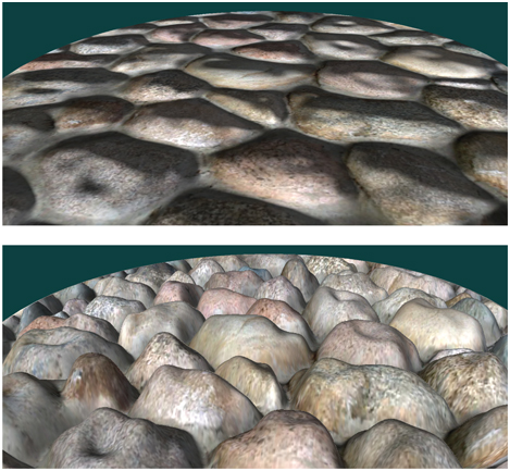
Figure 6.41. Normal mapping and relief mapping. No self-occlusion occurs with normal mapping. Relief mapping has problems with silhouettes for repeating textures, as the rectangle is more of a view into the heightfield than a true boundary definition. (Images courtesy of NVIDIA Corporation.)
Another approach to increasing both performance and sampling accuracy is to not initially sample the heightfield at a regular interval, but instead to try to skip intervening empty space. Donnelly [367] preprocesses the height field into a set of voxels, storing in each voxel how far away it is from the heightfield surface. In this way, intervening space can be rapidly skipped, at the cost of higher storage for each heightfield. Wang et al. [1844] use a five-dimensional displacement mapping scheme to hold distances to the surface from all directions and locations. This allows complex curved surfaces, self-shadowing, and other effects, at the expense of considerably larger amounts of memory. Mehra and Kumar [1195] use directional distance maps for similar purposes. Dummer [393] introduces, and Policarpo and Oliveira [1426] improve upon, the idea of cone step mapping. The concept here is to also store for each heightfield location a cone radius. This radius defines an interval on the ray in which there is at most one intersection with the heightfield. This property allows rapid skipping along the ray without missing any possible intersections, though at the cost of needing dependent texture reads. Another drawback is the precomputation needed to create the cone step map, making the method unusable for dynamically changing heightfields. Schroders and Gulik [1581] present quadtree relief mapping, a hierarchical method to skip over volumes during traversal. Tevs et al. [1760] use “maximum mipmaps” to allow skipping while minimizing precomputation costs. Drobot [377] also uses a quadtree-like structure stored in mipmaps to speed up traversal, and presents a method to blend between different heightfields, where one terrain type transitions to another.
One problem with all the methods above is that the illusion breaks down along the silhouette edges of objects, which will show the original surface’s smooth outlines. See Figure 6.41.

Figure 6.42. Parallax occlusion mapping, a.k.a. relief mapping, used on a path to make the stones look more realistic. The ground is actually a simple set of triangles with a heightfield applied. (Image from “Crysis,” courtesy of Crytek.)
The key idea is that the triangles rendered define which pixels should be evaluated by the pixel shader program, not where the surface actually is located. In addition, for curved surfaces, the problem of silhouettes becomes more involved. One approach is described and developed by Oliveira and Policarpo [1325,1850], which uses a quadratic silhouette approximation technique. Jeschke et al. [824] and Dachsbacher et al. [323] both give a more general and robust method (and review previous work) for dealing with silhouettes and curved surfaces correctly. First explored by Hirche [750], the general idea is to extrude each triangle in the mesh outward and form a prism. Rendering this prism forces evaluation of all pixels in which the heightfield could possibly appear. This type of approach is called shell mapping, as the expanded mesh forms a separate shell over the original model. By preserving the nonlinear nature of prisms when intersecting them with rays, artifact-free rendering of heightfields becomes possible, though expensive to compute. An impressive use of this type of technique is shown in Figure 6.42.
6.9 Textured Lights
Textures can also be used to add visual richness to light sources and allow for complex intensity distribution or spotlight functions. For lights that have all their illumination limited to a cone or frustum, projective textures can be used to modulate the light intensity [1192,1597,1904]. This allows for shaped spotlights, patterned lights, and even “slide projector” effects (Figure 6.43). These lights are often called gobo or cookie lights, after the terms for the cutouts used in professional theater and film lighting.

Figure 6.43. Projective textured light. The texture is projected onto the teapot and ground plane and used to modulate the light’s contribution within the projection frustum (it is set to 0 outside the frustum). (Image courtesy of NVIDIA Corporation.)
See Section 7.2 for a discussion of projective mapping being used in a similar way to cast shadows.
For lights that are not limited to a frustum but illuminate in all directions, a cube map can be used to modulate the intensity, instead of a two-dimensional projective texture. One-dimensional textures can be used to define arbitrary distance falloff functions. Combined with a two-dimensional angular attenuation map, this can allow for complex volumetric lighting patterns [353]. A more general possibility is to use three-dimensional (volume) textures to control the light’s falloff [353,535,1192]. This allows for arbitrary volumes of effect, including light beams. This technique is memory intensive (as are all volume textures). If the light’s volume of effect is symmetrical along the three axes, the memory footprint can be reduced eightfold by mirroring the data into each octant.
Textures can be added to any light type to enable additional visual effects. Textured lights allow for easy control of the illumination by artists, who can simply edit the texture used.
Further Reading and Resources
Heckbert has written a good survey of the theory of texture mapping [690] and a more in-depth report on the topic [691]. Szirmay-Kalos and Umenhoffer [1731] have an excellent, thorough survey of parallax occlusion mapping and displacement methods. More information about normal representation can be found in the work by Cigolle et al. [269] and by Meyer et al. [1205].
The book Advanced Graphics Programming Using OpenGL [1192] has extensive coverage of various visualization techniques using texturing algorithms. For extensive coverage of three-dimensional procedural textures, see Texturing and Modeling: A Procedural Approach [407]. The book Advanced Game Development with Programmable Graphics Hardware [1850] has many details about implementing parallax occlusion mapping techniques, as do Tatarchuk’s presentations [1742,1743] and Szirmay-Kalos and Umenhoffer’s survey [1731].
For procedural texturing (and modeling), our favorite site on the Internet is Shadertoy. There are many worthwhile and fascinating procedural texturing functions on display, and you can easily modify any example and see the results.
Visit this book’s website, http://www.w3.org/1999/xlink, for many other resources.
1 An alternate DXT1 mode reserves one of the four possible interpolation factors for transparent pixels, restricting the number of interpolated values to three—the two reference values and their average.