
Chapter 7
Shadows
“All the variety, all the charm, all the beauty of life is made up of light and shadow.”
—Tolstoy
Shadows are important for creating realistic images and in providing the user with visual cues about object placement. This chapter focuses on the basic principles of computing shadows, and describes the most important and popular real-time algorithms for doing so. We also briefly discuss approaches that are less popular but embody important principles. We do not spend time in this chapter covering all options and approaches, as there are two comprehensive books that study the field of shadows in great depth [412, 1902]. Instead, we focus on surveying articles and presentations that have appeared since their publication, with a bias toward battle-tested techniques.
The terminology used throughout this chapter is illustrated in Figure 7.1, where occluders are objects that cast shadows onto receivers. Punctual light sources, i.e., those with no area, generate only fully shadowed regions, sometimes called hard shadows. If area or volume light sources are used, then soft shadows are produced. Each shadow can then have a fully shadowed region, called the umbra, and a partially shadowed region, called the penumbra. Soft shadows are recognized by their fuzzy shadow edges. However, it is important to note that they generally cannot be rendered correctly by just blurring the edges of a hard shadow with a low-pass filter. As can be seen in Figure 7.2, a correct soft shadow is sharper the closer the shadow-casting geometry is to the receiver. The umbra region of a soft shadow is not equivalent to a hard shadow generated by a punctual light source. Instead, the umbra region of a soft shadow decreases in size as the light source grows larger, and it might even disappear, given a large enough light source and a receiver far enough from the occluder. Soft shadows are generally preferable because the penumbrae edges let the viewer know that the shadow is indeed a shadow. Hard-edged shadows usually look less realistic and can sometimes be misinterpreted as actual geometric features, such as a crease in a surface. However, hard shadows are faster to render than soft shadows.

Figure 7.1 Shadow terminology: light source, occluder, receiver, shadow, umbra, and penumbra.

Figure 7.2 A mix of hard and soft shadows. Shadows from the crate are sharp, as the occluder is near the receiver. The person’s shadow is sharp at the point of contact, softening as the distance to the occluder increases. The distant tree branches give soft shadows [1711]. (Image from “Tom Clancy’s The Division,” courtesy of Ubisoft.)
More important than having a penumbra is having any shadow at all. Without some shadow as a visual cue, scenes are often unconvincing and more difficult to perceive. As Wanger shows [1846], it is usually better to have an inaccurate shadow than none at all, as the eye is fairly forgiving about the shadow’s shape. For example, a blurred black circle applied as a texture on the floor can anchor a character to the ground.
In the following sections, we will go beyond these simple modeled shadows and present methods that compute shadows automatically in real time from the occluders in a scene. The first section handles the special case of shadows cast on planar surfaces, and the second section covers more general shadow algorithms, i.e., casting shadows onto arbitrary surfaces. Both hard and soft shadows will be covered. To conclude, some optimization techniques are presented that apply to various shadow algorithms.
7.1 Planar Shadows
A simple case of shadowing occurs when objects cast shadows onto a planar surface. A few types of algorithms for planar shadows are presented in this section, each with variations in the softness and realism of the shadows.
7.1.1 Projection Shadows
In this scheme, the three-dimensional object is rendered a second time to create a shadow. A matrix can be derived that projects the vertices of an object onto a plane [162, 1759]. Consider the situation in Figure 7.3, where the light source is located at l, the vertex to be projected is at v, and the projected vertex is at p. We will derive the projection matrix for the special case where the shadowed plane is y = 0, and then this result will be generalized to work with any plane.

Figure 7.3 Left: A light source, located at l, casts a shadow onto the plane y = 0. The vertex v is projected onto the plane. The projected point is called p. The similar triangles are used for the derivation of the projection matrix. Right: The shadow is being cast onto a plane, π : n · x + d = 0.
We start by deriving the projection for the x-coordinate. From the similar triangles in the left part of Figure 7.3, we get
(7.1)
The z-coordinate is obtained in the same way: p z = (l y v z − l z v y)/(l y − v y), while the y-coordinate is zero. Now these equations can be converted into the projection matrix M:
(7.2)
It is straightforward to verify that Mv = p, which means that M is indeed the projection matrix.
In the general case, the plane onto which the shadows should be cast is not the plane y = 0, but instead π : n · x + d = 0. This case is depicted in the right part of Figure 7.3. The goal is again to find a matrix that projects v down to p. To this end, the ray emanating at l, which goes through v, is intersected by the plane π. This yields the projected point p:
(7.3)
This equation can also be converted into a projection matrix, shown in Equation 7.4, which satisfies Mv = p:
(7.4)
As expected, this matrix turns into the matrix in Equation 7.2 if the plane is y = 0, that is, n = (0, 1, 0) and d = 0.
To render the shadow, simply apply this matrix to the objects that should cast shadows on the plane π, and render this projected object with a dark color and no illumination. In practice, you have to take measures to avoid allowing the projected triangles to be rendered beneath the surface receiving them. One method is to add some bias to the plane we project upon, so that the shadow triangles are always rendered in front of the surface.
A safer method is to draw the ground plane first, then draw the projected triangles with the z-buffer off, then render the rest of the geometry as usual. The projected triangles are then always drawn on top of the ground plane, as no depth comparisons are made.
If the ground plane has a limit, e.g., it is a rectangle, the projected shadows may fall outside of it, breaking the illusion. To solve this problem, we can use a stencil buffer. First, draw the receiver to the screen and to the stencil buffer. Then, with the z-buffer off, draw the projected triangles only where the receiver was drawn, then render the rest of the scene normally.
Another shadow algorithm is to render the triangles into a texture, which is then applied to the ground plane. This texture is a type of light map, a texture that modulates the intensity of the underlying surface (Section 11.5.1). As will be seen, this idea of rendering the shadow projection to a texture also allows penumbrae and shadows on curved surfaces. One drawback of this technique is that the texture can become magnified, with a single texel covering multiple pixels, breaking the illusion.
If the shadow situation does not change from frame to frame, i.e., the light and shadow casters do not move relative to each other, this texture can be reused. Most shadow techniques can benefit from reusing intermediate computed results from frame to frame if no change has occurred.
All shadow casters must be between the light and the ground-plane receiver. If the light source is below the topmost point on the object, an antishadow [162] is generated, since each vertex is projected through the point of the light source. Correct shadows and antishadows are shown in Figure 7.4. An error will also occur if we project an object that is below the receiving plane, since it too should cast no shadow.
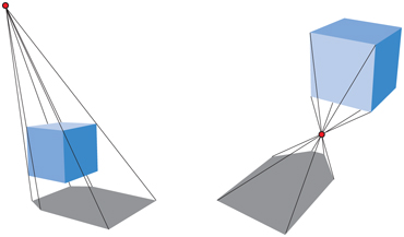
Figure 7.4 At the left, a correct shadow is shown, while in the figure on the right, an antishadow appears, since the light source is below the topmost vertex of the object.
It is certainly possible to explicitly cull and trim shadow triangles to avoid such artifacts. A simpler method, presented next, is to use the existing GPU pipeline to perform projection with clipping.
7.1.2 Soft Shadows
Projective shadows can also be made soft, by using a variety of techniques. Here, we describe an algorithm from Heckbert and Herf [697, 722] that produces soft shadows. The algorithm’s goal is to generate a texture on a ground plane that shows a soft shadow. We then describe less accurate, faster methods.
Soft shadows appear whenever a light source has an area. One way to approximate the effect of an area light is to sample it by using several punctual lights placed on its surface. For each of these punctual light sources, an image is rendered and accumulated into a buffer. The average of these images is then an image with soft shadows. Note that, in theory, any algorithm that generates hard shadows can be used along with this accumulation technique to produce penumbrae. In practice, doing so at interactive rates is usually untenable because of the execution time that would be involved.
Heckbert and Herf use a frustum-based method to produce their shadows. The idea is to treat the light as the viewer, and the ground plane forms the far clipping plane of the frustum. The frustum is made wide enough to encompass the occluders. A soft shadow texture is formed by generating a series of ground-plane textures.
The area light source is sampled over its surface, with each location used to shade the image representing the ground plane, then to project the shadow-casting objects onto this image. All these images are summed and averaged to produce a ground-plane shadow texture. See the left side of Figure 7.5 for an example.
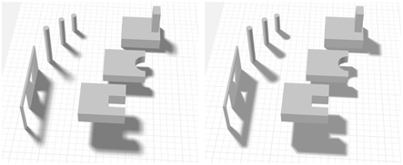
Figure 7.5 On the left, a rendering using Heckbert and Herf’s method, using 256 passes. On the right, Haines’ method in one pass. The umbrae are too large with Haines’ method, which is particularly noticeable around the doorway and window.
A problem with the sampled area-light method is that it tends to look like what it is: several overlapping shadows from punctual light sources. Also, for n shadow passes, only n + 1 distinct shades can be generated. A large number of passes gives an accurate result, but at an excessive cost. The method is useful for obtaining a (literally) “ground-truth” image for testing the quality of other, faster algorithms.
A more efficient approach is to use convolution, i.e., filtering. Blurring a hard shadow generated from a single point can be sufficient in some cases and can produce a semitransparent texture that can be composited with real-world content. See Figure 7.6. However, a uniform blur can be unconvincing near where the object makes contact with the ground.

Figure 7.6 Drop shadow. A shadow texture is generated by rendering the shadow casters from above and then blurring the image and rendering it on the ground plane. (Image generated in Autodesk’s A360 viewer, model from Autodesk’s Inventor samples.)
There are many other methods that give a better approximation, at additional cost. For example, Haines [644] starts with a projected hard shadow and then renders the silhouette edges with gradients that go from dark in the center to white on the edges to create plausible penumbrae. See the right side of Figure 7.5. However, these penumbrae are not physically correct, as they should also extend to areas inside the silhouette edges. Iwanicki [356, 806] draws on ideas from spherical harmonics and approximates occluding characters with ellipsoids to give soft shadows. All such methods have various approximations and drawbacks, but are considerably more efficient than averaging a large set of drop-shadow images.
7.2 Shadows on Curved Surfaces
One simple way to extend the idea of planar shadows to curved surfaces is to use a generated shadow image as a projective texture [1192, 1254, 1272, 1597]. Think of shadows from the light’s point of view. Whatever the light sees is illuminated; what it does not see is in shadow. Say the occluder is rendered in black from the light’s viewpoint into an otherwise white texture. This texture can then be projected onto the surfaces that are to receive the shadow. Effectively, each vertex on the receivers has a (u, v) texture coordinate computed for it and has the texture applied to it. These texture coordinates can be computed explicitly by the application. This differs a bit from the ground shadow texture in the previous section, where objects are projected onto a specific physical plane. Here, the image is made as a view from the light, like a frame of film in a projector.
When rendered, the projected shadow texture modifies the receiver surfaces. It can also be combined with other shadow methods, and sometimes is used primarily for helping aid perception of an object’s location. For example, in a platform-hopping video game, the main character might always be given a drop shadow directly below it, even when the character is in full shadow [1343]. More elaborate algorithms can give better results. For example, Eisemann and D′ecoret [411] assume a rectangular overhead light and create a stack of shadow images of horizontal slices of the object, which are then turned into mipmaps or similar. The corresponding area of each slice is accessed proportional to its distance from the receiver by using its mipmap, meaning that more distant slices will cast softer shadows.
There are some serious drawbacks of texture projection methods. First, the application must identify which objects are occluders and which are their receivers. The receiver must be maintained by the program to be further from the light than the occluder, otherwise the shadow is “cast backward.” Also, occluding objects cannot shadow themselves. The next two sections present algorithms that generate correct shadows without the need for such intervention or limitations.
Note that a variety of lighting patterns can be obtained by using prebuilt projective textures. A spotlight is simply a square projected texture with a circle inside of it defining the light. A Venetian blinds effect can be created by a projected texture consisting of horizontal lines. This type of texture is called a light attenuation mask, cookie texture, or gobo map. A prebuilt pattern can be combined with a projected texture created on the fly by simply multiplying the two textures together. Such lights are discussed further in Section 6.9.
7.3 Shadow Volumes
Presented by Heidmann in 1991 [701], a method based on Crow’s shadow volumes [311] can cast shadows onto arbitrary objects by clever use of the stencil buffer. It can be used on any GPU, as the only requirement is a stencil buffer. It is not image based (unlike the shadow map algorithm described next) and so avoids sampling problems, thus producing correct sharp shadows everywhere. This can sometimes be a disadvantage. For example, a character’s clothing may have folds that give thin, hard shadows that alias badly. Shadow volumes are rarely used today, due to their unpredictable cost [1599]. We give the algorithm a brief description here, as it illustrates some important principles and research based on these continues.
To begin, imagine a point and a triangle. Extending the lines from a point through the vertices of a triangle to infinity yields an infinite three-sided pyramid. The part under the triangle, i.e., the part that does not include the point, is a truncated infinite pyramid, and the upper part is simply a pyramid. This is illustrated in Figure 7.7. Now imagine that the point is actually a point light source. Then, any part of an object that is inside the volume of the truncated pyramid (under the triangle) is in shadow. This volume is called a shadow volume.

Figure 7.7 Left: the lines from a point light are extended through the vertices of a triangle to form an infinite pyramid. Right: the upper part is a pyramid, and the lower part is an infinite truncated pyramid, also called the shadow volume. All geometry that is inside the shadow volume is in shadow.
Say we view some scene and follow a ray from the eye through a pixel until the ray hits the object to be displayed on screen. While the ray is on its way to this object, we increment a counter each time it crosses a face of the shadow volume that is frontfacing (i.e., facing toward the viewer). Thus, the counter is incremented each time the ray goes into shadow. In the same manner, we decrement the same counter each time the ray crosses a backfacing face of the truncated pyramid. The ray is then going out of a shadow. We proceed, incrementing and decrementing the counter until the ray hits the object that is to be displayed at that pixel. If the counter is greater than zero, then that pixel is in shadow; otherwise it is not. This principle also works when there is more than one triangle that casts shadows. See Figure 7.8.
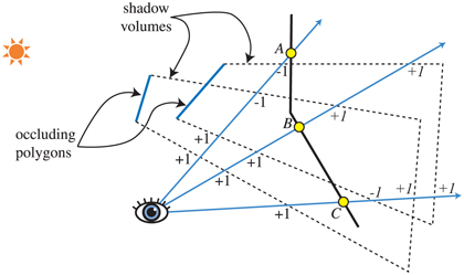
Figure 7.8 A two-dimensional side view of counting shadow-volume crossings using two different counting methods. In z-pass volume counting, the count is incremented as a ray passes through a frontfacing triangle of a shadow volume and decremented on leaving through a backfacing triangle. So, at point A, the ray enters two shadow volumes for +2, then leaves two volumes, leaving a net count of zero, so the point is in light. In z-fail volume counting, the count starts beyond the surface (these counts are shown in italics). For the ray at point B, the z-pass method gives a +2 count by passing through two frontfacing triangles, and the z-fail gives the same count by passing through two backfacing triangles. Point C shows how z-fail shadow volumes must be capped. The ray starting from point C first hits a frontfacing triangle, giving −1. It then exits two shadow volumes (through their endcaps, necessary for this method to work properly), giving a net count of +1. The count is not zero, so the point is in shadow. Both methods always give the same count results for all points on the viewed surfaces.
Doing this with rays is time consuming. But there is a much smarter solution [701]: A stencil buffer can do the counting for us. First, the stencil buffer is cleared. Second, the whole scene is drawn into the framebuffer with only the color of the unlit material used, to get these shading components in the color buffer and the depth information into the z-buffer. Third, z-buffer updates and writing to the color buffer are turned off (though z-buffer testing is still done), and then the frontfacing triangles of the shadow volumes are drawn. During this process, the stencil operation is set to increment the values in the stencil buffer wherever a triangle is drawn. Fourth, another pass is done with the stencil buffer, this time drawing only the backfacing triangles of the shadow volumes. For this pass, the values in the stencil buffer are decremented when the triangles are drawn. Incrementing and decrementing are done only when the pixels of the rendered shadow-volume face are visible (i.e., not hidden by any real geometry). At this point the stencil buffer holds the state of shadowing for every pixel. Finally, the whole scene is rendered again, this time with only the components of the active materials that are affected by the light, and displayed only where the value in the stencil buffer is 0. A value of 0 indicates that the ray has gone out of shadow as many times as it has gone into a shadow volume—i.e., this location is illuminated by the light. This counting method is the basic idea behind shadow volumes. An example of shadows generated by the shadow volume algorithm is shown in Figure 7.9. There are efficient ways to implement the algorithm in a single pass [1514]. However, counting problems will occur when an object penetrates the camera’s near plane. The solution, called z-fail, involves counting the crossings hidden behind visible surfaces instead of in front [450, 775]. A brief summary of this alternative is shown in Figure 7.8.

Figure 7.9 Shadow volumes. On the left, a character casts a shadow. On the right, the extruded triangles of the model are shown. (Images from Microsoft SDK [1208] sample “ShadowVolume.”)
Creating quadrilaterals for every triangle creates a huge amount of overdraw. That is, each triangle will create three quadrilaterals that must be rendered. A sphere triangles are drawn. Incrementing and decrementing are done only when the pixels of the rendered shadow-volume face are visible (i.e., not hidden by any real geometry). At this point the stencil buffer holds the state of shadowing for every pixel. Finally, the whole scene is rendered again, this time with only the components of the active materials that are affected by the light, and displayed only where the value in the stencil buffer is 0. A value of 0 indicates that the ray has gone out of shadow as many times as it has gone into a shadow volume—i.e., this location is illuminated by the light. This counting method is the basic idea behind shadow volumes. An example of shadows generated by the shadow volume algorithm is shown in Figure 7.9. There are efficient ways to implement the algorithm in a single pass [1514]. However, counting problems will occur when an object penetrates the camera’s near plane. The solution, called z-fail, involves counting the crossings hidden behind visible surfaces instead of in front [450, 775]. A brief summary of this alternative is shown in Figure 7.8.
Creating quadrilaterals for every triangle creates a huge amount of overdraw. That is, each triangle will create three quadrilaterals that must be rendered. A sphere made of a thousand triangles creates three thousand quadrilaterals, and each of those quadrilaterals may span the screen. One solution is to draw only those quadrilaterals along the silhouette edges of the object, e.g., our sphere may have only fifty silhouette edges, so only fifty quadrilaterals are needed. The geometry shader can be used to automatically generate such silhouette edges [1702]. Culling and clamping techniques can also be used to lower fill costs [1061].
However, the shadow volume algorithm still has a terrible drawback: extreme variability. Imagine a single, small triangle in view. If the camera and the light are in exactly the same position, the shadow-volume cost is minimal. The quadrilaterals formed will not cover any pixels as they are edge-on to the view. Only the triangle itself matters. Say the viewer now orbits around the triangle, keeping it in view. As the camera moves away from the light source, the shadow-volume quadrilaterals will become more visible and cover more of the screen, causing more computation to occur. If the viewer should happen to move into the shadow of the triangle, the shadow volume will entirely fill the screen, costing a considerable amount of time to evaluate compared to our original view. This variability is what makes shadow volumes unusable in interactive applications where a consistent frame rate is important. Viewing toward the light can cause huge, unpredictable jumps in the cost of the algorithm, as can other scenarios.
For these reasons shadow volumes have been for the most part abandoned by applications. However, given the continuing evolution of new and different ways to access data on the GPU, and the clever repurposing of such functionality by researchers, shadow volumes may someday come back into general use. For example, Sintorn et al. [1648] give an overview of shadow-volume algorithms that improve efficiency and propose their own hierarchical acceleration structure.
The next algorithm presented, shadow mapping, has a much more predictable cost and is well suited to the GPU, and so forms the basis for shadow generation in many applications.
7.4 Shadow Maps
In 1978, Williams [1888] proposed that a common z-buffer-based renderer could be used to generate shadows quickly on arbitrary objects. The idea is to render the scene, using the z-buffer, from the position of the light source that is to cast shadows. Whatever the light “sees” is illuminated, the rest is in shadow. When this image is generated, only z-buffering is required. Lighting, texturing, and writing values into the color buffer can be turned off.
Each pixel in the z-buffer now contains the z-depth of the object closest to the light source. We call the entire contents of the z-buffer the shadow map, also sometimes known as the shadow depth map or shadow buffer. To use the shadow map, the scene is rendered a second time, but this time with respect to the viewer. As each drawing primitive is rendered, its location at each pixel is compared to the shadow map. If a rendered point is farther away from the light source than the corresponding value in the shadow map, that point is in shadow, otherwise it is not. This technique is implemented by using texture mapping. See Figure 7.10. Shadow mapping is a popular algorithm because it is relatively predictable. The cost of building the shadow map is roughly linear with the number of rendered primitives, and access time is constant. The shadow map can be generated once and reused each frame for scenes where the light and objects are not moving, such as for computer-aided design.

Figure 7.10 Shadow mapping. On the top left, a shadow map is formed by storing the depths to the surfaces in view. On the top right, the eye is shown looking at two locations. The sphere is seen at point va, and this point is found to be located at texel a on the shadow map. The depth stored there is not (much) less than point va is from the light, so the point is illuminated. The rectangle hit at point vb is (much) farther away from the light than the depth stored at texel b, and so is in shadow. On the bottom left is the view of a scene from the light’s perspective, with white being farther away. On the bottom right is the scene rendered with this shadow map.
When a single z-buffer is generated, the light can “look” in only a particular direction, like a camera. For a distant directional light such as the sun, the light’s view is set to encompass all objects casting shadows into the viewing volume that the eye sees. The light uses an orthographic projection, and its view needs to be made wide and high enough in x and y to view this set of objects. Local light sources need similar adjustments, as possible. If the local light is far enough away from the shadow-casting objects, a single view frustum may be sufficient to encompass all of these. Alternately, if the local light is a spotlight, it has a natural frustum associated with it, with everything outside its frustum considered not illuminated.
If the local light source is inside a scene and is surrounded by shadow-casters, a typical solution is to use a six-view cube, similar to cubic environment mapping [865]. These are called omnidirectional shadow maps. The main challenge for omnidirectional maps is avoiding artifacts along the seams where two separate maps meet. King and Newhall [895] analyze the problems in depth and provide solutions, and Gerasimov [525] provides some implementation details. Forsyth [484, 486] presents a general multi-frustum partitioning scheme for omnidirectional lights that also provides more shadow map resolution where needed. Crytek [1590, 1678, 1679] sets the resolution of each of the six views for a point light based on the screen-space coverage of each view’s projected frustum, with all maps stored in a texture atlas.
Not all objects in the scene need to be rendered into the light’s view volume. First, only objects that can cast shadows need to be rendered. For example, if it is known that the ground can only receive shadows and not cast one, then it does not have to be rendered into the shadow map.
Shadow casters are by definition those inside the light’s view frustum. This frustum can be augmented or tightened in several ways, allowing us to safely disregard some shadow casters [896, 1812]. Think of the set of shadow receivers visible to the eye. This set of objects is within some maximum distance along the light’s view direction. Anything beyond this distance cannot cast a shadow on the visible receivers. Similarly, the set of visible receivers may well be smaller than the light’s original x and y view bounds. See Figure 7.11. Another example is that if the light source is inside the eye’s view frustum, no object outside this additional frustum can cast a shadow on a receiver. Rendering only relevant objects not only can save time rendering, but can also reduce the size required for the light’s frustum and so increase the effective resolution of the shadow map, thus improving quality. In addition, it helps if the light frustum’s near plane is as far away from the light as possible, and if the far plane is as close as possible. Doing so increases the effective precision of the z-buffer [1792] (Section 4.7.2).

Figure 7.11 On the left, the light’s view encompasses the eye’s frustum. In the middle, the light’s far plane is pulled in to include only visible receivers, so culling the triangle as a caster; the near plane is also adjusted. On the right, the light’s frustum sides are made to bound the visible receivers, culling the green capsule.
One disadvantage of shadow mapping is that the quality of the shadows depends on the resolution (in pixels) of the shadow map and on the numerical precision of the z-buffer. Since the shadow map is sampled during the depth comparison, the algorithm is susceptible to aliasing problems, especially close to points of contact between objects. A common problem is self-shadow aliasing, often called “surface acne” or “shadow acne,” in which a triangle is incorrectly considered to shadow itself. This problem has two sources. One is simply the numerical limits of precision of the processor. The other source is geometric, from the fact that the value of a point sample is being used to represent an area’s depth. That is, samples generated for the light are almost never at the same locations as the screen samples (e.g., pixels are often sampled at their centers). When the light’s stored depth value is compared to the viewed surface’s depth, the light’s value may be slightly lower than the surface’s, resulting in self-shadowing. The effects of such errors are shown in Figure 7.12.

Figure 7.12 Shadow-mapping bias artifacts. On the left, the bias is too low, so self-shadowing occurs. On the right, a high bias causes the shoes to not cast contact shadows. The shadow-map resolution is also too low, giving the shadow a blocky appearance. (Images generated using a shadow demo by Christoph Peters.)
One common method to help avoid (but not always eliminate) various shadow-map artifacts is to introduce a bias factor. When checking the distance found in the shadow map with the distance of the location being tested, a small bias is subtracted from the receiver’s distance. See Figure 7.13. This bias could be a constant value [1022], but doing so can fail when the receiver is not mostly facing the light. A more effective method is to use a bias that is proportional to the angle of the receiver to the light. The more the surface tilts away from the light, the greater the bias grows, to avoid the problem. This type of bias is called the slope scale bias. Both biases can be applied by using a command such as OpenGL’s glPolygonOffset) to shift each polygon away from the light. Note that if a surface directly faces the light, it is not biased backward at all by slope scale bias. For this reason, a constant bias is used along with slope scale bias to avoid possible precision errors. Slope scale bias is also often clamped at some maximum, since the tangent value can be extremely high when the surface is nearly edge-on when viewed from the light.

Figure 7.13 Shadow bias. The surfaces are rendered into a shadow map for an overhead light, with the vertical lines representing shadow-map pixel centers. Occluder depths are recorded at the × locations. We want to know if the surface is lit at the three samples shown as dots. The closest shadow-map depth value for each is shown with the same color ×. On the left, if no bias is added, the blue and orange samples will be incorrectly determined to be in shadow, since they are farther from the light than their corresponding shadow-map depths. In the middle, a constant depth bias is subtracted from each sample, placing each closer to the light. The blue sample is still considered in shadow because it is not closer to the light than the shadow-map depth it is tested against. On the right, the shadow map is formed by moving each polygon away from the light proportional to its slope. All sample depths are now closer than their shadow-map depths, so all are lit.
Holbert [759, 760] introduced normal offset bias, which first shifts the receiver’s world-space location a bit along the surface’s normal direction, proportional to the sine of the angle between the light’s direction and the geometric normal. See Figure 7.24 on page 250. This changes not only the depth but also the xand y-coordinates where the sample is tested on the shadow map. As the light’s angle becomes more shallow to the surface, this offset is increased, in hopes that the sample becomes far enough above the surface to avoid self-shadowing. This method can be visualized as moving the sample to a “virtual surface” above the receiver. This offset is a worldspace distance, so Pettineo [1403] recommends scaling it by the depth range of the shadow map. Pesce [1391] suggests the idea of biasing along the camera view direction, which also works by adjusting the shadow-map coordinates. Other bias methods are discussed in Section 7.5, as the shadow method presented there needs to also test several neighboring samples.
Too much bias causes a problem called light leaks or Peter Panning, in which the object appears to float slightly above the underlying surface. This artifact occurs because the area beneath the object’s point of contact, e.g., the ground under a foot, is pushed too far forward and so does not receive a shadow.
One way to avoid self-shadowing problems is to render only the backfaces to the shadow map. Called second-depth shadow mapping [1845], this scheme works well for many situations, especially for a rendering system where hand-tweaking a bias is not an option. The problem cases occur when objects are two-sided, thin, or in contact with one another. If an object is a model where both sides of the mesh are visible, e.g., a palm frond or sheet of paper, self-shadowing can occur because the backface and the frontface are in the same location. Similarly, if no biasing is performed, problems can occur near silhouette edges or thin objects, since in these areas backfaces are close to frontfaces. Adding a bias can help avoid surface acne, but the scheme is more susceptible to light leaking, as there is no separation between the receiver and the backfaces of the occluder at the point of contact. See Figure 7.14. Which scheme to choose can be situation dependent. For example, Sousa et al. [1679] found using frontfaces for sun shadows and backfaces for interior lights to work best for their applications.

Figure 7.14 Shadow-map surfaces for an overhead light source. On the left, surfaces facing the light, marked in red, are sent to the shadow map. Surfaces may be incorrectly determined to shadow themselves (“acne”), so need to be biased away from the light. In the middle, only the backfacing triangles are rendered into the shadow map. A bias pushing these occluders downward could let light leak onto the ground plane near location a; a bias forward can cause illuminated locations near the silhouette boundaries marked b to be considered in shadow. On the right, an intermediate surface is formed at the midpoints between the closest frontand backfacing triangles found at each location on the shadow map. A light leak can occur near point c (which can also happen with second-depth shadow mapping), as the nearest shadow-map sample may be on the intermediate surface to the left of this location, and so the point would be closer to the light.
Note that for shadow mapping, objects must be “watertight” (manifold and closed, i.e., solid; Section 16.3.3), or must have both frontand backfaces rendered to the map, else the object may not fully cast a shadow. Woo [1900] proposes a general method that attempts to, literally, be a happy medium between using just frontfaces or backfaces for shadowing. The idea is to render solid objects to a shadow map and keep track of the two closest surfaces to the light. This process can be performed by depth peeling or other transparency-related techniques. The average depth between the two objects forms an intermediate layer whose depth is used as a shadow map, sometimes called a dual shadow map [1865]. If the object is thick enough, self-shadowing and light-leak artifacts are minimized. Bavoil et al. [116] discuss ways to address potential artifacts, along with other implementation details. The main drawbacks are the additional costs associated with using two shadow maps. Myers [1253] discusses an artist-controlled depth layer between the occlude and receiver.
As the viewer moves, the light’s view volume often changes size as the set of shadow casters changes. Such changes in turn cause the shadows to shift slightly from frame to frame. This occurs because the light’s shadow map is sampling a different set of directions from the light, and these directions are not aligned with the previous set. For directional lights, the solution is to force each succeeding shadow map generated to maintain the same relative texel beam locations in world space [927, 1227, 1792, 1810]. That is, you can think of the shadow map as imposing a two-dimensional gridded frame of reference on the whole world, with each grid cell representing a pixel sample on the map. As you move, the shadow map is generated for a different set of these same grid cells. In other words, the light’s view projection is forced to this grid to maintain frame to frame coherence.
7.4.1 Resolution Enhancement
Similar to how textures are used, ideally we want one shadow-map texel to cover about one image pixel. If we have a light source located at the same position as the eye, the shadow map perfectly maps one-to-one with the screen-space pixels (and there are no visible shadows, since the light illuminates exactly what the eye sees). As soon as the light’s direction changes, this per-pixel ratio changes, which can cause artifacts. An example is shown in Figure 7.15. The shadow is blocky and poorly defined because a large number of pixels in the foreground are associated with each texel of the shadow map. This mismatch is called perspective aliasing. Single shadow-map texels can also cover many pixels if a surface is nearly edge-on to the light, but faces the viewer. This problem is known as projective aliasing [1792]; see Figure 7.16. Blockiness can be decreased by increasing the shadow-map resolution, but at the cost of additional memory and processing.

Figure 7.15 The image to the left is created using standard shadow mapping; the image to the right using LiSPSM. The projections of each shadow map’s texels are shown. The two shadow maps have the same resolution, the di_erence being that LiSPSM reforms the light’s matrices to provide a higher sampling rate nearer the viewer. (Images courtesy of Daniel Scherzer, Vienna University of Technology.)

Figure 7.16 On the left the light is nearly overhead. The edge of the shadow is a bit ragged due to a low resolution compared to the eye’s view. On the right the light is near the horizon, so each shadow texel covers considerably more screen area horizontally and so gives a more jagged edge. (Images generated by TheRealMJP’s “Shadows” program on Github.)
There is another approach to creating the light’s sampling pattern that makes it more closely resemble the camera’s pattern. This is done by changing the way the scene projects toward the light. Normally we think of a view as being symmetric, with the view vector in the center of the frustum. However, the view direction merely defines a view plane, but not which pixels are sampled. The window defining the frustum can be shifted, skewed, or rotated on this plane, creating a quadrilateral that gives a different mapping of world to view space. The quadrilateral is still sampled at regular intervals, as this is the nature of a linear transform matrix and its use by the GPU. The sampling rate can be modified by varying the light’s view direction and the view window’s bounds. See Figure 7.17.

Figure 7.17 For an overhead light, on the left the sampling on the floor does not match the eye’s rate. By changing the light’s view direction and projection window on the right, the sampling rate is biased toward having a higher density of texels nearer the eye.
There are 22 degrees of freedom in mapping the light’s view to the eye’s [896]. Exploration of this solution space led to several different algorithms that attempt to better match the light’s sampling rates to the eye’s. Methods include perspective shadow maps (PSM) [1691], trapezoidal shadow maps (TSM) [1132], and light space perspective shadow maps (LiSPSM) [1893, 1895]. See Figure 7.15 and Figure 7.26 on page 254 for examples. Techniques in this class are referred to as perspective warping methods.
An advantage of these matrix-warping algorithms is that no additional work is needed beyond modifying the light’s matrices. Each method has its own strengths and weaknesses [484], as each can help match sampling rates for some geometry and lighting situations, while worsening these rates for others. Lloyd et al. [1062, 1063] analyze the equivalences between PSM, TSM, and LiSPSM, giving an excellent overview of the sampling and aliasing issues with these approaches. These schemes work best when the light’s direction is perpendicular to the view’s direction (e.g., overhead), as the perspective transform can then be shifted to put more samples closer to the eye.
One lighting situation where matrix-warping techniques fail to help is when a light is in front of the camera and pointing at it. This situation is known as dueling frusta, or more colloquially as “deer in the headlights.” More shadow-map samples are needed nearer the eye, but linear warping can only make the situation worse [1555]. This and other problems, such as sudden changes in quality [430] and a “nervous,” unstable quality to the shadows produced during camera movement [484, 1227], have made these approaches fall out of favor.
The idea of adding more samples where the viewer is located is a good one, leading to algorithms that generate several shadow maps for a given view. This idea first made a noticeable impact when Carmack described it at his keynote at Quakecon 2004. Blow independently implemented such a system [174]. The idea is simple: Generate a fixed set of shadow maps (possibly at different resolutions), covering different areas of the scene. In Blow’s scheme, four shadow maps are nested around the viewer. In this way, a high-resolution map is available for nearby objects, with the resolution dropping for those objects far away. Forsyth [483, 486] presents a related idea, generating different shadow maps for different visible sets of objects. The problem of how to handle the transition for objects spanning the border between two shadow maps is avoided in his setup, since each object has one and only one shadow map associated with it. Flagship Studios developed a system that blended these two ideas. One shadow map is for nearby dynamic objects, another is for a grid section of the static objects near the viewer, and a third is for the static objects in the scene as a whole. The first shadow map is generated each frame. The other two could be generated just once, since the light source and geometry are static. While all these particular systems are now quite old, the ideas of multiple maps for different objects and situations, some precomputed and some dynamic, is a common theme among algorithms that have been developed since.
In 2006 Engel [430], Lloyd et al. [1062, 1063], and Zhang et al. [1962, 1963] independently researched the same basic idea. 1 The idea is to divide the view frustum’s volume into a few pieces by slicing it parallel to the view direction. See Figure 7.18. As depth increases, each successive volume has about two to three times the depth range of the previous volume [430, 1962]. For each view volume, the light source can make a frustum that tightly bounds it and then generate a shadow map. By using texture atlases or arrays, the different shadow maps can be treated as one large texture object, thus minimizing cache access delays. A comparison of the quality improvement obtained is shown in Figure 7.19. Engel’s name for this algorithm, cascaded shadow maps (CSM), is more commonly used than Zhang’s term, parallel-split shadow maps, but both appear in the literature and are effectively the same [1964].
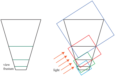
Figure 7.18 On the left, the view frustum from the eye is split into four volumes. On the right, bounding boxes are created for the volumes, which determine the volume rendered by each of the four shadow maps for the directional light. (After Engel [430].)

Figure 7.19 On the left, the scene’s wide viewable area causes a single shadow map at a 2048 × 2048 resolution to exhibit perspective aliasing. On the right, four 1024 × 1024 shadow maps placed along the view axis improve quality considerably [1963]. A zoom of the front corner of the fence is shown in the inset red boxes. (Images courtesy of Fan Zhang, The Chinese University of Hong Kong.)
This type of algorithm is straightforward to implement, can cover huge scene areas with reasonable results, and is robust. The dueling frusta problem can be addressed by sampling at a higher rate closer to the eye, and there are no serious worst-case problems. Because of these strengths, cascaded shadow mapping is used in many applications.
While it is possible to use perspective warping to pack more samples into subdivided areas of a single shadow map [1783], the norm is to use a separate shadow map for each cascade. As Figure 7.18 implies, and Figure 7.20 shows from the viewer’s perspective, the area covered by each map can vary. Smaller view volumes for the closer shadow maps provide more samples where they are needed. Determining how the range of z-depths is split among the maps—a task called z-partitioning—can be quite simple or involved [412, 991, 1791]. One method is logarithmic partitioning [1062], where the ratio of far to near plane distances is made the same for each cascade map:
(7.5)

Figure 7.20 Shadow cascade visualization. Purple, green, yellow, and red represent the nearest through farthest cascades. (Image courtesy of Unity Technologies.)
where n and f are the near and far planes of the whole scene, c is the number of maps, and r is the resulting ratio. For example, if the scene’s closest object is 1 meter away, the maximum distance is 1000 meters, and we have three cascaded maps, then . The near and far plane distances for the closest view would be 1 and 10, the next interval is 10 to 100 to maintain this ratio, and the last is 100 to 1000 meters. The initial near depth has a large effect on this partitioning. If the near depth was only 0.1 meters, then the cube root of 10000 is 21.54, a considerably higher ratio, e.g., 0.1 to 2.154 to 46.42 to 1000. This would mean that each shadow map generated must cover a larger area, lowering its precision. In practice such a partitioning gives considerable resolution to the area close to the near plane, which is wasted if there are no objects in this area. One way to avoid this mismatch is to set the partition distances as a weighted blend of logarithmic and equidistant distributions [1962, 1963], but it would be better still if we could determine tight view bounds for the scene.
The challenge is in setting the near plane. If set too far from the eye, objects may be clipped by this plane, an extremely bad artifact. For a cut scene, an artist can set this value precisely in advance [1590], but for an interactive environment the problem is more challenging. Lauritzen et al. [991, 1403] present sample distribution shadow maps (SDSM), which use the z-depth values from the previous frame to determine a better partitioning by one of two methods.
The first method is to look through the z-depths for the minimum and maximum values and use these to set the near and far planes. This is performed using what is called a reduce operation on the GPU, in which a series of ever-smaller buffers are analyzed by a compute or other shader, with the output buffer fed back as input, until a 1 × 1 buffer is left. Normally, the values are pushed out a bit to adjust for the speed of movement of objects in the scene. Unless corrective action is taken, nearby objects entering from the edge of the screen may still cause problems for a frame, though will quickly be corrected in the next.
The second method also analyzes the depth buffer’s values, making a graph called a histogram that records the distribution of the z-depths along the range. In addition to finding tight near and far planes, the graph may have gaps in it where there are no objects at all. Any partition plane normally added to such an area can be snapped to where objects actually exist, giving more z-depth precision to the set of cascade maps.
In practice, the first method is general, is quick (typically in the 1 ms range per frame), and gives good results, so it has been adopted in several applications [1405, 1811]. See Figure 7.21.

Figure 7.21 Effect of depth bounds. On the left, no special processing is used to adjust the near and far planes. On the right, SDSM is used to find tighter bounds. Note the window frame near the left edge of each image, the area beneath the flower box on the second floor, and the window on the first floor, where undersampling due to loose view bounds causes artifacts. Exponential shadow maps are used to render these particular images, but the idea of improving depth precision is useful for all shadow map techniques. (Image courtesy of Ready at Dawn Studios, copyright Sony Interactive Entertainment.)
As with a single shadow map, shimmering artifacts due to light samples moving frame to frame are a problem, and can be even worse as objects move between cascades. A variety of methods are used to maintain stable sample points in world space, each with their own advantages [41, 865, 1381, 1403, 1678, 1679, 1810]. A sudden change in a shadow’s quality can occur when an object spans the boundary between two shadow maps. One solution is to have the view volumes slightly overlap. Samples taken in these overlap zones gather results from both adjoining shadow maps and are blended [1791]. Alternately, a single sample can be taken in such zone by using dithering [1381].
Due to its popularity, considerable effort has been put into improving efficiency and quality [1791, 1964]. If nothing changes within a shadow map’s frustum, that shadow map does not need to be recomputed. For each light, the list of shadow casters can be precomputed by finding which objects are visible to the light, and of these, which can cast shadows on receivers [1405]. Since it is fairly difficult to perceive whether a shadow is correct, some shortcuts can be taken that are applicable to cascades and other algorithms. One technique is to use a low level of detail model as a proxy to actually cast the shadow [652, 1812]. Another is to remove tiny occluders from consideration [1381, 1811]. The more distant shadow maps may be updated less frequently than once a frame, on the theory that such shadows are less important. This idea risks artifacts caused by large moving objects, so needs to be used with care [865, 1389, 1391, 1678, 1679]. Day [329] presents the idea of “scrolling” distant maps from frame to frame, the idea being that most of each static shadow map is reusable frame to frame, and only the fringes may change and so need rendering. Games such as DOOM (2016) maintain a large atlas of shadow maps, regenerating only those where objects have moved [294]. The farther cascaded maps could be set to ignore dynamic objects entirely, since such shadows may contribute little to the scene. With some environments, a high-resolution static shadow map can be used in place of these farther cascades, which can significantly reduce the workload [415, 1590]. A sparse texture system (Section 19.10.1) can be employed for worlds where a single static shadow map would be enormous [241, 625, 1253]. Cascaded shadow mapping can be combined with baked-in light-map textures or other shadow techniques that are more appropriate for particular situations [652]. Valient’s presentation [1811] is noteworthy in that it describes different shadow system customizations and techniques for a wide range of video games. Section 11.5.1 discusses precomputed light and shadow algorithms in detail.
Creating several separate shadow maps means a run through some set of geometry for each. A number of approaches to improve efficiency have been built on the idea of rendering occluders to a set of shadow maps in a single pass. The geometry shader can be used to replicate object data and send it to multiple views [41]. Instanced geometry shaders allow an object to be output into up to 32 depth textures [1456].
Multiple-viewport extensions can perform operations such as rendering an object to a specific texture array slice [41, 154, 530]. Section 21.3.1 discusses these in more detail, in the context of their use for virtual reality. A possible drawback of viewport-sharing techniques is that the occluders for all the shadow maps generated must be sent down the pipeline, versus the set found to be relevant to each shadow map [1791, 1810].
You yourself are currently in the shadows of billions of light sources around the world. Light reaches you from only a few of these. In real-time rendering, large scenes with multiple lights can become swamped with computation if all lights are active at all times. If a volume of space is inside the view frustum but not visible to the eye, objects that occlude this receiver volume do not need to be evaluated [625, 1137]. Bittner et al. [152] use occlusion culling (Section 19.7) from the eye to find all visible shadow receivers, and then render all potential shadow receivers to a stencil buffer mask from the light’s point of view. This mask encodes which visible shadow receivers are seen from the light. To generate the shadow map, they render the objects from the light using occlusion culling and use the mask to cull objects where no receivers are located. Various culling strategies can also work for lights. Since irradiance falls off with the square of the distance, a common technique is to cull light sources after a certain threshold distance. For example, the portal culling technique in Section 19.5 can find which lights affect which cells. This is an active area of research, since the performance benefits can be considerable [1330, 1604].
7.5 Percentage-Closer Filtering
A simple extension of the shadow-map technique can provide pseudo-soft shadows. This method can also help ameliorate resolution problems that cause shadows to look blocky when a single light-sample cell covers many screen pixels. The solution is similar to texture magnification (Section 6.2.1). Instead of a single sample being taken off the shadow map, the four nearest samples are retrieved. The technique does not interpolate between the depths themselves, but rather the results of their comparisons with the surface’s depth. That is, the surface’s depth is compared separately to the four texel depths, and the point is then determined to be in light or shadow for each shadow-map sample. These results, i.e., 0 for shadow and 1 for light, are then bilinearly interpolated to calculate how much the light actually contributes to the surface location. This filtering results in an artificially soft shadow. These penumbrae change, depending on the shadow map’s resolution, camera location, and other factors. For example, a higher resolution makes for a narrower softening of the edges. Still, a little penumbra and smoothing is better than none at all.
This idea of retrieving multiple samples from a shadow map and blending the results is called percentage-closer filtering (PCF) [1475]. Area lights produce soft shadows. The amount of light reaching a location on a surface is a function of what proportion of the light’s area is visible from the location. PCF attempts to approximate a soft shadow for a punctual (or directional) light by reversing the process.
Instead of finding the light’s visible area from a surface location, it finds the visibility of the punctual light from a set of surface locations near the original location. See Figure 7.22. The name “percentage-closer filtering” refers to the ultimate goal, to find the percentage of the samples taken that are visible to the light. This percentage is how much light then is used to shade the surface.

Figure 7.22 On the left, the brown lines from the area light source show where penumbrae are formed. For a single point p on the receiver, the amount of illumination received could be computed by testing a set of points on the area light’s surface and finding which are not blocked by any occluders. On the right, a point light does not cast a penumbra. PCF approximates the effect of an area light by reversing the process: At a given location, it samples over a comparable area on the shadow map to derive a percentage of how many samples are illuminated. The red ellipse shows the area sampled on the shadow map. Ideally, the width of this disk is proportional to the distance between the receiver and occluder.
In PCF, locations are generated nearby to a surface location, at about the same depth, but at different texel locations on the shadow map. Each location’s visibility is checked, and these resulting boolean values, lit or unlit, are then blended to get a soft shadow. Note that this process is non-physical: Instead of sampling the light source directly, this process relies on the idea of sampling over the surface itself. The distance to the occluder does not affect the result, so shadows have similar-sized penumbrae. Nonetheless this method provides a reasonable approximation in many situations.
Once the width of the area to be sampled is determined, it is important to sample in a way that avoids aliasing artifacts. There are numerous variations of how to sample and filter nearby shadow-map locations. Variables include how wide of an area to sample, how many samples to use, the sampling pattern, and how to weight the results. With less-capable APIs, the sampling process could be accelerated by a special texture sampling mode similar to bilinear interpolation, which accesses the four neighboring locations. Instead of blending the results, each of the four samples is compared to a given value, and the ratio that passes the test is returned [175]. However, performing nearest neighbor sampling in a regular grid pattern can create noticeable artifacts. Using a joint bilateral filter that blurs the result but respects object edges can improve quality while avoiding shadows leaking onto other surfaces [1343]. See Section 12.1.1 for more on this filtering technique.
DirectX 10 introduced single-instruction bilinear filtering support for PCF, giving a smoother result [53, 412, 1709, 1790]. This offers considerable visual improvement over nearest neighbor sampling, but artifacts from regular sampling remain a problem. One solution to minimize grid patterns is to sample an area using a precomputed Poisson distribution pattern, as illustrated in Figure 7.23. This distribution spreads samples out so that they are neither near each other nor in a regular pattern. It is well known that using the same sampling locations for each pixel, regardless of the distribution, can result in patterns [288]. Such artifacts can be avoided by randomly rotating the sample distribution around its center, which turns aliasing into noise. Castan˜o [235] found that the noise produced by Poisson sampling was particularly noticeable for their smooth, stylized content. He presents an efficient Gaussian-weighted sampling scheme based on bilinear sampling.

Figure 7.23 The far left shows PCF sampling in a 4×4 grid pattern, using nearest neighbor sampling. The far right shows a 12-tap Poisson sampling pattern on a disk. Using this pattern to sample the shadow map gives the improved result in the middle left, though artifacts are still visible. In the middle right, the sampling pattern is rotated randomly around its center from pixel to pixel. The structured shadow artifacts turn into (much less objectionable) noise. (Images courtesy of John Isidoro, ATI Research, Inc.)
Self-shadowing problems and light leaks, i.e., acne and Peter Panning, can become worse with PCF. Slope scale bias pushes the surface away from the light based purely on its angle to the light, with the assumption that a sample is no more than a texel away on the shadow map. By sampling in a wider area from a single location on a surface, some of the test samples may get blocked by the true surface.
A few different additional bias factors have been invented and used with some success to reduce the risk of self-shadowing. Burley [212] describes the bias cone, where each sample is moved toward the light proportional to its distance from the original sample. Burley recommends a slope of 2.0, along with a small constant bias. See Figure 7.24.

Figure 7.24 Additional shadow bias methods. For PCF, several samples are taken surrounding the original sample location, the center of the five dots. All these samples should be lit. In the left figure, a bias cone is formed and the samples are moved up to it. The cone’s steepness could be increased to pull the samples on the right close enough to be lit, at the risk of increasing light leaks from other samples elsewhere (not shown) that truly are shadowed. In the middle figure, all samples are adjusted to lie on the receiver’s plane. This works well for convex surfaces but can be counterproductive at concavities, as seen on the left side. In the right figure, normal offset bias moves the samples along the surface’s normal direction, proportional to the sine of the angle between the normal and the light. For the center sample, this can be thought of as moving to an imaginary surface above the original surface. This bias not only affects the depth but also changes the texture coordinates used to test the shadow map.
Schu¨ler [1585], Isidoro [804], and Tuft [1790] present techniques based on the observation that the slope of the receiver itself should be used to adjust the depths of the rest of the samples. Of the three, Tuft’s formulation [1790] is most easily applied to cascaded shadow maps. Dou et al. [373] further refine and extend this concept, accounting for how the z-depth varies in a nonlinear fashion. These approaches assume that nearby sample locations are on the same plane formed by the triangle. Referred to as receiver plane depth bias or other similar terms, this technique can be quite precise in many cases, as locations on this imaginary plane are indeed on the surface, or in front of it if the model is convex. As shown in Figure 7.24, samples near concavities can become hidden. Combinations of constant, slope scale, receiver plane, view bias, and normal offset biasing have been used to combat the problem of self-shadowing, though hand-tweaking for each environment can still be necessary [235, 1391, 1403].
One problem with PCF is that because the sampling area’s width remains constant, shadows will appear uniformly soft, all with the same penumbra width. This may be acceptable under some circumstances, but appears incorrect where there is ground contact between the occluder and receiver. See Figure 7.25.

Figure 7.25 Percentage-closer filtering and percentage-closer soft shadows. On the left, hard shadows with a little PCF filtering. In the middle, constant width soft shadows. On the right, variable-width soft shadows with proper hardness where objects are in contact with the ground. (Images courtesy of NVIDIA Corporation.)
7.6 Percentage-Closer Soft Shadows
In 2005 Fernando [212, 467, 1252] published an influential approach called percentagecloser soft shadows (PCSS). It attempts a solution by searching the nearby area on the shadow map to find all possible occluders. The average distance of these occluders from the location is used to determine the sample area width:
(7.6)
where d r is the distance of the receiver from the light and d 0 the average occluder distance. In other words, the width of the surface area to the sample grows as the average occluder gets farther from the receiver and closer to the light. Examine Figure 7.22 and think about the effect of moving the occluder to see how this occurs. Figures 7.2 (page 224), 7.25, and 7.26 show examples.
If there are no occluders found, the location is fully lit and no further processing is necessary. Similarly, if the location is fully occluded, processing can end. Otherwise, then the area of interest is sampled and the light’s approximate contribution is computed. To save on processing costs, the width of the sample area can be used to vary the number of samples taken. Other techniques can be implemented, e.g., using lower sampling rates for distant soft shadows that are less likely to be important.
A drawback of this method is that it needs to sample a fair-sized area of the shadow map to find the occluders. Using a rotated Poisson disk pattern can help hide undersampling artifacts [865, 1590]. Jimenez [832] notes that Poisson sampling can be unstable under motion and finds that a spiral pattern formed by using a function halfway between dithering and random gives a better result frame to frame.
Sikachev et al. [1641] discuss in detail a faster implementation of PCSS using features in SM 5.0, introduced by AMD and often called by their name for it, contact hardening shadows (CHS). This new version also addresses another problem with basic PCSS: The penumbra’s size is affected by the shadow map’s resolution. See Figure 7.25. This problem is minimized by first generating mipmaps of the shadow map, then choosing the mip level closest to a user-defined world-space kernel size. An 8 × 8 area is sampled to find the average blocker depth, needing only 16 GatherRed() texture calls. Once a penumbra estimate is found, the higher-resolution mip levels are used for the sharp area of the shadow, while the lower-resolution mip levels are used for softer areas.
CHS has been used in a large number of video games [1351, 1590, 1641, 1678, 1679], and research continues. For example, Buades et al. [206] present separable soft shadow mapping (SSSM), where the PCSS process of sampling a grid is split into separable parts and elements are reused as possible from pixel to pixel.
One concept that has proven helpful for accelerating algorithms that need multiple samples per pixel is the hierarchical min/max shadow map. While shadow map depths normally cannot be averaged, the minimum and maximum values at each mipmap level can be useful. That is, two mipmaps can be formed, one saving the largest zdepth found in each area (sometimes called HiZ), and one the smallest. Given a texel location, depth, and area to be sampled, the mipmaps can be used to rapidly determine fully lit and fully shadowed conditions. For example, if the texel’s z-depth is greater than the maximum z-depth stored for the corresponding area of the mipmap, then the texel must be in shadow—no further samples are needed. This type of shadow map makes the task of determining light visibility much more efficient [357, 415, 610, 680, 1064, 1811].
Methods such as PCF work by sampling the nearby receiver locations. PCSS works by finding an average depth of nearby occluders. These algorithms do not directly take into account the area of the light source, but rather sample the nearby surfaces, and are affected by the resolution of the shadow map. A major assumption behind PCSS is that the average blocker is a reasonable estimate of the penumbra size. When two occluders, say a street lamp and a distant mountain, partially occlude the same surface at a pixel, this assumption is broken and can lead to artifacts. Ideally, we want to determine how much of the area light source is visible from a single receiver location. Several researchers have explored backprojection using the GPU. The idea is to treat each receiver’s location as a viewpoint and the area light source as part of a view plane, and to project occluders onto this plane. Both Schwarz and Stamminger [1593] and Guennebaud et al. [617] summarize previous work and offer their own improvements. Bavoil et al. [116] take a different approach, using depth peeling to create a multi-layer shadow map. Backprojection algorithms can give excellent results, but the high cost per pixel has (so far) meant they have not seen adoption in interactive applications.
7.7 Filtered Shadow Maps
One algorithm that allows filtering of the shadow maps generated is Donnelly and Lauritzen’s variance shadow map (VSM) [368]. The algorithm stores the depth in one map and the depth squared in another map. MSAA or other antialiasing schemes can be used when generating the maps. These maps can be blurred, mipmapped, put in summed area tables [988], or any other method. The ability to treat these maps as filterable textures is a huge advantage, as the entire array of sampling and filtering techniques can be brought to bear when retrieving data from them.
We will describe VSM in some depth here, to give a sense of how this process works; also, the same type of testing is used for all methods in this class of algorithm. Readers interested in learning more about this area should access the relevant references, and we also recommend the book by Eisemann et al. [412], which gives the topic considerably more space.
To begin, for VSM the depth map is sampled (just once) at the receiver’s location to return an average depth of the closest light occluder. When this average depth M 1, called the first moment, is greater than the depth on the shadow receiver t, the receiver is considered fully in light. When the average depth is less than the receiver’s depth, the following equation is used:
(7.7)
where p max is the maximum percentage of samples in light, σ 2 is the variance, t is the receiver depth, and M 1 is the average expected depth in the shadow map. The depthsquared shadow map’s sample M 2, called the second moment, is used to compute the variance:
(7.8)
The value p max is an upper bound on the visibility percentage of the receiver. The actual illumination percentage p cannot be larger than this value. This upper bound is from the one-sided variant of Chebyshev’s inequality. The equation attempts to estimate, using probability theory, how much of the distribution of occluders at the surface location is beyond the surface’s distance from the light. Donnelly and Lauritzen show that for a planar occluder and planar receiver at fixed depths, p= p max, so Equation 7.7 can be used as a good approximation of many real shadowing situations.
Myers [1251] builds up an intuition as to why this method works. The variance over an area increases at shadow edges. The greater the difference in depths, the greater the variance. The (t− M 1)2 term is then a significant determinant in the visibility percentage. If this value is just slightly above zero, this means the average occluder depth is slightly closer to the light than the receiver, and p max is then near 1 (fully lit). This would happen along the fully lit edge of the penumbra. Moving into the penumbra, the average occluder depth gets closer to the light, so this term becomes larger and p max drops. At the same time the variance itself is changing within the penumbra, going from nearly zero along the edges to the largest variance where the occluders differ in depth and equally share the area. These terms balance out to give a linearly varying shadow across the penumbra. See Figure 7.26 for a comparison with other algorithms.

Figure 7.26 In the upper left, standard shadow mapping. Upper right, perspective shadow mapping, increasing the density of shadow-map texel density near the viewer. Lower left, percentage-closer soft shadows, softening the shadows as the occluder’s distance from the receiver increases. Lower right, variance shadow mapping with a constant soft shadow width, each pixel shaded with a single variance map sample. (Images courtesy of Nico Hempe, Yvonne Jung, and Johannes Behr.)
One significant feature of variance shadow mapping is that it can deal with the problem of surface bias problems due to geometry in an elegant fashion. Lauritzen [988] gives a derivation of how the surface’s slope is used to modify the value of the second moment. Bias and other problems from numerical stability can be a problem for variance mapping. For example, Equation 7.8 subtracts one large value from another similar value. This type of computation tends to magnify the lack of accuracy of the underlying numerical representation. Using floating point textures helps avoid this problem.
Overall VSM gives a noticeable increase in quality for the amount of time spent processing, since the GPU’s optimized texture capabilities are used efficiently. While PCF needs more samples, and hence more time, to avoid noise when generating softer shadows, VSM can work with just a single, high-quality sample to determine the entire area’s effect and produce a smooth penumbra. This ability means that shadows can be made arbitrarily soft at no additional cost, within the limitations of the algorithm.
As with PCF, the width of the filtering kernel determines the width of the penumbra. By finding the distance between the receiver and the closest occluder, the kernel width can be varied, so giving convincing soft shadows. Mipmapped samples are poor estimators of coverage for a penumbra with a slowly increasing width, creating boxy artifacts. Lauritzen [988] details how to use summed-area tables to give considerably better shadows. An example is shown in Figure 7.27.

Figure 7.27 Variance shadow mapping, where the distance to the light source increases from left to right. (Images from the NVIDIA SDK 10 [1300] samples, courtesy of NVIDIA Corporation.)
One place variance shadow mapping breaks down is along the penumbrae areas when two or more occluders cover a receiver and one occluder is close to the receiver. The Chebyshev inequality from probability theory will produce a maximum light value that is not related to the correct light percentage. The closest occluder, by only partially hiding the light, throws off the equation’s approximation. This results in light bleeding (a.k.a. light leaks), where areas that are fully occluded still receive light. See Figure 7.28. By taking more samples over smaller areas, this problem can be resolved, turning variance shadow mapping into a form of PCF. As with PCF, speed and performance trade off, but for scenes with low shadow depth complexity, variance mapping works well. Lauritzen [988] gives one artist-controlled method to ameliorate the problem, which is to treat low percentages as fully shadowed and to remap the rest of the percentage range to 0% to 100%. This approach darkens light bleeds, at the cost of narrowing penumbrae overall. While light bleeding is a serious limitation, VSM is good for producing shadows from terrain, since such shadows rarely involve multiple occluders [1227].

Figure 7.28 On the left, variance shadow mapping applied to a teapot. On the right, a triangle (not shown) casts a shadow on the teapot, causing objectionable artifacts in the shadow on the ground. (Images courtesy of Marco Salvi.)
The promise of being able to use filtering techniques to rapidly produce smooth shadows generated much interest in filtered shadow mapping; the main challenge is solving the various bleeding problems. Annen et al. [55] introduced the convolution shadow map. Extending the idea behind Soler and Sillion’s algorithm for planar receivers [1673], the idea is to encode the shadow depth in a Fourier expansion. As with variance shadow mapping, such maps can be filtered. The method converges to the correct answer, so the light leak problem is lessened.
A drawback of convolution shadow mapping is that several terms need to be computed and accessed, considerably increasing both execution and storage costs [56, 117]. Salvi [1529, 1530] and Annen et al. [56] concurrently and independently came upon the idea of using a single term based on an exponential function. Called an exponential shadow map (ESM) or exponential variance shadow map (EVSM), this method saves the exponential of the depth along with its second moment into two buffers. An exponential function more closely approximates the step function that a shadow map performs (i.e., in light or not), so this works to significantly reduce bleeding artifacts. It avoids another problem that convolution shadow mapping has, called ringing, where minor light leaks can happen at particular depths just past the original occluder’s depth.
A limitation with storing exponential values is that the second moment values can become extremely large and so run out of range using floating point numbers. To improve precision, and to allow the exponential function to drop off more steeply, z-depths can be generated so that they are linear [117, 258].
Due to its improved quality over VSM, and its lower storage and better performance compared to convolution maps, the exponential shadow map approach has sparked the most interest of the three filtered approaches. Pettineo [1405] notes several other improvements, such as the ability to use MSAA to improve results and to obtain some limited transparency, and describes how filtering performance can be improved with compute shaders.
More recently, moment shadow mapping was introduced by Peters and Klein [1398]. It offers better quality, though at the expense of using four or more moments, increasing storage costs. This cost can be decreased by the use of 16-bit integers to store the moments. Pettineo [1404] implements and compares this new approach with ESM, providing a code base that explores many variants.
Cascaded shadow-map techniques can be applied to filtered maps to improve precision [989]. An advantage of cascaded ESM over standard cascaded maps is that a single bias factor can be set for all cascades [1405]. Chen and Tatarchuk [258] go into detail about various light leak problems and other artifacts encountered with cascaded ESM, and present a few solutions.
Filtered maps can be thought of as an inexpensive form of PCF, one that needs few samples. Like PCF, such shadows have a constant width. These filtered approaches can all be used in conjunction with PCSS to provide variable-width penumbrae [57, 1620, 1943]. An extension of moment shadow mapping also includes the ability to provide light scattering and transparency effects [1399].
7.8 Volumetric Shadow Techniques
Transparent objects will attenuate and change the color of light. For some sets of transparent objects, techniques similar to those discussed in Section 5.5 can be used to simulate such effects. For example, in some situations a second type of shadow map can be generated. The transparent objects are rendered to it, and the closest depth and color or alpha coverage is stored. If the receiver is not blocked by the opaque shadow map, the transparency depth map is then tested and, if occluded, the color or coverage is retrieved as needed [471, 1678, 1679]. This idea is reminiscent of shadow and light projection in Section 7.2, with the stored depths avoiding projection onto receivers between the transparent objects and the light. Such techniques cannot be applied to the transparent objects themselves.
Self-shadowing is critical for realistic rendering of objects such as hair and clouds, where objects are either small or semitransparent. Single-depth shadow maps will not work for these situations. Lokovic and Veach [1066] first presented the concept of deep shadow maps, in which each shadow-map texel stores a function of how light drops off with depth. This function is typically approximated by a series of samples at different depths, with each sample having an opacity value. The two samples in the map that bracket a given position’s depth are used to find the shadow’s effect. The challenge on the GPU is in generating and evaluating such functions efficiently. These algorithms use similar approaches and run into similar challenges found for some order-independent transparency algorithms (Section 5.5), such as compact storage of the data needed to faithfully represent each function.
Kim and Neumann [894] were the first to present a GPU-based method, which they call opacity shadow maps. Maps storing just the opacities are generated at a fixed set of depths. Nguyen and Donnelly [1274] give an updated version of this approach, producing images such as Figure 17.2 on page 719. However, the depth slices are all parallel and uniform, so many slices are needed to hide in-between slice opacity artifacts due to linear interpolation. Yuksel and Keyser [1953] improve efficiency and quality by creating opacity maps that more closely follow the shape of the model.
Doing so allows them to reduce the number of layers needed, as evaluation of each layer is more significant to the final image.
To avoid having to rely on fixed slice setups, more adaptive techniques have been proposed. Salvi et al. [1531] introduce adaptive volumetric shadow maps, in which each shadow-map texel stores both the opacities and layer depths. Pixel shaders operations are used to lossily compress the stream of data (surface opacities) as it is rasterized. This avoids needing an unbounded amount of memory to gather all samples and process them in a set. The technique is similar to deep shadow maps [1066], but with the compression step done on the fly in the pixel shader. Limiting the function representation to a small, fixed number of stored opacity/depth pairs makes both compression and retrieval on the GPU more efficient [1531]. The cost is higher than simple blending because the curve needs to be read, updated, and written back, and it depends on the number of points used to represent a curve. In this case, this technique also requires recent hardware that supports UAV and ROV functionality (end of Section 3.8). See Figure 7.29 for an example.

Figure 7.29 Hair and smoke rendering with adaptive volumetric shadow maps [1531]. (Reprinted by permission of Marco Salvi and Intel Corporation, copyright Intel Corporation, 2010.)
The adaptive volumetric shadow mapping method was used for realistic smoke rendering in the game GRID2, with the average cost being below 2 ms/frame [886]. Fu¨rst et al. [509] describe and provide code for their implementation of deep shadow maps for a video game. They use linked lists to store depths and alphas, and use exponential shadow mapping to provide a soft transition between lit and shadowed regions.
Exploration of shadow algorithms continues, with a synthesis of a variety of algorithms and techniques becoming more common. For example, Selgrad et al. [1603] research storing multiple transparent samples with linked lists and using compute shaders with scattered writes to build the map. Their work uses deep shadow-map concepts, along with filtered maps and other elements, which give a more general solution for providing high-quality soft shadows.
7.9 Irregular Z-Buffer Shadows
Shadow-map approaches of various sorts are popular for several reasons. Their costs are predictable and scale well to increasing scene sizes, at worst linear with the number of primitives. They map nicely onto the GPU, as they rely on rasterization to regularly sample the light’s view of the world. However, due to this discrete sampling, problems arise because the locations the eye sees do not map one-to-one with those the light sees. Various aliasing problems arise when the light samples a surface less frequently than the eye. Even when sampling rates are comparable, there are biasing problems because the surface is sampled in locations slightly different than those the eye sees.
Shadow volumes provide an exact, analytical solution, as the light’s interactions with surfaces result in sets of triangles defining whether any given location is lit or in shadow. The unpredictable cost of the algorithm when implemented on the GPU is a serious drawback. The improvements explored in recent years [1648] are tantalizing, but have not yet had an “existence proof” of being adopted in commercial applications. Another analytical shadow-testing method may have potential in the longer term: ray tracing. Described in detail in Section 11.2.2, the basic idea is simple enough, especially for shadowing. A ray is shot from the receiver location to the light. If any object is found that blocks the ray, the receiver is in shadow. Much of a fast ray tracer’s code is dedicated to generating and using hierarchical data structures to minimize the number of object tests needed per ray. Building and updating these structures each frame for a dynamic scene is a decades-old topic and a continuing area of research.
Another approach is to use the GPU’s rasterization hardware to view the scene, but instead of just z-depths, additional information is stored about the edges of the occluders in each grid cell of the light [1003, 1607]. For example, imagine storing at each shadow-map texel a list of triangles that overlap the grid cell. Such a list can be generated by conservative rasterization, in which a triangle generates a fragment if any part of the triangle overlaps a pixel, not just the pixel’s center (Section 23.1.2). One problem with such schemes is that the amount of data per texel normally needs to be limited, which in turn can lead to inaccuracies in determining the status of every receiver location. Given modern linked-list principles for GPUs [1943], it is certainly possible to store more data per pixel. However, aside from physical memory limits, a problem with storing a variable amount of data in a list per texel is that GPU processing can become extremely inefficient, as a single warp can have a few fragment threads that need to retrieve and process many items, while the rest of the threads are idle, having no work to do. Structuring a shader to avoid thread divergence due to dynamic “if” statements and loops is critical for performance.
An alternative to storing triangles or other data in the shadow map and testing receiver locations against them is to flip the problem, storing receiver locations and then testing triangles against each. This concept of saving the receiver locations, first explored by Johnson et al. [839] and Aila and Laine [14], is called the irregular z-buffer (IZB). The name is slightly misleading, in that the buffer itself has a normal, regular shape for a shadow map. Rather, the buffer’s contents are irregular, as each shadowmap texel will have one or more receiver locations stored in it, or possibly none at all. See Figure 7.30.

Figure 7.30 Irregular z-buffer. In the upper left, the view from the eye generates a set of dots at the pixel centers. Two triangles forming a cube face are shown. In the upper right, these dots are shown from the light’s view. In the lower left, a shadow-map grid is imposed. For each texel a list of all dots inside its grid cell is generated. In the lower right, shadow testing is performed for the red triangle by conservatively rasterizing it. At each texel touched, shown in light red, all dots in its list are tested against the triangle for visibility by the light. (Underlying raster images courtesy of Timo Aila and Samuli Laine [14].)
Using the method presented by Sintorn et al. [1645] and Wyman et al. [1930, 1932], a multi-pass algorithm creates the IZB and tests its contents for visibility from the light. First, the scene is rendered from the eye, to find the z-depths of the surfaces seen from the eye. These points are transformed to the light’s view of the scene, and tight bounds are formed from this set for the light’s frustum. The points are then deposited in the light’s IZB, each placed into a list at its corresponding texel. Note that some lists may be empty, a volume of space that the light views but that has no surfaces seen by the eye. Occluders are conservatively rasterized to the light’s IZB to determine whether any points are hidden, and so in shadow. Conservative rasterization ensures that, even if a triangle does not cover the center of a light texel, it will be tested against points it may overlap nonetheless.
Visibility testing occurs in the pixel shader. The test itself can be visualized as a form of ray tracing. A ray is generated from an image point’s location to the light. If a point is inside the triangle and more distant than the triangle’s plane, it is hidden. Once all occluders are rasterized, the light-visibility results are used to shade the surface. This testing is also called frustum tracing, as the triangle can be thought of as defining a view frustum that checks points for inclusion in its volume.
Careful coding is critical in making this approach work well with the GPU. Wyman et al. [1930, 1932] note that their final version was two orders of magnitude faster than the initial prototypes. Part of this performance increase was straightforward algorithm improvements, such as culling image points where the surface normal was facing away from the light (and so always unlit) and avoiding having fragments generated for empty texels. Other performance gains were from improving data structures for the GPU, and from minimizing thread divergence by working to have short, similar-length lists of points in each texel. Figure 7.30 shows a low-resolution shadow map with long lists for illustrative purposes. The ideal is one image point per list. A higher resolution gives shorter lists, but also increases the number of fragments generated by occluders for evaluation.
As can be seen in the lower left image in Figure 7.30, the density of visible points on the ground plane is considerably higher on the left side than the right, due to the perspective effect. Using cascaded shadow maps helps lower list sizes in these areas by focusing more light-map resolution closer to the eye.
This approach avoids the sampling and bias issues of other approaches and provides perfectly sharp shadows. For aesthetic and perceptual reasons, soft shadows are often desired, but can have bias problems with nearby occluders, such as Peter Panning. Story and Wyman [1711, 1712] explore hybrid shadow techniques. The core idea is to use the occluder distance to blend IZB and PCSS shadows, using the hard shadow result when the occluder is close and soft when more distant. See Figure 7.31. Shadow quality is often most important for nearby objects, so IZB costs can be reduced by using this technique on only a selected subset. This solution has successfully been used in video games. This chapter started with such an image, shown in Figure 7.2 on page 224.
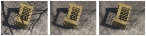
Figure 7.31 On the left, PCF gives uniformly softened shadows for all objects. In the middle, PCSS softens the shadow with distance to the occluder, but the tree branch shadow overlapping the left corner of the crate creates artifacts. On the right, sharp shadows from IZB blended with soft from PCSS give an improved result [1711]. (Images from “Tom Clancy’s The Division,” courtesy of Ubisoft.)
7.10 Other Applications
Treating the shadow map as defining a volume of space, separating light from dark, can also help in determining what parts of objects to shadow. Gollent [555] describes how CD Projekt’s terrain shadowing system computes for each area a maximum height that is still occluded, which can then be used to shadow not only terrain but also trees and other elements in the scene. To find each height, a shadow map of the visible area is rendered for the sun. Each terrain heightfield location is then checked for visibility from the sun. If in shadow, the height where the sun is first visible is estimated by increasing the world height by a fixed step size until the sun comes into view and then performing a binary search. In other words, we march along a vertical line and iterate to narrow down the location where it intersects the shadow map’s surface that separates light from dark. Neighboring heights are interpolated to find this occlusion height at any location. An example of this technique used for soft shadowing of a terrain heightfield can be seen in Figure 7.32. We will see more use of ray marching through areas of light and dark in Chapter 14.

Figure 7.32 Terrain lit with the height where the sun is first seen computed for each heightfield location. Note how trees along the shadow’s edge are properly shadowed [555]. (CD PROJEKT R, The Witcher R are registered trademarks of CD PROJEKT Capital Group. The Witcher game c CD PROJEKT S.A. Developed by CD PROJEKT S.A. All rights reserved. The Witcher game is based on the prose of Andrzej Sapkowski. All other copyrights and trademarks are the property of their respective owners.)
One last method worth a mention is rendering screen-space shadows. Shadow maps often fail to produce accurate occlusions on small features, because of their limited resolution. This is especially problematic when rendering human faces, because we are particularly prone to noticing any visual artifacts on them. For example, rendering glowing nostrils (when not intended) looks jarring. While using higher-resolution shadow maps or a separate shadow map targeting only the area of interest can help, another possibility is to leverage the already-existing data. In most modern rendering engines the depth buffer from the camera perspective, coming from an earlier prepass, is available during rendering. The data stored in it can be treated as a heightfield. By iteratively sampling this depth buffer, we can perform a ray-marching process (Section 6.8.1) and check if the direction toward the light is unoccluded. While costly, as it involves repeatedly sampling the depth buffer, doing so can provide high-quality results for closeups in cut scenes, where spending extra milliseconds is often justified. The method was proposed by Sousa at al. [1678] and is commonly used in many game engines today [384, 1802].
To summarize this whole chapter, shadow mapping in some form is by far the most common algorithm used for shadows cast onto arbitrary surface shapes. Cascaded shadow maps improve sampling quality when shadows are cast in a large area, such as an outdoor scene. Finding a good maximum distance for the near plane via SDSM can further improve precision. Percentage-closer filtering (PCF) gives some softness to the shadows, percentage-closer soft shadows (PCSS) and its variants give contact hardening, and the irregular z-buffer can provide precise hard shadows. Filtered shadow maps provide rapid soft-shadow computation and work particularly well when the occluder is far from the receiver, as with terrain. Finally, screen-space techniques can be used for additional precision, though at a noticeable cost.
In this chapter, we have focused on key concepts and techniques currently used in applications. Each has its own strengths, and choices depend on world size, composition (static content versus animated), material types (opaque, transparent, hair, or smoke), and number and type of lights (static or dynamic; local or distant; point, spot, or area), as well as factors such as how well the underlying textures can hide any artifacts. GPU capabilities evolve and improve, so we expect to continue seeing new algorithms that map well to the hardware appear in the years ahead. For example, the sparse-texture technique described in Section 19.10.1 has been applied to shadowmap storage to improve resolution [241, 625, 1253]. In an inventive approach, Sintorn, K¨ampe, and others [850, 1647] explore the idea of converting a two-dimensional shadow map for a light into a three-dimensional set of voxels (small boxes; see Section 13.10). An advantage of using a voxel is that it can be categorized as lit or in shadow, thus needing minimal storage. A highly compressed sparse voxel octree representation stores shadows for a huge number of lights and static occluders. Scandolo et al. [1546] combine their compression technique with an interval-based scheme using dual shadow maps, giving still higher compression rates. Kasyan [865] uses voxel cone tracing (Section 13.10) to generate soft shadows from area lights. See Figure 7.33 for an example. More cone-traced shadows are shown in Figure 13.33 on page 585.

Figure 7.33 At the top is an image generated with a basic soft-shadows approximation. At the bottom is voxel-based area light shadowing using cone tracing, on a voxelization of the scene. Note the considerably more diffuse shadows for the cars. Lighting also differs due to a change in the time of day. (Images courtesy of Crytek [865].)
Further Reading and Resources
Our focus in this chapter is on basic principles and what qualities a shadow algorithm needs—predictable quality and performance—to be useful for interactive rendering. We have avoiding an exhaustive categorization of the research done in this area of rendering, as two texts tackle the subject. The book Real-Time Shadows by Eisemann et al. [412] focuses directly on interactive rendering techniques, discussing a wide range of algorithms along with their strengths and costs. A SIGGRAPH 2012 course provides an excerpt of this book, while also adding references to newer work [413]. Presentations from their SIGGRAPH 2013 course are available at their website, www. realtimeshadows.com. Woo and Poulin’s book Shadow Algorithms Data Miner [1902] provides an overview of a wide range of shadow algorithms for interactive and batch rendering. Both books supply references to hundreds of research articles in the field. Tuft’s pair of articles [1791, 1792] are an excellent overview of commonly used shadow-mapping techniques and the issues involved. Bjørge [154] presents a range of popular shadow algorithms suitable for mobile devices, along with images comparing various algorithms. Lilley’s presentation [1046] gives a solid and extensive overview of practical shadow algorithms, with a focus on terrain rendering for GIS systems. Blog articles by Pettineo [1403, 1404] and Castan˜o [235] are particularly valuable for their practical tips and solutions, as well as a demo code base. See Scherzer et al. [1558] for a shorter summary of work specifically focused on hard shadows. The survey of algorithms for soft shadows by Hasenfratz et al. [675] is dated, but covers a wide range of early work in some depth.