
Chapter 19
Acceleration Algorithms
“Now here, you see, it takes all the running you can do to keep in the same place. If you want to get somewhere else, you must run at least twice as fast as that!”
—Lewis Carroll
One of the great myths concerning computers is that one day we will have enough processing power. Even in a relatively simple application such as word processing, we find that additional power can be applied to all sorts of features, such as on-the-fly spell and grammar checking, antialiased text display, and dictation.
In real-time rendering, we have at least four performance goals: more frames per second, higher resolution and sampling rates, more realistic materials and lighting, and increased geometrical complexity. A speed of 60–90 frames per second is generally considered fast enough. Even with motion blurring, which can lower the frame rate needed for image quality, a fast rate is still needed to minimize latency when interacting with a scene [1849].
Today, we have 4k displays with resolution; 8k displays with resolution exist, but are not common yet. A 4k display typically has around 140–150 dots per inch (DPI), sometimes called pixels per inch (PPI). Mobile phone displays have values ranging on up to around 400 DPI. A resolution of 1200 DPI, 64 times the number of pixels of a 4k display, is offered by many printer companies today. Even with a limit on screen resolution, antialiasing increases the number of samples needed for generating high-quality images. As discussed in Section 23.6, the number of bits per color channel can also be increased, which drives the need for higher-precision (and therefore more costly) computations.
As previous chapters have shown, describing and evaluating an object’s material can be computationally complex. Modeling the interplay of light and surface can soak up an arbitrarily high amount of computing power. This is true because an image should ultimately be formed by the contributions of light traveling down a limitless number of paths from an illumination source to the eye.
Frame rate, resolution, and shading can always be made more complex, but there is some sense of diminishing returns to increasing any of these. However, there is no real upper limit on scene complexity. The rendering of a Boeing 777 includes 132,500 unique parts and over 3,000,000 fasteners, which yields a polygonal model with over 500,000,000 polygons [310]. See Figure 19.1. Even if most of those objects are not seen due to their small size or position, some work must be done to determine that this is the case. Neither z-buffering nor ray tracing can handle such models without the use of techniques to reduce the sheer number of computations needed. Our conclusion: Acceleration algorithms will always be needed.

Figure 19.1. A “reduced” Boeing model with a mere 350 million triangles rendered with ray tracing. Sectioning is performed by using a user-defined clipping plane. (Image courtesy of Computer Graphics Group, Saarland University. Source 3D data provided by and used with permission of the Boeing Company.)
In this chapter we offer a smörgåsbord of algorithms for accelerating computer graphics rendering, in particular the rendering of large amounts of geometry. The core of many such algorithms is based on spatial data structures, which are described in the next section. Based on that knowledge, we then continue with culling techniques. These are algorithms that try to rapidly determine which objects are visible and need to be treated further. Level of detail techniques reduce the complexity of rendering the remaining objects. To close the chapter, we discuss systems for rendering huge models, including virtual texturing, streaming, transcoding, and terrain rendering.
19.1 Spatial Data Structures
A spatial data structure is one that organizes geometry in some n-dimensional space. Only two- and three-dimensional structures are used in this book, but the concepts can often easily be extended to higher dimensions. These data structures can be used to accelerate queries about whether geometric entities overlap. Such queries are used in a wide variety of operations, such as culling algorithms, during intersection testing and ray tracing, and for collision detection.
The organization of spatial data structures is usually hierarchical. This means, loosely speaking, that the topmost level contains some children, each defining its own volume of space and which in turn contains its own children. Thus, the structure is nested and of a recursive nature. Geometry is referenced by some of the elements in this hierarchy. The main reason for using a hierarchy is that different types of queries get significantly faster, typically an improvement from O(n) to . That is, instead of searching through all n objects, we visit a small subset when performing operations such as finding the closest object in a given direction. Construction time of a spatial data structure can be expensive, and depends on both the amount of geometry inside it and the desired quality of the data structure. However, major advances in this field have reduced construction times considerably, and in some situations it can be done in real time. With lazy evaluation and incremental updates, the construction time can be reduced further still.
Some common types of spatial data structures are bounding volume hierarchies, variants of binary space partitioning (BSP) trees, quadtrees, and octrees. BSP trees and octrees are data structures based on space subdivision. This means that the entire space of the scene is subdivided and encoded in the data structure. For example, the union of the space of all the leaf nodes is equal to the entire space of the scene. Normally the leaf nodes’ volumes do not overlap, with the exception of less common structures such as loose octrees. Most variants of BSP trees are irregular, which means that the space can be subdivided more arbitrarily. The octree is regular, meaning that space is split in a uniform fashion. Though more restrictive, this uniformity can often be a source of efficiency. A bounding volume hierarchy, on the other hand, is not a space subdivision structure. Rather, it encloses the regions of the space surrounding geometrical objects, and thus the BVH need not enclose all space at each level.
BVHs, BSP trees, and octrees are all described in the following sections, along with the scene graph, which is a data structure more concerned with model relationships than with efficient rendering.
19.1.1. Bounding Volume Hierarchies
A bounding volume (BV) is a volume that encloses a set of objects. The idea of a BV is that it should be a much simpler geometrical shape than the contained objects, so that tests using a BV can be done much faster than using the objects themselves. Examples of BVs are spheres, axis-aligned bounding boxes (AABBs), oriented bounding boxes (OBBs), and k-DOPs. See Section for definitions. A BV does not contribute visually to the rendered image. Instead, it is used as a proxy in place of the bounded objects, to speed up rendering, selection, queries, and other computations.
For real-time rendering of three-dimensional scenes, the bounding volume hierarchy is often used for hierarchical view frustum culling (Section 19.4). The scene is organized in a hierarchical tree structure, consisting of a set of connected nodes. The topmost node is the root, which has no parents. An internal node has pointers to its children, which are other nodes. The root is thus an internal node, unless it is the only node in the tree. A leaf node holds the actual geometry to be rendered, and it does not have any children nodes. Each node, including leaf nodes, in the tree has a bounding volume that encloses the geometry in its entire subtree. One may also decide to exclude BVs from the leaf nodes, and instead include them in an internal node just above each leaf node. This setup is where the name bounding volume hierarchy stems from. Each node’s BV encloses the geometry of all the leaf nodes in its subtree. This means that the root has a BV that contains the entire scene. An example of a BVH is shown in Figure 19.2. Note that some of the larger bounding circles could be made tighter, as each node needs to contain only the geometry in its subtree, not the BVs of the descendant nodes. For bounding circles (or spheres), forming such tighter nodes can be expensive, as all geometry in its subtree would have to be examined by each node. In practice, a node’s BV is often formed “bottom up” through the tree, by making a BV that contains the BVs of its children.

Figure 19.2. The left part shows a simple scene with five objects, with bounding circles that are used in the bounding volume hierarchy to the right. A single circle encloses all objects, and then smaller circles are inside the large circle, in a recursive manner. The right part shows the bounding volume hierarchy (tree) that is used to represent the object hierarchy on the left.
The underlying structure of a BVH is a tree, and in the field of computer science the literature on tree data structures is vast. Here, only a few important results will be mentioned. For more information, see, for example, the book Introduction to Algorithms by Cormen et al. [292].
Consider a k-ary tree, that is, a tree where each internal node has k children. A tree with only one node (the root) is said to be of height 0. A leaf node of the root is at height 1, and so on. A balanced tree is a tree in which all leaf nodes either are at height h or . In general, the height, h, of a balanced tree is , where n is the total number of nodes (internal and leaves) in the tree. Note that a higher k gives a tree with a lower height, which means that it takes fewer steps to traverse the tree, but it also requires more work at each node. The binary tree is often the simplest choice, and one that gives reasonable performance. However, there is evidence that a higher k (e.g., or ) gives better performance for some applications [980,1829]. Using , , or makes it simple to construct trees; just subdivide along the longest axis for , and for the two longest axes for , and for all axes for . It is more difficult to form good trees for other values of k. Trees with a higher number, e.g., , of children per node are often preferred from a performance perspective, since they reduce average tree depth and the number of indirections (pointers from parent to child) to follow.
BVHs are excellent for performing various queries. For example, assume that a ray should be intersected with a scene, and the first intersection found should be returned, as would be the case for a shadow ray. To use a BVH for this, testing starts at the root. If the ray misses its BV, then the ray misses all geometry contained in the BVH. Otherwise, testing continues recursively, that is, the BVs of the children of the root are tested. As soon as a BV is missed by the ray, testing can terminate on that subtree of the BVH. If the ray hits a leaf node’s BV, the ray is tested against the geometry at this node. The performance gains come partly from the fact that testing the ray with the BV is fast. This is why simple objects such as spheres and boxes are used as BVs. The other reason is the nesting of BVs, which allows us to avoid testing large regions of space due to early termination in the tree.
Often the closest intersection, not the first found, is what is desired. The only additional data needed are the distance and identity of the closest object found while traversing the tree. The current closest distance is also used to cull the tree during traversal. If a BV is intersected, but its distance is beyond the closest distance found so far, then the BV can be discarded. When examining a parent box, we intersect all children BVs and find the closest. If an intersection is found in this BV’s descendants, this new closest distance is used to cull out whether the other children need to be traversed. As will be seen, a BSP tree has an advantage over normal BVHs in that it can guarantee front-to-back ordering, versus this rough sort that BVHs provide.
BVHs can be used for dynamic scenes as well [1465]. When an object contained in a BV has moved, simply check whether it is still contained in its parent’s BV. If it is, then the BVH is still valid. Otherwise, the object node is removed and the parent’s BV recomputed. The node is then recursively inserted back into the tree from the root. Another method is to grow the parent’s BV to hold the child recursively up the tree as needed. With either method, the tree can become unbalanced and inefficient as more and more edits are performed. Another approach is to put a BV around the limits of movement of the object over some period of time. This is called a temporal bounding volume [13]. For example, a pendulum could have a bounding box that enclosed the entire volume swept out by its motion. One can also perform a bottom-up refit [136] or select parts of the tree to refit or rebuild [928,981,1950].
To create a BVH, one must first be able to compute a tight BV around a set of objects. This topic is treated in Section 22.3. Then, the actual hierarchy of BVs must be created.
19.1.2. BSP Trees
Binary space partitioning trees, or BSP trees for short, exist as two noticeably different variants in computer graphics, which we call axis-aligned and polygon-aligned. The trees are created by using a plane to divide the space in two, and then sorting the geometry into these two spaces. This division is done recursively. One worthwhile property is that if a BSP tree is traversed in a certain way, the geometrical contents of the tree can be sorted front to back from any point of view. This sorting is approximate for axis-aligned and exact for polygon-aligned BSPs. Note that the axis-aligned BSP tree is also called a k-d tree
Axis-Aligned BSP Trees (k-D Trees)
An axis-aligned BSP tree is created as follows. First, the whole scene is enclosed in an axis-aligned bounding box (AABB). The idea is then to recursively subdivide this box into smaller boxes. Now, consider a box at any recursion level. One axis of the box is chosen, and a perpendicular plane is generated that divides the space into two boxes. Some schemes fix this partitioning plane so that it divides the box exactly in half; others allow the plane to vary in position. With varying plane position, called nonuniform subdivision, the resulting tree can become more balanced. With a fixed plane position, called uniform subdivision, the location in memory of a node is implicitly given by its position in the tree.
An object intersecting the plane can be treated in any number of ways. For example, it could be stored at this level of the tree, or made a member of both child boxes, or truly split by the plane into two separate objects. Storing at the tree level has the advantage that there is only one copy of the object in the tree, making object deletion straightforward. However, small objects intersected by the splitting plane become lodged in the upper levels of the tree, which tends to be inefficient. Placing intersected objects into both children can give tighter bounds to larger objects, as all objects percolate down to one or more leaf nodes, but only those they overlap. Each child box contains some number of objects, and this plane-splitting procedure is repeated, subdividing each AABB recursively until some criterion is fulfilled to halt the process. See Figure 19.3 for an example of an axis-aligned BSP tree.

Figure 19.3. Axis-aligned BSP tree. In this example, the space partitions are allowed to be anywhere along the axis, not just at its midpoint. The spatial volumes formed are labeled A through E. The tree on the right shows the underlying BSP data structure. Each leaf node represents an area, with that area’s contents shown beneath it. Note that the triangle is in the object list for two areas, C and E, because it overlaps both.
Rough front-to-back sorting is an example of how axis-aligned BSP trees can be used. This is useful for occlusion culling algorithms (Sections 19.7 and ), as well as for generally reducing pixel shader costs by minimizing pixel overdraw. Assume that a node called N is currently traversed. Here, N is the root at the start of traversal. The splitting plane of N is examined, and tree traversal continues recursively on the side of the plane where the viewer is located. Thus, it is only when the entire half of the tree has been traversed that we start to traverse the other side. This traversal does not give exact front-to-back sorting, since the contents of the leaf nodes are not sorted, and because objects may be in many nodes of the tree. However, it gives a rough sorting, which often is useful. By starting traversal on the other side of a node’s plane when compared to the viewer’s position, rough back-to-front sorting can be obtained. This is useful for transparency sorting. BSP traversal can also be used to test a ray against the scene geometry. The ray’s origin is simply exchanged for the viewer’s location.
Polygon-Aligned BSP Trees
The other type of BSP tree is the polygon-aligned form [4,500,501]. This data structure is particularly useful for rendering static or rigid geometry in an exact sorted order. This algorithm was popular for games like DOOM (2016), back when there was no hardware z-buffer. It still has occasional use, such as for collision detection and intersection testing.
In this scheme, a polygon is chosen as the divider, splitting space into two halves. That is, at the root, a polygon is selected. The plane in which the polygon lies is used to divide the rest of the polygons in the scene into two sets. Any polygon that is intersected by the dividing plane is broken into two separate pieces along the intersection line. Now in each half-space of the dividing plane, another polygon is chosen as a divider, which divides only the polygons in its half-space. This is done recursively until all polygons are in the BSP tree. Creating an efficient polygon-aligned BSP tree is a time-consuming process, and such trees are normally computed once and stored for reuse. This type of BSP tree is shown in Figure 19.4.

Figure 19.4. Polygon-aligned BSP tree. Polygons A through G are shown from above. Space is first split by polygon A, then each half-space is split separately by B and C. The splitting plane formed by polygon B intersects the polygon in the lower left corner, splitting it into separate polygons D and E. The BSP tree formed is shown on the right.
It is generally best to form a balanced tree, i.e., one where the depth of each leaf node is the same, or at most off by one. The polygon-aligned BSP tree has some useful properties. One is that, for a given view, the structure can be traversed strictly from back to front (or front to back). This is in comparison to the axis-aligned BSP tree, which normally gives only a rough sorted order. Determine on which side of the root plane the camera is located. The set of polygons on the far side of this plane is then beyond the near side’s set. Now with the far side’s set, take the next level’s dividing plane and determine which side the camera is on. The subset on the far side is again the subset farthest away from the camera. By continuing recursively, this process establishes a strict back-to-front order, and a painter’s algorithm can be used to render the scene. The painter’s algorithm does not need a z-buffer. If all objects are drawn in a back-to-front order, each closer object is drawn in front of whatever is behind it, and so no z-depth comparisons are required.
For example, consider what is seen by a viewer in Figure 19.4. Regardless of the viewing direction and frustum, is to the left of the splitting plane formed by A, so C, F, and G are behind B, D, and E. Comparing to the splitting plane of C, we find G to be on the opposite side of this plane, so it is displayed first. A test of B’s plane determines that E should be displayed before D. The back-to-front order is then G, C, F, A, E, B, D. Note that this order does not guarantee that one object is closer to the viewer than another. Rather, it provides a strict occlusion order, a subtle difference. For example, polygon F is closer to than polygon E, even though it is farther back in occlusion order.
19.1.3. Octrees
The octree is similar to the axis-aligned BSP tree. A box is split simultaneously along all three axes, and the split point must be the center of the box. This creates eight new boxes—hence the name octree. This makes the structure regular, which can make some queries more efficient.
An octree is constructed by enclosing the entire scene in a minimal axis-aligned box. The rest of the procedure is recursive in nature and ends when a stopping criterion is fulfilled. As with axis-aligned BSP trees, these criteria can include reaching a maximum recursion depth, or obtaining a certain number of primitives in a box [1535,1536]. If a criterion is met, the algorithm binds the primitives to the box and terminates the recursion. Otherwise, it subdivides the box along its main axes using three planes, thereby forming eight equal-sized boxes. Each new box is tested and possibly subdivided again into smaller boxes. This is illustrated in two dimensions, where the data structure is called a quadtree, in Figure 19.5. Quadtrees are the two-dimensional equivalent of octrees, with a third axis being ignored. They can be useful in situations where there is little advantage to categorizing the data along all three axes.

Figure 19.5. The construction of a quadtree. The construction starts from the left by enclosing all objects in a bounding box. Then the boxes are recursively divided into four equal-sized boxes until each box (in this case) is empty or contains one object.
Octrees can be used in the same manner as axis-aligned BSP trees, and thus, can handle the same types of queries. A BSP tree can, in fact, give the same partitioning of space as an octree. If a cell is first split along the middle of, say, the x-axis, then the two children are split along the middle of, say, y, and finally those children are split in the middle along z, eight equal-sized cells are formed that are the same as those created by one application of an octree division. One source of efficiency for the octree is that it does not need to store information needed by more flexible BSP tree structures. For example, the splitting plane locations are known and so do not have to be described explicitly. This more compact storage scheme also saves time by accessing fewer memory locations during traversal. Axis-aligned BSP trees can still be more efficient, as the additional memory cost and traversal time due to the need for retrieving the splitting plane’s location can be outweighed by the savings from better plane placement. There is no overall best efficiency scheme; it depends on the nature of the underlying geometry, the usage pattern of how the structure is accessed, and the architecture of the hardware running the code, to name a few factors. Often the locality and level of cache-friendliness of the memory layout is the most important factor. This is the focus of the next section.
In the above description, objects are always stored in leaf nodes. Therefore, certain objects have to be stored in more than one leaf node. Another option is to place the object in the box that is the smallest that contains the entire object. For example, the star-shaped object in the figure should be placed in the upper right box in the second illustration from the left. This has a significant disadvantage in that, for example, a (small) object that is located at the center of the octree will be placed in the topmost (largest) node. This is not efficient, since a tiny object is then bounded by the box that encloses the entire scene. One solution is to split the objects, but that introduces more primitives. Another is to put a pointer to the object in each leaf box it is in, losing efficiency and making octree editing more difficult.
Ulrich presents a third solution, loose octrees [1796]. The basic idea of loose octrees is the same as for ordinary octrees, but the choice of the size of each box is relaxed. If the side length of an ordinary box is l, then kl is used instead, where . This is illustrated for , and compared to an ordinary octree, in Figure 19.6.

Figure 19.6. An ordinary octree compared to a loose octree. The dots indicate the center points of the boxes (in the first subdivision). To the left, the star pierces through one splitting plane of the ordinary octree. Thus, one choice is to put the star in the largest box (that of the root). To the right, a loose octree with (that is, boxes are 50% larger) is shown. The boxes are slightly displaced, so that they can be discerned. The star can now be placed fully in the red box to the upper left.
Note that the boxes’ center points are the same. By using larger boxes, the number of objects that cross a splitting plane is reduced, so that the object can be placed deeper down in the octree. An object is always inserted into only one octree node, so deletion from the octree is trivial. Some advantages accrue by using . First, insertion and deletion of objects is O(1). Knowing the object’s size means immediately knowing the level of the octree it can successfully be inserted in, fully fitting into one loose box. In practice, it is sometimes possible to push the object to a deeper box in the octree. Also, if , the object may have to be pushed up the tree if it does not fit.
The object’s centroid determines into which loose octree box it is put. Because of these properties, this structure lends itself well to bounding dynamic objects, at the expense of some BV efficiency, and the loss of a strong sort order when traversing the structure. Also, often an object moves only slightly from frame to frame, so that the previous box still is valid in the next frame. Therefore, only a fraction of animated objects in the loose octree need updating each frame. Cozzi [302] notes that after each object/primitive has been assigned to the loose octree, one may compute a minimal AABB around the objects in each node, which essentially becomes a BVH at that point. This approach avoids splitting objects across nodes.
19.1.4. Cache-Oblivious and Cache-Aware Representations
Since the gap between the bandwidth of the memory system and the computing power of CPUs increases every year, it is critical to design algorithms and spatial data structure representations with caching in mind. In this section, we will give an introduction to cache-aware (or cache-conscious) and cache-oblivious spatial data structures. A cache-aware representation assumes that the size of cache blocks is known, and hence we optimize for a particular architecture. In contrast, a cache-oblivious algorithm is designed to work well for all types of cache sizes, and are hence platform-independent.
To create a cache-aware data structure, you must first find out what the size of a cache block is for your architecture. This may be 64 bytes, for example. Then try to minimize the size of your data structure. For example, Ericson [435] shows how it is sufficient to use only 32 bits for a k-d tree node. This is done in part by appropriating the two least significant bits of the node’s 32-bit value. These 2 bits can represent four types: a leaf node, or the internal node split on one of the three axes. For leaf nodes, the upper 30 bits hold a pointer to a list of objects; for internal nodes, these represent a (slightly lower-precision) floating point split value. Hence, it is possible to store a four-level deep binary tree of 15 nodes in a single cache block of 64 bytes. The sixteenth node indicates which children exist and where they are located. See his book for details. The key concept is that data access is considerably improved by ensuring that structures pack cleanly to cache boundaries.
One popular and simple cache-oblivious ordering for trees is the van Emde Boas layout [68,422,435]. Assume we have a tree, , with height h. The goal is to compute a cache-oblivious layout, or ordering, of the nodes in the tree. The key idea is that, by recursively breaking a hierarchy into smaller and smaller chunks, at some level a set of chunks will fit in the cache. These chunks are near each other in the tree, so the cached data will be valid for a longer time than if, for example, we simply listed all nodes from the top level on down. A naive listing such as that would lead to large jumps between memory locations.
Let us denote the van Emde Boas layout of as . This structure is defined recursively, and the layout of a single node in a tree is just the node itself. If there are more than one node in , the tree is split at half the height, . The topmost levels are put in a tree denoted , and the children subtree starting at the leaf nodes of are denoted . The recursive nature of the tree is described as follows:
(19.1)
Note that all the subtrees , , are also defined by the recursion above. This means, for example, that has to be split at half its height, and so on. See Figure 19.7 for an example.

Figure 19.7. The van Emde Boas layout of a tree, , is created by splitting the height, h, of the tree in two. This creates the subtrees, , and each subtree is split recursively in the same manner until only one node per subtree remains.
In general, creating a cache-oblivious layout consists of two steps: clustering and ordering of the clusters. For the van Emde Boas layout, the clustering is given by the subtrees, and the ordering is implicit in the creation order. Yoon et al. [1948,1949] develop techniques that are specifically designed for efficient bounding volume hierarchies and BSP trees. They develop a probabilistic model that takes into account both the locality between a parent and its children, and the spatial locality. The idea is to minimize cache misses when a parent has been accessed, by making sure that the children are inexpensive to access. Furthermore, nodes that are close to each other are grouped closer together in the ordering. A greedy algorithm is developed that clusters nodes with the highest probabilities. Generous increases in performance are obtained without altering the underlying algorithm—it is only the ordering of the nodes in the BVH that is different.
19.1.5. Scene Graphs
BVHs, BSP trees, and octrees all use some sort of tree as their basic data structure. It is in how they partition the space and store the geometry that they differ. They also store geometrical objects, and nothing else, in a hierarchical fashion. However, rendering a three-dimensional scene is about so much more than just geometry. Control of animation, visibility, and other elements are usually performed using a scene graph, which is called a node hierarchy in glTF. This is a user-oriented tree structure that is augmented with textures, transforms, levels of detail, render states (material properties, for example), light sources, and whatever else is found suitable. It is represented by a tree, and this tree is traversed in some order to render the scene. For example, a light source can be put at an internal node, which affects only the contents of its subtree. Another example is when a material is encountered in the tree. The material can be applied to all the geometry in that node’s subtree, or possibly be overridden by a child’s settings. See also Figure 19.34 on page 861 on how different levels of detail can be supported in a scene graph. In a sense, every graphics application uses some form of scene graph, even if the graph is just a root node with a list of children to display. One way of animating objects is to vary transforms of internal nodes in the tree. Scene graph implementations then transform the entire contents of that node’s subtree. Since a transform can be put in any internal node, hierarchical animation can be done. For example, the wheels of a car can spin, and the car as a whole can move forward.
When several nodes may point to the same child node, the tree structure is called a directed acyclic graph (DAG) [292]. The term acyclic means that it must not contain any loops or cycles. By directed, we mean that as two nodes are connected by an edge, they are also connected in a certain order, e.g., from parent to child. Scene graphs are often DAGs because they allow for instantiation, i.e., when we want to make several copies (instances) of an object without replicating its geometry. An example is shown in Figure 19.8, where two internal nodes have different transforms applied to their subtrees.

Figure 19.8. A scene graph with different transforms and applied to internal nodes, and their respective subtrees. Note that these two internal nodes also point to the same object, but since they have different transforms, two different objects appear (one is rotated and scaled).
Using instances saves memory, and GPUs can render multiple copies of an instance rapidly via API calls (Section ).
When objects are to move in the scene, the scene graph has to be updated. This can be done with a recursive call on the tree structure. Transforms are updated on the way from the root toward the leaves. The matrices are multiplied in this traversal and stored in relevant nodes. However, when transforms have been updated, any BVs attached are obsolete. Therefore, the BVs are updated on the way back from the leaves toward the root. A too relaxed tree structure complicates these tasks enormously, so DAGs are often avoided, or a limited form of DAGs is used, where only the leaf nodes are shared. See Eberly’s book [404] for more information on this topic. Note also that when JavaScript-based APIs, such as WebGL, are used, then it is of extreme importance to move over as much work as possible to the GPU with as little feedback to the CPU as possible [876].
Scene graphs themselves can be used to provide some computational efficiency. A node in the scene graph often has a bounding volume, and is thus quite similar to a BVH. A leaf in the scene graph stores geometry. It is important to realize that entirely unrelated efficiency schemes can be used alongside a scene graph. This is the idea of spatialization, in which the user’s scene graph is augmented with a separate data structure (e.g., BSP tree or BVH) created for a different task, such as faster culling or picking. The leaf nodes, where most models are located, are shared, so the expense of an additional spatial efficiency structure is relatively low.
19.2 Culling Techniques
To cull means to “remove from a flock,” and in the context of computer graphics, this is exactly what culling techniques do. The flock is the whole scene that we want to render, and the removal is limited to those portions of the scene that are not considered to contribute to the final image. The rest of the scene is sent through the rendering pipeline. Thus, the term visibility culling is also often used in the context of rendering. However, culling can also be done for other parts of a program. Examples include collision detection (by doing less accurate computations for offscreen or hidden objects), physics computations, and AI. Here, only culling techniques related to rendering will be presented. Examples of such techniques are backface culling, view frustum culling, and occlusion culling. These are illustrated in Figure 19.9. Backface culling eliminates triangles facing away from the viewer. View frustum culling eliminates groups of triangles outside the view frustum. Occlusion culling eliminates objects hidden by groups of other objects. It is the most complex culling technique, as it requires computing how objects affect each other.
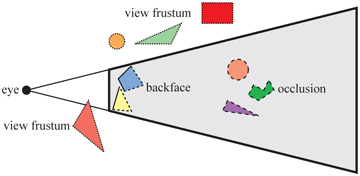
Figure 19.9. Different culling techniques. Culled geometry is dashed. (Illustration after Cohen-Or et al. [277].)
The actual culling can theoretically take place at any stage of the rendering pipeline, and for some occlusion culling algorithms, it can even be precomputed. For culling algorithms that are implemented on the GPU, we can sometimes only enable/disable, or set some parameters for, the culling function. The fastest triangle to render is the one never sent to the GPU. Next to that, the earlier in the pipeline culling can occur, the better. Culling is often achieved by using geometric calculations, but is in no way limited to these. For example, an algorithm may also use the contents of the frame buffer.
The ideal culling algorithm would send only the exact visible set (EVS) of primitives through the pipeline. In this book, the EVS is defined as all primitives that are partially or fully visible. One such data structure that allows for ideal culling is the aspect graph, from which the EVS can be extracted, given any point of view [532]. Creating such data structures is possible in theory, but not in practice, since worst-time complexity can be as bad as [277]. Instead, practical algorithms attempt to find a set, called the potentially visible set (PVS), that is a prediction of the EVS. If the PVS fully includes the EVS, so that only invisible geometry is discarded, the PVS is said to be conservative. A PVS may also be approximate, in which the EVS is not fully included. This type of PVS may therefore generate incorrect images. The goal is to make these errors as small as possible. Since a conservative PVS always generates correct images, it is often considered more useful. By overestimating or approximating the EVS, the idea is that the PVS can be computed much faster. The difficulty lies in how these estimations should be done to gain overall performance. For example, an algorithm may treat geometry at different granularities, i.e., triangles, whole objects, or groups of objects. When a PVS has been found, it is rendered using the z-buffer, which resolves the final per-pixel visibility.
Note that there are algorithms that reorder the triangles in a mesh in order to provide better occlusion culling, i.e., reduced overdraw, and improved vertex cache locality at the same time. While these are somewhat related to culling, we refer the interested reader to the references [256,659].
In Sections 19.3–19.8, we treat backface culling, view frustum culling, portal culling, detail culling, occlusion culling, and culling systems.
19.3 Backface Culling
Imagine that you are looking at an opaque sphere in a scene. Approximately half of the sphere will not be visible. The conclusion from this observation is that what is invisible need not be rendered since it does not contribute to the image. Therefore, the back side of the sphere need not be processed, and that is the idea behind backface culling. This type of culling can also be done for whole groups at a time, and so is called clustered backface culling.
All backfacing triangles that are part of a solid opaque object can be culled away from further processing, assuming the camera is outside of, and does not penetrate (i.e., near clip into), the object. A consistently oriented triangle (Section ) is backfacing if the projected triangle is known to be oriented in, say, a clockwise fashion in screen space. This test can be implemented by computing the signed area of the triangle in two-dimensional screen space. A negative signed area means that the triangle should be culled. This can be implemented immediately after the screen-mapping procedure has taken place.
Another way to determine whether a triangle is backfacing is to create a vector from an arbitrary point on the plane in which the triangle lies (one of the vertices is the simplest choice) to the viewer’s position. For orthographic projections, the vector to the eye position is replaced with the negative view direction, which is constant for the scene. Compute the dot product of this vector and the triangle’s normal. A negative dot product means that the angle between the two vectors is greater than radians, so the triangle is not facing the viewer. This test is equivalent to computing the signed If the sign is positive, the triangle is frontfacing. Note that the distance is obtained only if the normal is normalized, but this is unimportant here, as only the sign is of interest. Alternatively, after the projection matrix has been applied, form vertices in clip space and compute the determinant [1317]. If , the triangle can be culled. These culling techniques are illustrated in Figure 19.10.

Figure 19.10. Two different tests for determining whether a triangle is backfacing. The left figure shows how the test is done in screen space. The two triangles to the left are frontfacing, while the right triangle is backfacing and can be omitted from further processing. The right figure shows how the backface test is done in view space. Triangles A and B are frontfacing, while C is backfacing.
Blinn points out that these two tests are geometrically the same [165]. In theory, what differentiates these tests is the space where the tests are computed—nothing else. In practice, the screen-space test is often safer, because edge-on triangles that appear to face slightly backward in view space can become slightly forward in screen space. This happens because the view-space coordinates get rounded off to screen-space subpixel coordinates.
Using an API such as OpenGL or DirectX, backface culling is normally controlled with a few functions that either enable backface or frontface culling or disable all culling. Be aware that a mirroring transform (i.e., a negative scaling operation) turns backfacing triangles into frontfacing ones and vice versa [165] (Section ). Finally, it is possible to find out in the pixel shader whether a triangle is frontfacing. In OpenGL, this is done by testing gl_FrontFacing and in DirectX it is called SV_IsFrontFace. Prior to this addition the main way to display two-sided objects properly was to render them twice, first culling backfaces then culling frontfaces and reversing the normals.
A common misconception about standard backface culling is that it cuts the number of triangles rendered by about half. While backface culling will remove about half of the triangles in many objects, it will provide little gain for some types of models. For example, the walls, floor, and ceiling of interior scenes are usually facing the viewer, so there are relatively few backfaces of these types to cull in such scenes. Similarly, with terrain rendering often most of the triangles are visible, and only those on the back sides of hills or ravines benefit from this technique.
While backface culling is a simple technique for avoiding rasterizing individual triangles, it would be even faster if one could decide with a single test if a whole set of triangles could be culled.
Such techniques are called clustered backface culling algorithms, and some of these will be reviewed here. The basic concept that many such algorithms use is the normal cone [1630]. For some section of a surface, a truncated cone is created that contains all the normal directions and all the points. Note that two distances along the normal are needed to truncate the cone. See Figure 19.11 for an example.
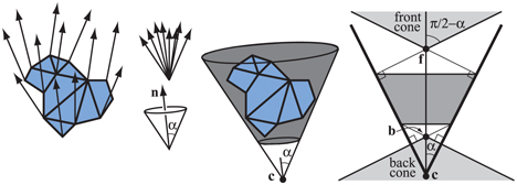
Figure 19.11. Left: a set of triangles and their normals. Middle left: the normals are collected (top), and a minimal cone (bottom), defined by one normal , and a half-angle, , is constructed. Middle right: the cone is anchored at a point , and truncated so that it also contains all points on the triangles. Right: a cross section of a truncated cone. The light gray region on the top is the frontfacing cone, and the light gray region at the bottom is the backfacing cone. The points and are respectively the apexes of the front- and backfacing cones.
As can be seen, a cone is defined by a normal, , and half-angle, , and an anchor point, , and some offset distances along the normal that truncates the cone. In the right part of Figure 19.11, a cross section of a normal cone is shown. Shirman and Abi-Ezzi [1630] prove that if the viewer is located in the frontfacing cone, then all faces in the cone are frontfacing, and similarly for the backfacing cone. Engel [433] uses a similar concept called the exclusion volume for GPU culling.
For static meshes, Haar and Aaltonen [625] suggest that a minimal cube is computed around n triangles, and each cube face is split into “pixels,” each encoding an n-bit mask that indicates whether the corresponding triangle is visible over that “pixel.” This is illustrated in Figure 19.12.
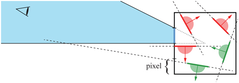
Figure 19.12. A set of five static triangles, viewed edge on, surrounded by a square in two dimensions. The square face to the left has been split into 4 “pixels,” and we focus on the one second from the top, whose frustum outside the box has been colored blue. The positive half-space formed by the triangle’s plane is indicated with a half-circle (red and green). All triangles that do not have any part of the blue frustum in its positive half-space are conservatively backfacing (marked red) from all points in the frustum. Green indicates those that are frontfacing
If the camera is outside the cube, one finds the corresponding frustum in which the camera is located and can immediately look up its bitmask and know which triangles are backfacing (conservatively). If the camera is inside the cube, all triangles are considered visible (unless one wants to perform further computations). Haar and Aaltonen use only one bitmask per cube face and encode triangles at a time. By counting the number of bits that are set in the bitmask, one can allocate memory for the non-culled triangles in an efficient manner. This work has been used in Assassin’s Creed Unity.
Next, we will use a non-truncated normal cone, in contrast to the one in Figure 19.11, and so it is defined by only a center point , normal , and an angle . To compute such a normal cone of a number of triangles, take all the normals of the triangle planes, put them in the same position, and compute a minimal circle on the unit sphere surface that includes all the normals [101]. As a first step, assume that from a point we want to backface-test all normals, sharing the same origin , in the cone. A normal cone is backfacing from if the following is true [1883,1884]:
(19.2)
However, this test only works if all the geometry is located at . Next, we assume that all geometry is inside a sphere with center point and radius r. The test then becomes
(19.3)
where . The geometry involved in deriving this test is shown in Figure 19.13. Quantized normals can be stored in bits, which may be sufficient for some applications.

Figure 19.13. This situation shows the limit when the normal cone, defined by , , and , is just about to become visible to from the most critical point inside the circle with radius r and center point . This happens when the angle between the vector from to a point on the circle such that the vector is tangent to the circle, and the side of the normal cone is radians. Note that the normal cone has been translated down from so its origin coincides with the sphere border.
To conclude this section, we note that backface culling for motion blurred triangles, where each vertex has a linear motion over a frame, is not as simple as one may think. A triangle with linearly moving vertices over time can be backfacing at the start of a frame, turn frontfacing, and then turn backfacing again, all within the same frame. Hence, incorrect results will be generated if a triangle is culled due to the motion blurred triangle being backfacing at the start and end of a frame. Munkberg and Akenine-Möller [1246] present a method where the vertices in the standard backface test are replaced with linearly moving triangles vertices. The test is rewritten in Bernstein form, and the convex property of Bézier curves is used as a conservative test. For depth of field, if the entire lens is in the negative half-space of the triangle (in other words, behind it), the triangle can be culled safely.
19.4 View Frustum Culling
As seen in Section 23.3, only primitives that are entirely or partially inside the view frustum need to be rendered. One way to speed up the rendering process is to compare the bounding volume of each object to the view frustum. If the BV is outside the frustum, then the geometry it encloses can be omitted from rendering. If instead the BV is inside or intersecting the frustum, then the contents of that BV may be visible and must be sent through the rendering pipeline. See Section for methods of testing for intersection between various bounding volumes and the view frustum.
By using a spatial data structure, this kind of culling can be applied hierarchically [272]. For a bounding volume hierarchy, a preorder traversal [292] from the root does the job. Each node with a bounding volume is tested against the frustum. If the BV of the node is outside the frustum, then that node is not processed further. The tree is pruned, since the BV’s contents and children are outside the view. If the BV is fully inside the frustum, its contents must all be inside the frustum. Traversal continues, but no further frustum testing is needed for the rest of such a subtree. If the BV intersects the frustum, then the traversal continues and its children are tested. When a leaf node is found to intersect, its contents (i.e., its geometry) is sent through the pipeline. The primitives of the leaf are not guaranteed to be inside the view frustum. An example of view frustum culling is shown in Figure 19.14.

Figure 19.14. A set of geometry and its bounding volumes (spheres) are shown on the left. This scene is rendered with view frustum culling from the point of the eye. The BVH is shown on the right. The BV of the root intersects the frustum, and the traversal continues with testing its children’s BVs. The BV of the left subtree intersects, and one of that subtree’s children intersects (and thus is rendered), and the BV of the other child is outside and therefore is not sent through the pipeline. The BV of the middle subtree of the root is entirely inside and is rendered immediately. The BV of the right subtree of the root is also fully inside, and the entire subtree can therefore be rendered without further tests.
It is also possible to use multiple BV tests for an object or cell. For example, if a sphere BV around a cell is found to overlap the frustum, it may be worthwhile to also perform the more accurate (though more expensive) OBB-versus-frustum test if this box is known to be much smaller than the sphere [1600].
A useful optimization for the “intersects frustum” case is to keep track of which frustum planes the BV is fully inside [148]. This information, usually stored as a bitmask, can then be passed with the intersector for testing children of this BV. This technique is sometimes called plane masking, as only those planes that intersected the BV need to be tested against the children. The root BV will initially be tested against all 6 frustum planes, but with successive tests the number of plane/BV tests done at each child will go down. Assarsson and Möller [83] note that temporal coherence can also be used. The frustum plane that rejects a BV could be stored with the BV and then be the first plane tested for rejection in the next frame. Wihlidal [1883,1884] notes that if view frustum culling is done on a per-object level on the CPU, then it suffices to perform view frustum culling against the left, right, bottom, and top planes when finer-grained culling is done on the GPU. Also, to improve performance, a construction called the apex point map can be used to provide tighter bounding volumes. This is described in more detail in Section 22.13.4. Sometimes fog is used in the distance to avoid the effect of objects suddenly disappearing at the far plane.
For large scenes or certain camera views, only a fraction of the scene might be visible, and it is only this fraction that needs to be sent through the rendering pipeline. In such cases a large gain in speed can be expected. View frustum culling techniques exploit the spatial coherence in a scene, since objects that are located near each other can be enclosed in a BV, and nearby BVs may be clustered hierarchically.
It should be noted that some game engines do not use hierarchical BVHs, but rather just a linear list of BVs, one for each object in the scene [283]. The main motivation is that it is simpler to implement algorithms using SIMD and multiple threads, so giving better performance. However, for some applications, such as CAD, most or all of the geometry is inside the frustum, in which case one should avoid using these types of algorithms. Hierarchical view frustum culling may still be applied, since if a node is inside the frustum, its geometry can immediately be drawn.
19.5 Portal Culling
For architectural models, there is a set of algorithms that goes under the name of portal culling. The first of these were introduced by Airey et al. [17,18]. Later, Teller and Séquin [1755,1756] and Teller and Hanrahan [1757] constructed more efficient and more complex algorithms for portal culling. The rationale for all portal-culling algorithms is that walls often act as large occluders in indoor scenes. Portal culling is thus a type of occlusion culling, discussed in the next section. This occlusion algorithm uses a view frustum culling mechanism through each portal (e.g., door or window). When traversing a portal, the frustum is diminished to fit closely around the portal. Therefore, this algorithm can be seen as an extension of view frustum culling as well. Portals that are outside the view frustum are discarded.
Portal-culling methods preprocess the scene in some way. The scene is divided into cells that usually correspond to rooms and hallways in a building. The doors and windows that connect adjacent rooms are called portals. Every object in a cell and the walls of the cell are stored in a data structure that is associated with the cell. We also store information on adjacent cells and the portals that connect them in an adjacency graph. Teller presents algorithms for computing this graph [1756]. While this technique worked back in 1992 when it was introduced, for modern complex scenes automating the process is extremely difficult. For that reason defining cells and creating the graph is currently done by hand.
Luebke and Georges [1090] use a simple method that requires just a small amount of preprocessing. The only information that is needed is the data structure associated with each cell, as described above. The key idea is that each portal defines the view into its room and beyond. Imagine that you are looking through a doorway to a room with three windows. The doorway defines a frustum, which you use to cull out the objects not visible in the room, and you render those that can be seen. You cannot see two of the windows through the doorway, so the cells visible through those windows can be ignored. The third window is visible but partially blocked by the doorframe. Only the contents in the cell visible through both the doorway and this window needs to be sent down the pipeline. The cell rendering process depends on tracking this visibility, in a recursive manner.

Figure 19.15. Portal culling: Cells are enumerated from A to H, and portals are openings that connect the cells. Only geometry seen through the portals is rendered. For example, the star in cell F is culled.
The portal culling algorithm is illustrated in Figure 19.15 with an example. The viewer or eye is located in cell E and therefore rendered together with its contents. The neighboring cells are C, D, and F. The original frustum cannot see the portal to cell D and is therefore omitted from further processing. Cell F is visible, and the view frustum is therefore diminished so that it goes through the portal that connects to F. The contents of F are then rendered with that diminished frustum. Then, the neighboring cells of F are examined—G is not visible from the diminished frustum and so is omitted, while H is visible. Again, the frustum is diminished with the portal of H, and thereafter the contents of H are rendered. H does not have any neighbors that have not been visited, so traversal ends there. Now, recursion falls back to the portal into cell C. The frustum is diminished to fit the portal of C, and then rendering of the objects in C follows, with frustum culling. No more portals are visible, so rendering is complete.
Each object may be tagged when it has been rendered, to avoid rendering objects more than once. For example, if there were two windows into a room, the contents of the room are culled against each frustum separately. Without tagging, an object visible through both windows would be rendered twice. This is both inefficient and can lead to rendering errors, such as when an object is transparent. To avoid having to clear this list of tags each frame, each object is tagged with the frame number when visited. Only objects that store the current frame number have already been visited.
An optimization that can well be worth implementing is to use the stencil buffer for more accurate culling. In practice, portals are overestimated with an AABB; the real portal will most likely be smaller. The stencil buffer can be used to mask away rendering outside that real portal. Similarly, a scissor rectangle around the portal can be set for the GPU to increase performance [13]. Using stencil and scissor functionality also obviates the need to perform tagging, as transparent objects may be rendered twice but will affect visible pixels in each portal only once.

Figure 19.16. Portal culling. The left image is an overhead view of the Brooks House. The right image is a view from the master bedroom. Cull boxes for portals are in white and for mirrors are in red. (Images courtesy of David Luebke and Chris Georges, UNC-Chapel Hill.)
See Figure 19.16 for another view of the use of portals. This form of portal culling can also be used to trim content for planar reflections (Section ). The left image shows a building viewed from the top; the white lines indicate the way in which the frustum is diminished with each portal. The red lines are created by reflecting the frustum at a mirror. The actual view is shown in the image on the right side, where the white rectangles are the portals and the mirror is red. Note that it is only the objects inside any of the frusta that are rendered. Other transformations can be used to create other effects, such as simple refractions.
19.6 Detail and Small Triangle Culling
Detail culling is a technique that sacrifices quality for speed. The rationale for detail culling is that small details in the scene contribute little or nothing to the rendered images when the viewer is in motion. When the viewer stops, detail culling is usually disabled. Consider an object with a bounding volume, and project this BV onto the projection plane. The area of the projection is then estimated in pixels, and if the number of pixels is below a user-defined threshold, the object is omitted from further processing. For this reason, detail culling is sometimes called screen-size culling. Detail culling can also be done hierarchically on a scene graph. These types of techniques are often used in game engines [283].
With one sample at the center of each pixel, small triangles are rather likely to fall between the samples. In addition, small triangles are rather inefficient to rasterize. Some graphics hardware actually cull triangles falling between samples, but when culling is done using code on the GPU (Section 19.8), it may be beneficial to add some code to cull small triangles. Wihlidal [1883,1884] presents a simple method, where the AABB of the triangle is first computed. The triangle can be culled in a shader if the following is true:
(19.4)
where min and max represent the two-dimensional AABB around the triangle. The function any returns true if any of the vector components are true. Recall also that pixel centers are located at , which means that Equation 19.4 is true if either the x- or y-coordinates, or both, round to the same coordinates. Some examples are shown in Figure 19.17.

Figure 19.17. Small triangle culling using any(round(min) == round(max)). Red triangles are culled, while green triangles need to be rendered. Left: the green triangle overlaps with a sample, so cannot be culled. The red triangles both round all AABB coordinates to the same pixel corners. Right: the red triangles can be culled because one of AABB coordinates is rounded to the same integer. The green triangle does not overlap any samples, but cannot be culled by this test.
19.7 Occlusion Culling
As we have seen, visibility may be solved via the z-buffer. Even though it solves visibility correctly, the z-buffer is relatively simple and brute-force, and so not always the most efficient solution. For example, imagine that the viewer is looking along a line where 10 spheres are placed. This is illustrated in Figure 19.18. An image rendered from this viewpoint will show but one sphere, even though all 10 spheres will be rasterized and compared to the z-buffer, and then potentially written to the color buffer and z-buffer. The middle part of Figure 19.18 shows the depth complexity for this scene from the given viewpoint. Depth complexity is the number of surfaces covered by a pixel. In the case of the 10 spheres, the depth complexity is 10 for the pixel in the middle as all 10 spheres are located there, assuming backface culling is on. If the scene is rendered back to front, the pixel in the middle will be pixel shaded 10 times, i.e., there are 9 unnecessary pixel shader executions. Even if the scene is rendered front to back, the triangles for all 10 spheres will still be rasterized, and depth will be computed and compared to the depth in the z-buffer, even though an image of a single sphere is generated. This uninteresting scene is not likely to be found in reality, but it describes (from the given viewpoint) a densely populated model. These sorts of configurations are found in real scenes such as those of a rain forest, an engine, a city, and the inside of a skyscraper. See Figure 19.19 for an example.
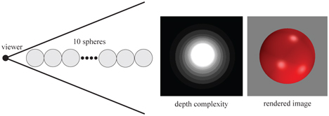
Figure 19.18. An illustration of how occlusion culling can be useful. Ten spheres are placed in a line, and the viewer is looking along this line (left) with perspective. The depth complexity image in the middle shows that some pixels are written to several times, even though the final image (on the right) only shows one sphere.

Figure 19.19. A Minecraft
Given the examples in the previous paragraph, it seems plausible that an algorithmic approach to avoid this kind of inefficiency may pay off in performance. Such approaches go under the name of occlusion culling algorithms, since they try to cull away objects that are occluded, that is, hidden by other objects in the scene. The optimal occlusion culling algorithm would select only the objects that are visible. In a sense, the z-buffer selects and renders only those objects that are visible, but not without having to send all objects inside the view frustum through most of the pipeline. The idea behind efficient occlusion culling algorithms is to perform some simple tests early on to cull sets of hidden objects. In a sense, backface culling is a simple form of occlusion culling. If we know in advance that an object is solid and is opaque, then the backfaces are occluded by the frontfaces and so do not need to be rendered.
There are two major forms of occlusion culling algorithms, namely point-based and cell-based. These are illustrated in Figure 19.20.

Figure 19.20. The left figure shows point-based visibility, while the right shows cell-based visibility, where the cell is a box. As can be seen, the circles are occluded to the left from the viewpoint. To the right, however, the circles are visible, since rays can be drawn from somewhere within the cell to the circles without intersecting any occluder.
Point-based visibility is just what is normally used in rendering, that is, what is seen from a single viewing location. Cell-based visibility, on the other hand, is done for a cell, which is a region of the space containing a set of viewing locations, normally a box or a sphere. An invisible object in cell-based visibility must be invisible from all points within the cell. The advantage of cell-based visibility is that once it is computed for a cell, it can usually be used for a few frames, as long as the viewer is inside the cell. However, it is usually more time consuming to compute than point-based visibility. Therefore, it is often done as a preprocessing step. Point-based and cell-based visibility are similar in nature to point and area light sources, where the light can be thought of as viewing the scene. For an object to be invisible, this is equivalent to it being in the umbra region, i.e., fully in shadow.
One can also categorize occlusion culling algorithms into those that operate in image space, object space, or ray space. Image-space algorithms do visibility testing in two dimensions after some projection, while object-space algorithms use the original three-dimensional objects. Ray-space methods [150,151,923] perform their tests in a dual space. Each point of interest, often two-dimensional, is converted to a ray in this dual space. For real-time graphics, of the three, image-space occlusion culling algorithms are the most widely used.

Figure 19.21. Pseudocode for a general occlusion culling algorithm. G contains all the objects in the scene, and is the occlusion representation. P is a set of potential occluders, that are merged into when it contains sufficiently many objects. (After Zhang [1965].)
Pseudocode for one type of occlusion culling algorithm is shown in Figure 19.21, where the function isOccluded, often called the visibility test, checks whether an object is occluded. G is the set of geometrical objects to be rendered, is the occlusion representation, and P is a set of potential occluders that can be merged with . Depending on the particular algorithm, represents some kind of occlusion information. is set to be empty at the beginning. After that, all objects (that pass the view frustum culling test) are processed.
Consider a particular object. First, we test whether the object is occluded with respect to the occlusion representation . If it is occluded, then it is not processed further, since we then know that it will not contribute to the image. If the object cannot be determined to be occluded, then that object has to be rendered, since it probably contributes to the image (at that point in the rendering). Then the object is added to P, and if the number of objects in P is large enough, then we can afford to merge the occluding power of these objects into . Each object in P can thus be used as an occluder.
Note that for most occlusion culling algorithms, the performance is dependent on the order in which objects are drawn. As an example, consider a car with a motor inside it. If the hood of the car is drawn first, then the motor will (probably) be culled away. On the other hand, if the motor is drawn first, then nothing will be culled. Sorting and rendering in rough front-to-back order can give a considerable performance gain. Also, it is worth noting that small objects potentially can be excellent occluders, since the distance to the occluder determines how much it can occlude. As an example, a matchbox can occlude the Golden Gate Bridge if the viewer is sufficiently close to the matchbox.
19.7.1. Occlusion Queries
GPUs support occlusion culling by using a special rendering mode. The user can query the GPU to find out whether a set of triangles is visible when compared to the current contents of the z-buffer. The triangles most often form the bounding volume (for example, a box or k-DOP) of a more complex object. If none of these triangles are visible, then the object can be culled. The GPU rasterizes the triangles of the query and compares their depths to the z-buffer, i.e., it operates in image space. A count of the number of pixels n in which these triangles are visible is generated, though no pixels nor any depths are actually modified. If n is zero, all triangles are occluded or clipped.
However, a count of zero is not quite enough to determine if a bounding volume is not visible. More precisely, no part of the camera frustum’s visible near plane should be inside the bounding volume. Assuming this condition is met, then the entire bounding volume is completely occluded, and the contained objects can safely be discarded. If , then a fraction of the pixels failed the test. If n is smaller than a threshold number of pixels, the object could be discarded as being unlikely to contribute much to the final image [1894]. In this way, speed can be traded for possible loss of quality. Another use is to let n help determine the LOD (Section 19.9) of an object. If n is small, then a smaller fraction of the object is (potentially) visible, and so a less-detailed LOD can be used.
When the bounding volume is found to be obscured, we gain performance by avoiding sending a potentially complex object through the rendering pipeline. However, if the test fails, we actually lose a bit of performance, as we spent additional time testing this bounding volume to no benefit.
There are variants of this test. For culling purposes, the exact number of visible fragments is not needed—it suffices with a boolean indicating whether at least one fragment passes the depth test. OpenGL 3.3 and DirectX 11 and later support this type of occlusion query, enumerated as ANY_SAMPLES_PASSED in OpenGL [1598]. These tests can be faster since they can terminate the query as soon as one fragment is visible. OpenGL 4.3 and later also allows a faster variant of this query, called ANY_SAMPLES_PASSED_CONSERVATIVE. The implementation may choose to provide a less-precise test as long as it is conservative and errs on the correct side. A hardware vendor could implement this by performing the depth test against only the coarse depth buffer (Section ) instead of the per-pixel depths, for example.
The latency of a query is often a relatively long time. Usually, hundreds or thousands of triangles can be rendered within this time—see Section for more about latency. Hence, this GPU-based occlusion culling method is worthwhile when the bounding boxes contain a large number of objects and a relatively large amount of occlusion is occurring. GPUs use an occlusion query model in which the CPU can send off any number of queries to the GPU, then it periodically checks to see if any results are available, that is, the query model is asynchronous. For its part, the GPU performs each query and puts the result in a queue. The queue check by the CPU is extremely fast, and the CPU can continue to send down queries or actual renderable objects without having to stall. Both DirectX and OpenGL support predicated/conditional occlusion queries, where both the query and an ID to the corresponding draw call are submitted at the same time. The corresponding draw call is automatically processed by the GPU only if it is indicated that the geometry of the occlusion query is visible. This makes the model substantially more useful.
In general, queries should be performed on objects most likely to be occluded. Kovalèík and Sochor [932] collect running statistics on queries over several frames for each object while the application is running. The number of frames in which an object was found to be hidden affects how often it is tested for occlusion in the future. That is, objects that are visible are likely to stay visible, and so can be tested less frequently. Hidden objects get tested every frame, if possible, since these objects are most likely to benefit from occlusion queries. Mattausch et al. [1136] present several optimizations for occlusion queries (OCs) without predicated/conditional rendering. They use batching of OCs, combining a few OCs into a single OC, use several bounding boxes instead of a single larger one, and use temporally jittered sampling for scheduling of previously visible objects.
The schemes discussed here give a flavor of the potential and problems with occlusion culling methods. When to use occlusion queries, or use most occlusion schemes in general, is not often clear. If everything is visible, an occlusion algorithm can only cost additional time, never save it. One challenge is rapidly determining that the algorithm is not helping, and so cutting back on its fruitless attempts to save time. Another problem is deciding what set of objects to use as occluders. The first objects that are inside the frustum must be visible, so spending queries on these is wasteful. Deciding in what order to render and when to test for occlusion is a struggle in implementing most occlusion-culling algorithms.
19.7.2. Hierarchical Z-Buffering
Hierarchical z-buffering (HZB) [591,593] has had significant influence on occlusion culling research. Though the original CPU-side form is rarely used, the algorithm is the basis for the GPU hardware method of z-culling (Section ) and for custom occlusion culling using software running on the GPU or on the CPU. We first describe the basic algorithm, followed by how the technique has been adopted in various rendering engines.
The algorithm maintains the scene model in an octree, and a frame’s z-buffer as an image pyramid, which we call a z-pyramid. The algorithm thus operates in image space. The octree enables hierarchical culling of occluded regions of the scene, and the z-pyramid enables hierarchical z-buffering of primitives. The z-pyramid is thus the occlusion representation of this algorithm. Examples of these data structures are shown in Figure 19.22.
The finest (highest-resolution) level of the z-pyramid is simply a standard z-buffer. At all other levels, each z-value is the farthest z in the corresponding window of the adjacent finer level. Therefore, each z-value represents the farthest z for a square region of the screen. Whenever a z-value is overwritten in the z-buffer, it is propagated through the coarser levels of the z-pyramid. This is done recursively until the top of the image pyramid is reached, where only one z-value remains. Pyramid formation is illustrated in Figure 19.23.

Figure 19.22. Example of occlusion culling with the HZB algorithm [591,593], showing a scene with high depth complexity (lower right) with the corresponding z-pyramid (on the left), and octree subdivision (upper right). By traversing the octree from front to back and culling occluded octree nodes as they are encountered, this algorithm visits only visible octree nodes and their children (the nodes portrayed at the upper right) and renders only the triangles in visible boxes. In this example, culling of occluded octree nodes reduces the depth complexity from 84 to 2.5. (Images courtesy of Ned Greene/Apple Computer.)

Figure 19.23. On the left, a piece of the z-buffer is shown. The numerical values are the actual z-values. This is downsampled to a region where each value is the farthest (largest) of the four regions on the left. Finally, the farthest value of the remaining four z-values is computed. These three maps compose an image pyramid that is called the hierarchical z-buffer.
Hierarchical culling of octree nodes is done as follows. Traverse the octree nodes in a rough front-to-back order. A bounding box of the octree is tested against the z-pyramid using an extended occlusion query (Section 19.7.1). We begin testing at the coarsest z-pyramid cell that encloses the box’s screen projection. The box’s nearest depth within the cell ( ) is then compared to the z-pyramid value, and if is farther, the box is known to be occluded. This testing continues recursively down the z-pyramid until the box is found to be occluded, or until the bottom level of the z-pyramid is reached, at which point the box is known to be visible. For visible octree boxes, testing continues recursively down in the octree, and finally potentially visible geometry is rendered into the hierarchical z-buffer. This is done so that subsequent tests can use the occluding power of previously rendered objects.
The full HZB algorithm is not used these days, but it has been simplified and adapted to work well with compute passes using custom culling on the GPU or using software rasterization on the CPU. In general, most occlusion culling algorithms based on HZB work like this:
- Generate a full hierarchical z-pyramid using some occluder representation.
- To test if an object is occluded, project its bounding volume to screen space and estimate the mip level in the z-pyramid.
- Test occlusion against the selected mip level. Optionally continue testing using a finer mip level if results are ambiguous.
Most implementations do not use an octree or any BVH, nor do they update the z-pyramid after an object has been rendered since this is considered too expensive to perform.
Step 1 can be done using the “best” occluders [1637], which could be selected as the closest set of n objects [625], using simplified artist-generated occluder primitives, or using statistics concerning the set of objects that were visible the previous frame. Alternatively, one may use the z-buffer from the previous frame [856], however this is not conservative in that objects may sometimes just pop up due to incorrect culling, especially under quick camera or object movement. Haar and Aaltonen [625] both render the best occluders and combine them with a reprojection of 1 / 16 low resolution of the previous frame’s depth. The z-pyramid is then constructed, as shown in Figure 19.23, using the GPU. Some use the HTILE of the AMD GCN architecture (Section ) to speed up z-pyramid generation [625].
In step 2, the bounding volume of an object is projected to screen space. Common choices for BVs are spheres, AABBs, and OBBs. The longest side, l (in pixels), of the projected BV is used to compute the mip level, , as [738,1637,1883,1884]
(19.5)
where n is the maximum number of mip levels in the z-pyramid. The operator is there to avoid getting negative mip levels, and the avoids accessing mip levels that do not exist. Equation 19.5 selects the lowest integer mip level such that the projected BV covers at most depth values. The reason for this choice is that it makes the cost predictable—at most four depth values need to be read and tested. Also, Hill and Collin [738] argue that this test can be seen as “probabilistic” in the sense that large objects are more likely to be visible than small ones, so there is no reason to read more depth values in those cases.
When reaching step 3, we know that the projected BV is bounded by a certain set of, at most, depth values at that mip level. For a given-sized BV, it may fall entirely inside one depth texel on the mip level. However, depending on how it falls on the grid, it may cover up to all four texels. The minimum depth of the BV is computed, either exactly or conservatively. With an AABB in view space, this depth is simply the minimum depth of the box, and for an OBB, one may project all vertices onto the view vector and select the smallest distance. For spheres, Shopf et al. [1637] compute the closest point on the sphere as , where is the sphere center in view space and r is the sphere radius. Note that if the camera is inside a BV, then the BV covers the entire screen and the object is then rendered. The minimum depth, , of the BV is compared to the (at most) depths in the hierarchical z-buffer, and if is always larger, then the BV is occluded. It is possible to stop testing here and just render the object if it was not detected as occluded.
One may also continue testing against the next deeper (higher-resolution) level in the pyramid. We can see if such testing is warranted by using another z-pyramid that stores the minimum depths. We test the maximum distance, , to the BV against the corresponding depths in this new buffer. If is smaller than all these depths, then the BV is definitely visible and can be rendered immediately. Otherwise, the and of the BV overlap the depth of the two hierarchical z-buffers, in which case Kaplanyan [856] suggests testing be continued on a higher-resolution mip level. Note that testing texels in the hierarchical z-buffer against a single depth is quite similar to percentage-closer filtering (Section ). In fact, the test can be done using bilinear filtering with percentage-closer filtering, and if the test returns a positive value, then at least one texel is visible.
Haar and Altonen [625] also present a two-pass method that always renders at least all visible objects. First, occlusion culling for all objects is done against the previous frame’s z-pyramid, and the “visible” objects are rendered. Alternatively, one can use the last frame’s visibility list to directly render the z-pyramid. While this is an approximation, all the objects that were rendered serve as an excellent guess for the “best” occluders for the current frame, especially in scenarios with high frame-to-frame coherency. The second pass takes the depth buffer of these rendered objects and creates a new z-pyramid. Then, the objects that were occlusion culled in the first pass are tested for occlusion, and rendered if not culled. This method generates a fully correct image even if the camera moves quickly or objects move rapidly over the screen. Kubisch and Tavenrath [944] use a similar method.
Doghramachi and Bucci [363] rasterize oriented bounding boxes of the occludees against the previous frame’s depth buffer, which has been downsampled and reprojected. They force the shader to use early-z (Section ), and for each box the visible fragments mark the object as visible in a buffer location, which is uniquely determined from the object ID [944]. This provides higher culling rates since oriented boxes are used and since per-pixel testing is done, instead of using a custom test against a mip level using Equation 19.5.
Collin [283] uses a float z-buffer (not hierarchical) and rasterizes artist-generated occluders with low complexity. This is done in software either using the CPU or using the SPUs (on PLAYSTATION 3) with highly optimized SIMD code. To perform occlusion testing, the screen-space AABB of an object is computed and its is compared against all relevant depths in the small z-buffer. Only objects that survive culling are sent to the GPU. This approach works but is not conservatively correct, since a lower resolution than the final framebuffer’s resolution is used. Wihlidal [1883] suggests that the low-resolution z-buffer also be used to load -values into the HiZ (Section ) of the GPU, e.g., priming the HTILE structure on AMD GCN. Alternatively, if HZB is used for compute-pass culling, then the software z-buffer can be used to generate the z-pyramid. In this way, the algorithms exploit all information generated in software.
Hasselgren et al. [683] present a different approach, where each tile has one bit per pixel and two -values [50], resulting in an overall cost of 3 bits per pixel. By using -values, it is possible to handle depth discontinuities better, since a background object can use one of the -values and a foreground object uses the other. This representation, called a masked hierarchical depth buffer (MHDB), is conservative and can also be used for -culling. Only coverage masks and a single maximum depth value are generated per tile during software triangle rasterization, which makes rasterization to the MHDB quick and efficient. During rasterization of triangles to the MDHB, occlusion testing of the triangles can be done to the MDHB as well, which optimizes the rasterizer. The MDHB is updated for each triangle, which is a strength that few of the other methods have. Two usage modes are evaluated. The first is to use special occlusion meshes and render these using the software rasterizer to the MDHB. After that, an AABB tree over the occludees is traversed and hierarchically tested against the MDHB. This can be highly effective, especially if there are many small objects in a scene. For the second approach, the entire scene is stored in an AABB tree and traversal of the scene is done in roughly front-to-back order using a heap. At each step, frustum culling and occlusion queries are done against the MDHB. The MDHB is also updated whenever an object is rendered. The scene in Figure 19.19 was rendered using this method. The open-source code is heavily optimized for AVX2 [683].
There are also middleware packages specifically for culling and for occlusion culling in particular. Umbra is one such framework, which has been integrated extensively with various game engines [13,1789].
19.8 Culling Systems
Culling systems have evolved considerably over the years, and continue to do so. In this section, we describe some overarching ideas and point to the literature for details. Some systems execute effectively all culling in the GPU’s compute shader, while others combine coarse culling on the CPU with a later finer culling on the GPU.
A typical culling system works on many granularities, as shown in Figure 19.24.

Figure 19.24. An example culling system that works on three different granularities. First, culling is done on a per-object level. Surviving objects are then culled on a per-cluster level. Finally, triangle culling is done, which is further described in Figure 19.25.
A cluster or chunk of an object is simply a subset of the triangles of the object. One may use triangle strips with 64 vertices [625], or groups of 256 triangles [1884], for example. At each step, a combination of culling techniques can be used. El Mansouri [415] uses small triangle culling, detail culling, view frustum culling, and occlusion culling on objects. Since a cluster is geometrically smaller than an object, it makes sense to use the same culling techniques even for clusters since they are more likely to be culled. One may use, for example, detail, frustum, clustered backface, and occlusion culling on clusters.
After culling has been done on a per-cluster level, one can perform an additional step where culling is done on a per-triangle level. To make this occur entirely on the GPU, the approach illustrated in Figure 19.25 can be used.

Figure 19.25. Triangle culling system, where a battery of culling algorithms first is applied to all individual triangles. To be able to use indirect drawing, i.e., without a GPU/CPU round trip, the surviving triangles are then compacted into a shorter list. This list is rendered by the GPU using indirect drawing.
Culling techniques for triangles include frustum culling after division by w, i.e., comparing the extents of the triangle against , backface testing, degenerate triangle culling, small triangle culling, and possibly occlusion culling as well. The triangles that remain after all the culling tests are then compacted into a minimal list, which is done in order to process only surviving triangles in the next step [1884]. The idea is to instruct the culling compute shader to send a draw command from the GPU to itself in this step. This is done using an indirect draw command. These calls are called “multi-draw indirect” in OpenGL and “execute indirect” in DirectX [433]. The number of triangles is written to a location in a GPU buffer, which together with the compacted list can be used by the GPU to render the list of triangles.
There are many ways to combine culling algorithms together with where they are executed, i.e., either on the CPU or on the GPU, and there are many flavors of each culling algorithm as well. The ultimate combination has yet to be found, but it is safe to say that the best approach depends on the target architecture and the content to be rendered. Next, we point to some important work in the field of CPU/GPU culling systems that has influenced the field substantially. Shopf et al. [1637] did all AI simulations for characters on the GPU, and as a consequence, the position of each character was only available in GPU memory. This led them to explore culling and LOD management using the compute shader, and most of the systems that followed have been heavily influenced by their work. Haar and Aaltonen [625] describe the system they developed for Assassin’s Creed Unity. Wihlidal [1883,1884] explains the culling system used in the Frostbite engine. Engel [433] presents a system for culling that helps improve a pipeline using a visibility buffer (Section ). Kubisch and Tavenrath [944] describe methods for rendering massive models with a large number of parts and optimize using different culling methods and API calls. One noteworthy method they use to occlusion-cull boxes is to create the visible sides of a bounding box using the geometry shader and then let early-z quickly cull occluded geometry.
19.9 Level of Detail
The basic idea of levels of detail (LODs) is to use simpler versions of an object as it makes less and less of a contribution to the rendered image. For example, consider a detailed car that may consist of a million triangles. This representation can be used when the viewer is close to the car. When the object is farther away, say covering only 200 pixels, we do not need all one million triangles. Instead, we can use a simplified model that has only, say, 1000 triangles. Due to the distance, the simplified version looks approximately the same as the more detailed version. See Figure 19.26. In this way, a significant performance increase can be expected. In order to reduce the total work involved in applying LOD techniques, they are best applied after culling techniques. For example, LOD selection is computed only for objects inside the view frustum.

Figure 19.26. Here, we show three different levels of detail for models of C4 explosives (top) and a Hunter (bottom). Elements are simplified or removed altogether at lower levels of detail. The small inset images show the simplified models at the relative sizes at which they might be used. (Top row of images courtesy of Crytek; bottom row courtesy of Valve Corp.)
LOD techniques can also be used in order to make an application work at the desired frame rates on a range of devices with different performance. On systems with lower speeds, less-detailed LODs can be used to increase performance. Note that while LOD techniques help first and foremost with a reduction in vertex processing, they also reduce pixel-shading costs. This occurs because the sum of all triangle edge lengths for a model will be lower, which means that quad overshading is reduced (Sections and ).
Fog and other participating media, described in Chapter 14, can be used together with LODs. This allows us to completely skip the rendering of an object as it enters fully opaque fog, for example. Also, the fogging mechanism can be used to implement time-critical rendering (Section 19.9.3). By moving the far plane closer to the viewer, more objects can be culled early on, increasing the frame rate. In addition, a lower LOD can often be used in the fog.
Some objects, such as spheres, Bézier surfaces, and subdivision surfaces, have levels of detail as part of their geometrical description. The underlying geometry is curved, and a separate LOD control determines how it is tessellated into displayable triangles. See Section for algorithms that adapt the quality of tessellations for parametric surfaces and subdivision surfaces.
In general, LOD algorithms consist of three major parts, namely, generation, selection, and switching. LOD generation is the part where different representations of a model are generated with varying amounts of detail. The simplification methods discussed in Section can be used to generate the desired number of LODs. Another approach is to make models with different numbers of triangles by hand. The selection mechanism chooses a level of detail model based on some criteria, such as estimated area on the screen. Finally, we need to change from one level of detail to another, and this process is termed LOD switching. Different LOD switching and selection mechanisms are presented in this section.
While the focus in this section is on choosing among different geometric representations, the ideas behind LODs can also be applied to other aspects of the model, or even to the rendering method used. Lower level of detail models can also use lower-resolution textures, thereby further saving memory as well as possibly improving cache access [240]. Shaders themselves can be simplified depending on distance, importance, or other factors [688,1318,1365,1842]. Kajiya [845] presents a hierarchy of scale showing how surface lighting models overlap texture mapping methods, which in turn overlap geometric details. Another technique is that fewer bones can be used for skinning operations for distant objects.
When static objects are relatively far away, billboards and impostors (Section ) are a natural way to represent them at little cost [1097]. Other surface rendering methods, such as bump or relief mapping, can be used to simplify the representation of a model. Figure 19.27 gives an example. Teixeira [1754] discusses how to bake normal maps onto surfaces using the GPU. The most noticeable flaw with this simplification technique is that the silhouettes lose their curvature. Loviscach [1085] presents a method of extruding fins along silhouette edges to create curved silhouettes.

Figure 19.27. On the left, the original model consists of 1.5 million triangles. On the right, the model has 1100 triangles, with surface details stored as heightfield textures and rendered using relief mapping. (Image courtesy of Natalya Tatarchuk, ATI Research, Inc.)
An example of the range of techniques that can be used to represent an object comes from Lengyel et al. [1030,1031]. In this research, fur is represented by geometry when extremely close up, by alpha-blended polylines when farther away, then by a blend with volume texture “shells,” and finally by a texture map when far away. See Figure 19.28. Knowing when and how best to switch from one set of modeling and rendering techniques to another and so maximize frame rate and quality is still an art and an open area for exploration.

Figure 19.28. From a distance, the bunny’s fur is rendered with volumetric textures. When the bunny comes closer, the hair is rendered with alpha-blended polylines. When close up, the fur along the silhouette is rendered with graftal fins. (Image courtesy of Jed Lengyel and Michael Cohen, Microsoft Research.)
19.9.1. LOD Switching
When switching from one LOD to another, an abrupt model substitution is often noticeable and distracting. This difference is called popping. Several different ways to perform this switching will be described here, and they each have different popping traits.
Discrete Geometry LODs
In the simplest type of LOD algorithm, the various representations are models of the same object containing different numbers of primitives. This algorithm is well suited for modern graphics hardware [1092], because these separate static meshes can be stored in GPU memory and reused (Section ). A more detailed LOD has a higher number of primitives. Three LODs of objects are shown in Figures 19.26 and 19.29. The first figure also shows the LODs at different distances from the viewer.

Figure 19.29. A part of a cliff at three different levels of detail, with 72,200, 13,719, and 7,713 triangles from left to right. (Images courtesy of Quixel Megascans.)
The switching from one LOD to another is sudden. That is, on the current frame a certain LOD is used, then on the next frame, the selection mechanism selects another LOD and immediately uses that for rendering. Popping is typically the worst for this type of LOD method, but it can work well if switching occurs at distances when the difference in the rendered LODs is barely visible. Better alternatives are described next.
Blend LODs
Conceptually, a simple way to switch is to do a linear blend between the two LODs over a short period of time. Doing so will certainly make for a smoother switch. Rendering two LODs for one object is naturally more expensive than just rendering one LOD, so this somewhat defeats the purpose of LODs. However, LOD switching usually takes place during only a short amount of time, and often not for all objects in a scene at the same time, so the quality improvement may well be worth the cost.
Assume a transition between two LODs—say LOD1 and LOD2—is desired, and that LOD1 is the current LOD being rendered. The problem is in how to render and blend both LODs in a reasonable fashion. Making both LODs semitransparent will result in a semitransparent (though somewhat more opaque) object being rendered to the screen, which looks strange.
Giegl and Wimmer [528] propose a blending method that works well in practice and is simple to implement. First draw LOD1 opaquely to the framebuffer (both color and z). Then fade in LOD2 by increasing its alpha value from 0 to 1 and using the “over” blend mode. When LOD2 has faded in so it is completely opaque, it is turned into the current LOD, and LOD1 is then faded out. The LOD that is being faded (in or out) should be rendered with the z-test enabled and z-writes disabled. To avoid distant objects that are drawn later drawing over the results of rendering the faded LOD, simply draw all faded LODs in sorted order after all opaque content, as is normally done for transparent objects. Note that in the middle of the transition, both LODs are rendered opaquely, one on top of the other. This technique works best if the transition intervals are kept short, which also helps keep the rendering overhead small. Mittring [1227] discusses a similar method, except that screen-door transparency (potentially at the subpixel level) is used to dissolve between versions.
Scherzer and Wimmer [1557] avoid rendering both LODs by only updating one of the LODs on each frame and reuse the other LOD from the previous frame. Backprojection of the previous frame is performed together with a combination pass using visibility textures. Faster rendering and better-behaved transitions are the main results.
Some objects lend themselves to other switching techniques. For example, the SpeedTree package [887] smoothly shifts or scales parts of their tree LOD models to avoid pops. See Figure 19.30 for one example. A set of LODs are shown in Figure 19.31, along with a billboard LOD technique used for distant trees.

Figure 19.30. Tree branches (and their leaves, not shown) are shrunk and then removed as the viewer moves away from the tree model. (Images courtesy of SpeedTree.)

Figure 19.31. Tree LOD models, near to far. When the tree is in the distance, it is represented by one of a set of billboards, shown on the right. Each billboard is a rendering of the tree from a different view, and consists of a color and normal map. The billboard most facing the viewer is selected. In practice 8 to 12 billboards are formed (6 are shown here), and the transparent sections are trimmed away to avoid spending time discarding fully transparent pixels (Section ). (Images courtesy of SpeedTree.)
Alpha LODs
A simple method that avoids popping altogether is to use what we call alpha LODs. This technique can be used by itself or combined with other LOD switching techniques. It is used on the simplest visible LOD, which can be the original model if only one LOD is available. As the metric used for LOD selection (e.g., distance to this object) increases, the overall transparency of the object is increased ( is decreased), and the object finally disappears when it reaches full transparency ( ). This happens when the metric value is larger than a user-defined invisibility threshold. When the invisibility threshold has been reached, the object need not be sent through the rendering pipeline at all as long as the metric value remains above the threshold. When an object has been invisible and its metric falls below the invisibility threshold, then it decreases its transparency and starts to be visible again. An alternative is to use the hysteresis method described in Section 19.9.2.
The advantage of using this technique standalone is that it is experienced as much more continuous than the discrete geometry LOD method, and so avoids popping. Also, since the object finally disappears altogether and need not be rendered, a significant speedup can be expected. The disadvantage is that the object entirely disappears, and it is only at this point that a performance increase is obtained. Figure 19.32 shows an example of alpha LODs.

Figure 19.32. The cone in the middle is rendered using an alpha LOD. The transparency of the cone is increased when the distance to it increases, and it finally disappears. The images on the left are shown from the same distance for viewing purposes, while the images to the right of the line are shown at different sizes.
One problem with using alpha transparency is that sorting by depth needs to be done to ensure transparent objects blend correctly. To fade out distant vegetation, Whatley [1876] discusses how a noise texture can be used for screen-door transparency. This has the effect of a dissolve, with more texels on the object disappearing as the distance increases. While the quality is not as good as a true alpha fade, screen-door transparency means that no sorting or blending is necessary.
CLODs and Geomorph LODs
The process of mesh simplification can be used to create various LOD models from a single complex object. Algorithms for performing this simplification are discussed in Section 16.5.1. One approach is to create a set of discrete LODs and use these as discussed previously. However, edge collapse methods have a property that allows other ways of making a transition between LODs. Here, we present two methods that exploit such information. These are useful as background, but are currently rarely used in practice.
A model has two fewer triangles after each edge collapse operation is performed. What happens in an edge collapse is that an edge is shrunk until its two endpoints meet and it disappears. If this process is animated, a smooth transition occurs between the original model and its slightly simplified version. For each edge collapse, a single vertex is joined with another. Over a series of edge collapses, a set of vertices move to join other vertices. By storing the series of edge collapses, this process can be reversed, so that a simplified model can be made more complex over time. The reversal of an edge collapse is called a vertex split. So, one way to change the level of detail of an object is to precisely base the number of triangles visible on the LOD selection value. At 100 meters away, the model might consist of 1000 triangles, and moving to 101 meters, it might drop to 998 triangles. Such a scheme is called a continuous level of detail (CLOD) technique. There is not, then, a discrete set of models, but rather a huge set of models available for display, each one with two less triangles than its more complex neighbor.
While appealing, using such a scheme in practice has some drawbacks. Not all models in the CLOD stream look good. Triangle meshes, which can be rendered much more rapidly than single triangles, are more difficult to use with CLOD techniques than with static models. If there are several instances of the same object in the scene, then each CLOD object needs to specify its own specific set of triangles, since it does not match any others. Forsyth [481] discuss solutions to these and other problems. While most CLOD techniques are rather serial in nature, they are not automatically a good fit for implementation on GPUs. Therefore, Hu et al. [780] present a modification of CLOD that better fits the parallel nature of the GPU. Their technique is also view-dependent in that if an object intersects, say, the left side of the view frustum, fewer triangles can be used outside the frustum, connecting to a higher-density mesh inside.
In a vertex split, one vertex becomes two. What this means is that every vertex on a complex model comes from some vertex on a simpler version. Geomorph LODs [768] are a set of discrete models created by simplification, with the connectivity between vertices maintained. When switching from a complex model to a simple one, the complex model’s vertices are interpolated between their original positions and those of the simpler version. When the transition is complete, the simpler level of detail model is used to represent the object. See Figure 19.33 for an example of a transition.

Figure 19.33. The left and right images show a low-detail model and a higher-detail model. The image in the middle shows a geomorph model interpolated approximately halfway between the left and right models. Note that the cow in the middle has equally many vertices and triangles as the model to the right. (Images generated using Melax’s “Polychop” simplification demo [1196].)
There are several advantages to geomorphs. The individual static models can be selected in advance to be of high quality, and easily can be turned into triangle meshes. Like CLOD, popping is also avoided by smooth transitions. The main drawback is that each vertex needs to be interpolated; CLOD techniques usually do not use interpolation, so the set of vertex positions themselves never changes. Another drawback is that the objects always appear to be changing, which may be distracting. This is especially true for textured objects. Sander and Mitchell [1543] describe a system in which geomorphing is used in conjunction with static, GPU-resident vertex and index buffers. It is also possible to combine the screen-door transparency of Mittring [1227] (described above) with geomorphs for an even smoother transition.
A related idea called fractional tessellation is supported by GPUs. In such schemes, the tessellation factor for a curved surface can be set to any floating point number, and so popping can be avoided. Fractional tessellation can be used for Bézier patches and displacement mapping primitives, for example. See Section for more on these techniques.
19.9.2. LOD Selection
Given that different levels of detail of an object exist, a choice must be made for which one of them to render, or which ones to blend. This is the task of LOD selection, and a few different techniques for this will be presented here. These techniques can also be used to select good occluders for occlusion culling algorithms.
In general, a metric, also called the benefit function, is evaluated for the current viewpoint and the location of the object, and the value of this metric picks an appropriate LOD. This metric may be based on, for example, the projected area of the bounding volume of the object or the distance from the viewpoint to the object. The value of the benefit function is denoted r here. See also Section on how to rapidly estimate the projection of a line onto the screen.
Range-Based
A common way of selecting a LOD is to associate the different LODs of an object with different distance ranges. The most detailed LOD has a range from zero to some user-defined value , which means that this LOD is visible when the distance to the object is less than . The next LOD has a range from to where . If the distance to the object is greater than or equal to and less than , then this LOD is used, and so on. Examples of four different LODs with their ranges, and their corresponding LOD node used in a scene graph, are illustrated in Figure 19.34.

Figure 19.34. The left part of this illustration shows how range-based LODs work. Note that the fourth LOD is an empty object, so when the object is farther away than , nothing is drawn, because the object is not contributing enough to the image to be worth the effort. The right part shows a LOD node in a scene graph. Only one of the children of a LOD node is descended based on r.

Figure 19.35. The colored areas illustrate the hysteresis regions for the LOD technique.
Unnecessary popping can occur if the metric used to determine which LOD to use varies from frame to frame around some value, . A rapid cycling back and forth between levels can occur. This can be solved by introducing some hysteresis around the value [898,1508]. This is illustrated in Figure 19.35 for a range-based LOD, but applies to any type. Here, the upper row of LOD ranges are used only when r is increasing. When r is decreasing, the bottom row of ranges is used.
Blending two LODs in the transition ranges is illustrated in Figure 19.36. However, this is not ideal, since the distance to an object may reside in the transition range for a long time, which increases the rendering burden due to blending two LODs. Instead, Mittring [1227] performs LOD switching during a finite amount of time, when the object reaches a certain transition range. For best results, this should be combined with the hysteresis approach above.

Figure 19.36. The colored areas illustrate ranges where blending is done between the two closest LODs, where b01 means blend between LOD0 and LOD1, for example, and LODk means that only LODk is rendered in the corresponding range.
Projected Area-Based
Another common metric for LOD selection is the projected area of the bounding volume, or an estimation of it. Here, we will show how the number of pixels of that area, called the screen-space coverage, can be estimated for spheres and boxes with perspective viewing.
Starting with spheres, the estimation is based on the fact that the size of the projection of an object diminishes with the distance from the viewer along the view direction. This is shown in Figure 19.37, which illustrates how the size of the projection is halved if the distance from the viewer is doubled, which holds for planar objects facing the viewer.

Figure 19.37. This illustration shows how the size of the projection of objects, without any thickness, is halved when the distance is doubled.
We define a sphere by its center point and a radius r. The viewer is located at looking along the normalized direction vector . The distance from to along the view direction is simply the projection of the sphere’s center onto the view vector: . We also assume that the distance from the viewer to the near plane of the view frustum is n. The near plane is used in the estimation so that an object that is located on the near plane returns its original size. The estimation of the radius of the projected sphere is then
(19.6)
The area of the projection in pixels is thus , where is the screen resolution. A higher value selects a more detailed LOD. This is an approximation. In fact, the projection of a three-dimensional sphere is an ellipse, as shown by Mara and McGuire [1122]. They also derive a method for computing conservative bounding polygons even in the case when the sphere intersects the near plane.
It is common practice to simply use a bounding sphere around an object’s bounding box. Another estimate is to use the screen bounds of the bounding box. However, thin or flat objects can vary considerably in the amount of projected area actually covered. For example, imagine a strand of spaghetti that has one end at the upper left corner of the screen, the other at the lower right. Its bounding sphere will cover the screen, as do the minimum and maximum two-dimensional screen bounds of its bounding box.
Schmalstieg and Tobler [1569] present a rapid routine for calculating the projected area of a box. The idea is to classify the viewpoint of the camera with respect to the box, and to use this classification to determine which projected vertices are included in the silhouette of the projected box. This process is done via a lookup table. Using these vertices, the area in view can be computed. The classification is categorized into three major cases, shown in Figure 19.38.

Figure 19.38. Three cases of projection of a cube, showing (from left to right) one, two, and three frontfaces. The outlines consist of four, six, and six vertices, respectively, and the area of each outline is computed for each polygon formed. (Illustration after Schmalstieg and Tobler [1569].)
Practically, this classification is done by determining on which side of the planes of the bounding box the viewpoint is located. For efficiency, the viewpoint is transformed into the coordinate system of the box, so that only comparisons are needed for classification. The result of the comparisons are put into a bitmask, which is used as an index into the LUT. This LUT determines how many vertices there are in the silhouette as seen from the viewpoint. Then, another lookup is used to actually find the silhouette vertices. After they have been projected to the screen, the area of the outline is computed. To avoid (sometimes drastic) estimation errors, it is worthwhile to clip the polygon formed to the view frustum’s sides. Source code is available on the web. Lengyel [1026] presents an optimization to this scheme, where a more compact LUT can be used.
It is not always a good idea to base the LOD selection on range or projection alone. For example, if an object has a certain AABB with some large and some small triangles in it, then the small triangles may alias badly and decrease performance due to quad overshading. If another object has the exact same AABB but with medium and large triangles in it, then both range-based and projection-based selection methods will select the same LOD. To avoid this, Schulz and Mader [1590] use the geometric mean, g, to help select the LOD:
(19.7)
where are the sizes of the triangles of the object. The reason to use a geometric mean instead of an arithmetic mean (average) is that many small triangles will make g smaller even if there are a few large triangles. This value is computed offline for the highest-resolution model, and is used to precompute a distance where the first switch should occur. The subsequent switch distances are simple functions of the first distance. This allows their system to use lower LODs more often, which increases performance.
Another approach is to compute the geometric error of each discrete LOD, i.e., an estimation of how many meters that simplified model deviates at most from the original model. This distance can then be projected to determine what the effect is in screen space to use that LOD. The lowest LOD, that also meets a user-defined screen-space error, is then selected.
Other Selection Methods
Range-based and projected area-based LOD selection are typically the most common metrics used. However, many others are possible, and we will mention a few here. Besides projected area, Funkhouser and Séquin [508] also suggest using the importance of an object (e.g., walls are more important than a clock on the wall), motion, hysteresis (when switching LODs, the benefit is lowered), and focus. This last, the viewer’s focus of attention, can be an important factor. For example, in a sports game, the figure controlling the ball is where the user will be paying the most attention, so the other characters can have relatively lower levels of detail [898]. Similarly, when eye tracking is used in a virtual reality application, higher LODs should be used where the viewer looks.
Depending on the application, other strategies may be fruitful. Overall visibility can be used, e.g., a nearby object seen through dense foliage can be rendered with a lower LOD. More global metrics are possible, such as limiting the overall number of highly detailed LODs used in order to stay within a given triangle budget [898]. See the next section for more on this topic. Other factors are visibility, colors, and textures. Perceptual metrics can also be used to choose a LOD [1468].
McAuley [1154] presents a vegetation system, where trunk and leaf clusters have three LODs before they become impostors. He preprocesses visibility, from different viewpoints and from different distances, between clusters for each object. Since a cluster in the back of the tree may be quite hidden by closer clusters, it is possible to select lower LODs for such clusters even if the tree is up close. For grass rendering, it is common to use geometry close to the viewer, billboards a bit farther away, and a simple ground texture at significant distances [1352].
19.9.3. Time-Critical LOD Rendering
It is often a desirable feature of a rendering system to have a constant frame rate. In fact, this is what often is referred to as “hard real-time” or time-critical rendering.. Such a system is given a specific amount of time, say 16 ms, and must complete its task (e.g., render the image) within that time. When time is up, the system has to stop processing. A hard real-time rendering system will be able to show the user more or all of the scene each frame if the objects in a scene are represented by LODs, versus drawing only a few highly detailed models in the time allotted.
Funkhouser and Séquin [508] have presented a heuristic algorithm that adapts the selection of the level of detail for all visible objects in a scene to meet the requirement of constant frame rate. This algorithm is predictive in the sense that it selects the LOD of the visible objects based on desired frame rate and on which objects are visible. Such an algorithm contrasts with a reactive algorithm, which bases its selection on the time it took to render the previous frame.
An object is called O and is rendered at a level of detail called L, which gives (O, L) for each LOD of an object. Two heuristics are then defined. One heuristic estimates the cost of rendering an object at a certain level of detail: . Another estimates the benefit of an object rendered at a certain level of detail: . The benefit function estimates the contribution to the image of an object at a certain LOD.
Assume the objects inside or intersecting the view frustum are called S. The main idea behind the algorithm is then to optimize the selection of the LODs for the objects S using the heuristically chosen functions. Specifically, we want to maximize
(19.8)
under the constraint
(19.9)
where T is the target frame time. In other words, we want to select the level of detail for the objects that gives us “the best image” within the desired frame rate. Next we describe how the cost and benefit functions can be estimated, and then we present an optimization algorithm for the above equations.
Both the cost function and the benefit function are hard to define so that they work under all circumstances. The cost function can be estimated by timing the rendering of a LOD several times with different viewing parameters. See Section for different benefit functions. In practice, the projected area of the BV of the object may suffice as a benefit function.
Finally, we will discuss how to choose the level of detail for the objects in a scene. First, we note the following: For some viewpoints, a scene may be too complex to be able to keep up with the desired frame rate. To solve this, we can define a LOD for each object at its lowest detail level, which is simply an object with no primitives—i.e., we avoid rendering the object [508]. Using this trick, we render only the most important objects and skip the unimportant ones.
To select the “best” LODs for a scene, Equation 19.8 has to be optimized under the constraint shown in Equation 19.9. This is an NP-complete problem, which means that to solve it correctly, the only thing to do is to test all different combinations and select the best. This is clearly infeasible for any kind of algorithm. A simpler, more feasible approach is to use a greedy algorithm that tries to maximize the for each object. This algorithm treats all the objects inside the view frustum and chooses to render the objects in descending order, i.e., the one with the highest value first. If an object has the same value for more than one LOD, then the LOD with the highest benefit is selected and rendered. This approach gives the most “bang for the buck.” For n objects inside the view frustum, the algorithm runs in time, and it produces a solution that is at least half as good as the best [507,508]. It is also possible to exploit frame-to-frame coherence to speed up the sorting of the values.
More information about LOD management and the combination of LOD management and portal culling can be found in Funkhouser’s PhD thesis [507]. Maciel and Shirley [1097] combine LODs with impostors and present an approximately constant-time algorithm for rendering outdoor scenes. The general idea is that a hierarchy of different representations (e.g., a set of LODs and hierarchical impostors) of an object is used. Then the tree is traversed in some fashion to give the best image given a certain amount of time. Mason and Blake [1134] present an incremental hierarchical LOD selection algorithm. Again, the different representations of an object can be arbitrary. Eriksson et al. [441] present hierarchical levels of detail (HLODs). Using these, a scene can be rendered with constant frame rate as well, or rendered such that the rendering error is bounded. Related to this is rendering on a power budget. Wang et al. [1843] present an optimization framework that selects good parameters for reducing power usage, which is important for mobile phones and tablets.
Related to time-critical rendering is another set of techniques that apply to static models. When the camera is not moving, the full model is rendered and accumulation buffering can be used for antialiasing, depth of field, and soft shadows, with a progressive update. However, when the camera moves, the levels of detail of all objects can be lowered and detail culling can be used to completely cull small objects in order to meet a certain frame rate.
19.10 Rendering Large Scenes
So far it has been implied that the scene to be rendered fits into the main memory of the computer. This may not always be the case. Some consoles only have 8 GB of internal memory, for example, while some game worlds can consist of hundreds of gigabytes of data. Therefore, we present methods for streaming and transcoding of textures, some general streaming techniques, and finally terrain rendering algorithms. Note that these methods are almost always combined with culling techniques and level of detail methods, described earlier in this chapter.
19.10.1. Virtual Texturing and Streaming
Imagine that you want to use a texture with an incredibly large resolution in order to be able to render a huge terrain data set, and that this texture is so large that it does not fit into GPU memory. As an example, some virtual textures in the game RAGE have a resolution of , which would consume 64 GB of GPU memory [1309]. When memory is limited on the CPU, operating systems use virtual memory for memory management, swapping in data from the drive to CPU memory as needed [715]. This functionality is what sparse textures [109,248] provide, making it possible to allocate a huge virtual texture, also known as a megatexture. These sets of techniques are sometimes called virtual texturing or partially resident texturing. The application determines which regions (tiles) of each mipmap level should be resident in GPU memory. A tile is typically 64 kB and its texture resolution depends on the texture format. Here, we present virtual texturing and streaming techniques.
The key observation about an efficient texturing system using mipmapping is that the number of texels needed should ideally be proportional to the resolution of the final image being rendered, independent of the resolutions of the textures themselves. As a consequence, we only require the texels that are visible to be located in physical GPU memory, which is a rather limited set compared to all texels in an entire game world. The main concept is illustrated in Figure 19.39, where the entire mipmap chain is divided into tiles in both virtual and physical memory. These structures are sometimes called virtual mipmaps or clipmaps [1739], where the latter term refers to a smaller part of the larger mipmap being clipped out for use.

Figure 19.39. In virtual texturing, a large virtual texture with its mipmap hierarchy is divided into tiles (left) of, say, pixels each. Only a small set ( tiles in this case) can fit into physical memory (right). To find the location of a virtual texture tile, a translation from a virtual address to physical address is required, which here is done via a page table. Note that, in order to reduce clutter, not all tiles in physical memory have arrows from the virtual texture. (Image texture of the Bazman volcano, Iran. From NASA’s “Visible Earth” project.)
Since the size of physical memory is much smaller than virtual memory, only a small set of the virtual texture tiles can fit into the physical memory. The geometry uses a global uv-parameterization into the virtual texture, and before such uv-coordinates are used in a pixel shader, they need to be translated into texture coordinates that point into physical texture memory. This is done using either a GPU-supported page table (shown in Figure 19.39) or an indirection texture, if done in software on the GPU. The GPU in the Nintendo GameCube has virtual texture support. More recently, the PLAYSTATION 4, Xbox One, and many other GPUs have support for hardware virtual texturing. The indirection texture needs to be updated with correct offsets as tiles are mapped and unmapped to physical memory. Using a huge virtual texture and a small physical texture works well because distant geometry only needs to load a few higher-level mipmap tiles into physical memory, while geometry close to the camera can load a few lower-level mipmap tiles. Note that virtual texturing can be used for streaming huge textures from disk but also for sparse shadow mapping [241], for example.
Since physical memory is limited, all engines using virtual texturing need a way to determine which tiles should be resident, i.e., located in physical memory, and which should not. There are several such methods. Sugden and Iwanicki [1721] use a feedback rendering approach, where a first render pass writes out all the information required to know which texture tile a fragment will access. When that pass is done, the texture is read back to the CPU and analyzed to find which tiles are needed. The tiles that are not resident are read and mapped to physical memory, and tiles in physical memory that are not needed are unmapped. Their approach does not work for shadows, reflections, and transparency. However, screen-door techniques (Section ) can be used for transparent effects, which work reasonably well. Feedback rendering is also used by van Waveren and Hart [1855]. Note that such a pass could either be a separate rendering pass or be combined with a z-prepass. When a separate pass is used, a resolution of only pixels can be used, as an approximation, to reduce processing time. Hollemeersch et al. [761] use a compute pass instead of reading back the feedback buffer to the CPU. The result is a compact list of tile identifiers created on the GPU, and sent back to the CPU for mapping.
With GPU-supported virtual texturing, it is the responsibility of the driver to create and destroy resources, to map and unmap tiles, and to make sure that physical allocations are backed by virtual allocations [1605]. With GPU-hardware virtual texturing, a sparseTexture lookup returns a code indicating whether the corresponding tile is resident, in addition to the filtered value (for resident tiles) [1605]. With software-supported virtual texturing, all these tasks fall back on the developer. We refer to van Waveren’s report for more information on this topic [1856].
To make sure everything fits into physical memory, van Waveren adjusts a global texture LOD bias until the working set fits [1854]. In addition, when only a higher-level mipmap tile is available than what is desired, that higher-level mipmap tile needs to be used until the lower-level mipmap tile becomes available. In such cases, the higher-level mipmap tile can be upscaled immediately and used, and then the new tile can be blended in over time to make for a smooth transition when it becomes available.
Barb [99] instead always loads all textures that are smaller than or equal to 64 kB, and hence, some texturing can always be done, albeit at lower quality if the higher-resolution mipmap levels have not yet been loaded. He uses offline feedback rendering to precompute, for various locations, how much solid angle around the player each mipmap level covers for each material at a nominal texture and screen resolution. At runtime this information is streamed in and adjusted for both the resolution of each texture with that material and the final screen resolution. This yields an importance value per texture, per mipmap. Each importance value is then divided by the number of texels in the corresponding mipmap level, which generates a reasonable final metric since it is invariant even if a texture is subdivided into smaller, identically mapped textures. See Barb’s presentation for more information [99]. An example rendering is shown in Figure 19.40.

Figure 19.40. High-resolution texture mapping accessing a huge image database using texture streaming in DOOM (2016). (Image from the game “DOOM,” courtesy of id Software.)
Widmark [1881] describes how streaming can be combined with procedural texture generation for a more varied and detailed texture. Chen extends Widmark’s scheme to handle textures an order of magnitude larger [259].
19.10.2. Texture Transcoding
To make a virtual texturing system work even better, it can be combined with transcoding. This is the process of reading an image compressed with, typically, a variable-rate compression scheme, such as JPEG, from disk, decoding it, and then encoding it using one of the GPU-supported texture compression schemes (Section ). One such system is illustrated in Figure 19.41.

Figure 19.41. A texture streaming system using virtual texturing with transcoding. (Illustration after van Waveren and Hart [1855].)
The purpose of the feedback rendering pass is to determine which tiles are needed for the current frame, and either of the methods described in Section 19.10.1 can be used here. The fetch step acquires the data through a hierarchy of storage, from optical storage or hard disk drive (HDD), through an optional disk cache, and then via a memory cache managed by software. Unmapping refers to deallocating a resident tile. When new data has been read, it is transcoded and finally mapped to a new resident tile.
The advantages of using transcoding are that a higher compression ratio can be used when the texture data are stored on disk, and that a GPU-supported texture compression format is used when accessing the texture data through the texture sampler. This requires both fast decompression of the variable-rate compression format and fast compression to the GPU-supported format [1851]. It is also possible to compress an already-compressed texture to reduce file size further [1717]. The advantage with such an approach is that when the texture is read from disk and decompressed, it is already in the texture compression format that can be consumed by the GPU. The crunch library [523], with free source code, uses a similar approach and reaches results of 1–2 bits per texel. See Figure 19.42 for an example.

Figure 19.42. Illustration of transcoding quality. Left to right: original partial parrot image, zoom-in on the eye for the original (24 bits per pixel), ETC compressed image (4 bits per pixel), and crunched ETC image (1.21 bits per pixel). (Images compressed by Unity.)
The successor, called basis, is a proprietary format with variable-bit compression for blocks, which transcodes quickly to texture compression formats [792]. Rapid methods for compression on the GPU are available for BC1/BC4 [1376], BC6H/BC7 [933,935,1259], and PVRTC [934]. Sugden and Iwanicki [1721] use a variant of Malvar’s compression scheme [1113] for a variable rate compression scheme on disk. For normals they achieve a 40 : 1 compression ratio, and for albedo textures 60 : 1 using the YCoCg transform (described in Equation on page 197). Khronos is working on a standard universal compressed file format for textures.
When high texture quality is desired and texture loading times need to be small, Olano et al. [1321] use a variable-rate compression algorithm to store compressed textures on disk. The textures are also compressed in GPU memory until they are needed, at which time the GPU decompresses them using its own algorithm, and after that, they are used in uncompressed form.
19.10.3. General Streaming
In a game or other real-time rendering application with models larger than physical memory, a streaming system is also needed for actual geometry, scripts, particles, and AIs, for example. A plane can be tiled by regular convex polygons using either triangles, squares, or hexagons. Hence, these are also common building blocks for streaming systems, where each polygon is associated with all the assets in that polygon. This is illustrated in Figure 19.43. It should be noted that squares and hexagons are most commonly used [134,1522], likely because these have fewer immediate neighbors than triangles. The viewer is located in the dark blue polygons in Figure 19.43, and the streaming system ensures that the immediate neighbors (light blue and green) are loaded into memory. This is to make sure that the surrounding geometry is available for rendering and to guarantee that the data are there when the viewer moves into a neighboring polygon. Note that triangles and squares have two types of neighbors: one that shares an edge and one that shares only a vertex.

Figure 19.43. Tilings of the two-dimensional plane by regular polygons using triangles (left), squares (middle), and hexagons (right). The tiling is typically overlaid on a game world seen from above, and all assets inside a polygon are associated with that polygon. Assuming that the viewer is located in the dark blue polygons, the neighboring polygons’ assets are loaded as well.
Ruskin [1522] uses hexagons, each having a low- and a high-resolution geometrical LOD. Due to the small memory footprint of the low-resolution LODs, the entire world’s low-resolution LODs are loaded at all times. Hence, only high-resolution LODs and textures are streamed in and out of memory. Bentley [134] uses squares, where each square covers m . High-resolution mipmaps are streamed separately from the rest of the assets. This system uses 1–3 LODs for near- to mid-range viewing, and then baked impostors for far viewing. For a car-racing game, Tector [1753] instead loads data along the race track as the car advances. He stores data compressed using the zip format on disk and loads blocks into a compressed software cache. The blocks are then decompressed as needed and used by the memory hierarchies of the CPU and GPU.
In some applications, it may be necessary to tile the three-dimensional space, instead of just using a two-dimensional tiling as described above. Note that the cube is the only regular polyhedron that also tiles three-dimensional space, so it is the natural choice for such applications.
19.10.4. Terrain Rendering

Figure 19.44. A 50 cm terrain and 25 cm imagery of Mount Chamberlin captured by airborne photogrammetry. (Image courtesy of Cesium and Fairbanks Fodar.)
Terrain rendering is an important part of many games and applications, e.g., Google Earth and the Cesium open-source engine for large world rendering [299,300]. An example is shown in Figure 19.44. We describe several popular methods that perform well on current GPUs. It should be noted that any of these can add on fractal noise in order to provide high levels of detail when zooming in on the terrain. Also, many systems procedurally generate the terrain on the fly when the game or a level is loaded.
One such method is the geometry clipmap [1078]. It is similar to texture clipmaps [1739] in that it uses a hierarchical structure related to mipmapping, i.e., the geometry is filtered into a pyramid of coarser and coarser levels toward the top. This is illustrated in Figure 19.45.

Figure 19.45. Left: the geometry clipmap structure, where an equal-size square window is cached in each resolution level. Right: a top view of the geometry, where the viewer is in the middle purple region. Note that the finest level renders its entire square, while the others are hollow inside. (Illustration after Asirvatham and Hoppe [82].)
When rendering huge terrain data sets, only samples, i.e., heights, are cached in memory for each level around the viewer. When the viewer moves, the windows in Figure 19.45 move accordingly, and new data are loaded and old possibly evicted. To avoid cracks between levels, a transition region between every two successive levels is used. In such a transition level, both geometry and textures are smoothly interpolated into the next coarser level. This is implemented in vertex and pixel shaders. Asirvatham and Hoppe [82] present an efficient GPU implementation where the terrain data are stored as vertex textures. The vertex shader accesses these in order to obtain the height of the terrain. Normal maps can be used to augment the visual detail on the terrain, and when zooming in closely, Losasso and Hoppe [1078] also add fractal noise displacement for further details. See Figure 19.46 for an example. Gollent uses a variant of geometry clipmaps in The Witcher 3 [555]. Pangerl [1348] and Torchelsen et al. [1777] give related methods for geometry clipmaps that also fit well with the GPU’s capabilities.

Figure 19.46. Geometry clipmapping. Left: wireframe rendering where the different mipmap levels clearly are visible. Right: the blue transition regions indicate where interpolation between levels occurs. (Images generated using Microsoft’s “Rendering of Terrains Using Geometry Clipmaps” program.)
Several schemes focus on creating tiles and rendering them. One approach is that the heightfield array is broken up into tiles of, say, vertices each. For a highly detailed view, a single tile can be rendered instead of sending individual triangles or small fans to the GPU. A tile can have multiple levels of detail. For example, by using only every other vertex in each direction, a tile can be formed. Using every fourth vertex gives a tile, every eighth a , and finally the four corners a tile of two triangles. Note that the original vertex buffer can be stored on the GPU and reused; only a different index buffer needs to be provided to change the number of triangles rendered. A method using this data layout is presented next.
Another method for rendering large terrain rapidly on the GPU is called chunked LOD [1797]. The idea is to represent the terrain using n discrete levels of detail, where each finer LOD is split compared to its parent, as illustrated in Figure 19.47.

Figure 19.47. Chunked LOD representation of terrain. (Images courtesy of Thatcher Ulrich.)
This structure is then encoded in a quadtree and traversed from the root for rendering. When a node is visited, it will be rendered if its screen-space error (which is described next) is below a certain pixel-error threshold, . Otherwise, each of the four children are visited recursively. This results in better resolution where needed, for example, close to the viewer. In a more advanced variant, terrain quads are loaded from disk as needed [1605,1797]. The traversal is similar to the method described above, except that the children are only visited recursively if they are already loaded into memory (from disk). If they are not loaded, they are queued for loading, and the current node is rendered.
Ulrich [1797] computes the screen-space error as
(19.10)
where w is the width of the screen, d is the distance from the camera to the terrain tile, is the horizontal field of view in radians, and is a geometric error in the same units as d. For the geometric error term, the Hausdorff distance between two meshes is often used [906,1605]. For each point on the original mesh, find its closest point on the simplified mesh, and call the smallest of these distances . Now perform the same procedure for each point on the simplified mesh, finding the closest point on the original, and call the smallest of the distances . The Hausdorff distance is . This is illustrated in Figure 19.48.

Figure 19.48. The Hausdorff distance between an original mesh and a simplified mesh. (Illustration after Sellers et al. [1605].)
Note that the closest point to the simplified mesh from is , while the closest point to the original mesh from is , which is the reason why the measurement must be done in both combinations, from the original to the simplified mesh and vice versa. Intuitively, the Hausdorff distance is the error when using a simplified mesh instead of the original. If an application cannot afford to compute the Hausdorff distance, one may use constants that are manually adjusted for each simplification, or find the errors during simplification [1605].
To avoid popping effects when switching from one LOD to another, Ulrich [1797] proposes a simple morphing technique, where a vertex (x, y, z) from a high-resolution tile is linearly interpolated with a vertex , which is approximated from the parent tile (e.g., using bilinear interpolation). The linear interpolation factor is computed as , which is clamped to [0, 1]. Note that only the higher-resolution tile is needed during morphing, since the next-lower-resolution tile’s vertices are also in the higher-resolution tile.
Heuristics, such as the one in Equation 19.10, can be used to determine the level of detail used for each tile. The main challenge for a tiling scheme is crack repair. For example, if one tile is at resolution and its neighbor is at , there will be cracking along the edge where they meet. One corrective measure is to remove the highly detailed triangles along the edge and then form sets of triangles that properly bridge the gap between the two tiles [324,1670]. Cracks will appear when two neighboring areas have different levels of detail. Ulrich describes a method using extra ribbon geometry, which is a reasonable solution if is set to less than 5 pixels. Cozzi and Bagnell [300] instead fill the cracks using a screen-space post-process pass, where the fragments around the crack, but not in the crack, are weighted using a Gaussian kernel. Strugar [1720] has an elegant way of avoiding cracks without screen-space methods or extra geometry. This is shown in Figure 19.49 and can be implemented with a simple vertex shader.

Figure 19.49. Crack avoidance using the chunked LOD system by Strugar [1720]. The top left shows a higher-resolution tile that is morphed into a lower-resolution terrain tile at the top right. In between, we show two interpolated and morphed variants. In reality, this occurs in a smooth way as the LOD is changed, which is shown in the screen shot at the bottom. (Bottom image generated by a program by Filip Strugar [1720].)
For improved performance, Sellers et al. [1605] combine chunked LOD with view frustum culling and horizon culling. Kang et al. [852] present a scheme similar to chunked LOD, with the largest difference being that they use GPU-based tessellation to tessellate a node and make sure that the edge tessellation factors match up to avoid cracks. They also show how geometry images with feature-preserving maps can be used to render terrain with overhangs, which heightfield-based terrain cannot handle. Strugar [1720] presents an extension of the chunked LOD scheme, with better and more flexible distribution of the triangles. In contrast to Ulrich’s method, which uses a per-node LOD, Strugar uses morphing per vertex with individual levels of detail. While he uses only distance as a measure for determining LOD, other factors can be used as well, e.g., how much depth variation there is in the vicinity, which can generate better silhouettes.
The source terrain data are typically represented by uniform heightfield grids. View-independent methods of simplification can be used on these data, as seen in Figure on page 705. The model is simplified until some limiting criterion is met [514]. Small surface details can be captured by color or bump map textures. The resulting static mesh, often called a triangulated irregular network (TIN), is a useful representation when the terrain area is small and relatively flat in various areas [1818].
Andersson [40] uses a restricted quadtree to bridge the gaps and lower the total number of draw calls needed for large terrains. Instead of a uniform grid of tiles rendered at different resolutions, he uses a quadtree of tiles. Each tile has the same base resolution of , but each can cover a different amount of area. The idea of a restricted quadtree is that each tile’s neighbors can be no more than one level of detail different. See Figure 19.50.

Figure 19.50. A restricted quadtree of terrain tiles, in which each tile can neighbor tiles at most one level higher or lower in level of detail. Each tile has vertices, except in the upper left corner, where there are higher-resolution tiles. The rest of the terrain is filled by three lower-resolution tiles. On the left, there are vertices on the edges of the upper left tile that do not match ones on the adjacent lower-resolution tiles, which would result in cracking. On the right, the more-detailed tile’s edges are modified to avoid the problem. Each tile is rendered in a single draw call. (Illustration after Andersson [40].)
This restriction means that there are a limited number of situations in which the resolutions of the neighboring tiles differ. Instead of creating gaps and having additional index buffers rendered to fill these gaps, the idea is to store all the possible permutations of index buffers that create a tile that also include the gap transition triangles. Each index buffer is formed by full-resolution edges (33 vertices on an edge) and lower level of detail edges (17 vertices only, since the quadtree is restricted). An example of this modern terrain rendering is shown in Figure 19.51.

Figure 19.51. Terrain rendering at many levels of detail in action. (Courtesy of DICE, ©2016 Electronic Arts Inc.)
Widmark [1881] describes a complete terrain rendering system, which is used in the Frostbite 2 engine. It has useful features, such as decals, water, terrain decoration, composition of different material shaders using artist-generated or procedurally generated masks [40], and procedural terrain displacement.
A simple technique that can be used for ocean rendering is to employ a uniform grid, transformed to camera space each frame [749]. This is shown in Figure 19.52.

Figure 19.52. Left: a uniform grid. Right: the grid transformed to camera space. Note how the transformed grid allows higher detail closer to the viewer.
Bowles [186] provides many tricks on how to overcome certain quality problems.
In addition to the terrain techniques above, which tend to reduce the size of the data set that needs to be kept in memory at any time, one can also use compression techniques. Yusov [1956] compresses the vertices using the quadtree data structure, with a simple prediction scheme, where only the differences are encoded (using few bits). Schneider and Westermann [1573] use a compressed format that is decoded by the vertex shader and explore geomorphing between levels of detail, while maximizing cache coherency. Lindstrom and Cohen [1051] use a streaming codec with linear prediction and residual encoding for lossless compression. In addition, they use quantization to provide further improved compression rates, though the results are then lossy. Decompression can be done using the GPU, with compression rates from 3 : 1 up to 12 : 1.
There are many other approaches to terrain rendering. Kloetzli [909] uses a custom compute shader in Civilization V to create an adaptive tessellation for terrain, which is then fed to the GPU for rendering. Another technique is to use the GPU’s tessellator to handle the tessellation [466] per patch. Note that many of the techniques used for terrain rendering can also be used for water rendering. For example, Gonzalez-Ochoa and Holder [560] used a variant of geometry clipmaps in Uncharted 3, adapted for water. They avoid T-junctions by dynamically adding triangles between levels. Research on this topic will continue as the GPU evolves.
Further Reading and Resources
Though the focus is collision detection, Ericson’s book [435] has relevant material about forming and using various space subdivision schemes.
There is a wealth of literature about occlusion culling. Two good starting places for early work on algorithms are the visibility surveys by Cohen-Or et al. [277] and Durand [398]. Aila and Miettinen [13] describe the architecture of a commercial culling system for dynamic scenes. Nießner et al. [1283] present a survey of existing methods for backfacing-patch, view frustum, and occlusion culling of displaced subdivision surfaces. A worthwhile resource for information on the use of LODs is the book Level of Detail for 3D Graphics by Luebke et al. [1092].
Dietrich et al. [352] present an overview of research in the area of rendering massive models. Another nice overview of massive model rendering is provided by Gobbetti et al. [547]. The SIGGRAPH course by Sellers et al. [1605] is a more recent resource with excellent material. Cozzi and Ring’s book [299] presents techniques for terrain rendering and large-scale data set management, along with methods dealing with precision issues. The Cesium blog [244] provides many implementation details and further acceleration techniques for large world and terrain rendering.