15

Reliability in Manufacture

15.1 Introduction

It is common knowledge that a well-designed product can be unreliable in service because of poor quality of production. Control of production quality is therefore an indispensable facet of an effective reliability effort. This involves controlling and minimizing variability and identifying and solving problems.

Human operations, particularly repetitive, boring or unpleasant tasks, are frequent sources of variability. Automation of such tasks therefore usually leads to quality improvement. Typical examples are paint spraying, welding by robots in automobile production, component placement and soldering in electronic production and CNC machining.

Variability can never be completely eliminated, since there will nearly always be some human operations, and automatic processes are not without variation. A reliable design should cater for expected production variation, so designers must be made aware of the variability inherent in the manufacturing processes to be used.

The production quality team should use the information provided by design analyses, FMECAs and reliability tests. A reliable and easily maintained design will be cheaper to produce, in terms of reduced costs of scrap and rework.

The integration of reliability and manufacturing quality programmes is covered in more detail in Chapter 17.

15.2 Control of Production Variability

The main cause of production-induced unreliability, as well as rework and scrap, is the variability inherent in production processes. In principle, a correct design, correctly manufactured, should not fail in normal use. However, all manual processes are variable. Automatic processes are also variable, but the variability is usually easier to control. Bought-in components and materials also have variable properties. Production quality control (QC) is primarily concerned with measuring, controlling and minimizing these variations in the most cost-effective way.

Statistical process control (SPC) is the term used for the measurement and control of production variability. In SPC, QC people rely heavily on the normal distribution. However, the comments in Sections 2.8.1 and 2.17 should be noted: conventional SPC often ignores the realities discussed.

15.2.1 Process Capability

If a product has a tolerance or specification width, and it is to be produced by a process which generates variation of the parameter of interest, it is obviously important that the process variation is less than the tolerance. The ratio of the tolerance to the process variation is called the process capability, and it is expressed as

A process capability index of 1 will generate, in theory for normal variation, approximately 0.15% out of tolerance product, at each extreme (Figure 15.1). A process capability index of greater than 1.33 will theoretically generate about 0.005% out of tolerance product, or practically 100% yield.

C_p values assume that the specification centre and the process mean coincide. To allow for the fact that this is not necessarily the case, an alternative index, C_pk, is used, where

and

D being the design centre, the process mean, and T the tolerance width. Figure 15.2 shows examples of C_pk. Ideally C_p = C_pk. Modern production quality requirements typically demand C_pk values of 2 or even higher, to provide high assurance of consistent performance. The ‘six sigma’ approach (Chapter 17) extends the concept even further.

Figure 15.1 Process capability, C_p.

Figure 15.2 Process capability C_pk.

Use of the process capability index assumes that the process is normally distributed far into the tails and is stationary. Any systematic divergence, due, for example to set-up errors, movement of the process mean during the manufacturing cycle, or other causes, could significantly affect the output. Therefore the use of the capability index to characterize a production process is appropriate only for processes which are under statistical control, that is when there are no special causes of variation such as those just mentioned, only common causes (Section 2.8.2). Common cause variation is the random variation inherent in the process, when it is under statistical control.

The necessary steps to be taken when setting up a production process are:

1. Using the information from the product and process design studies and experiments, determine the required tolerance.
2. Obtain information on the process variability, either from previous production or by performing experiments.
3. Evaluate the process capability index.
4. If the process capability index is high enough, start production, and monitor using statistical control methods, as described below.
5. If C_p/C_pk is too low, investigate the causes of variability, and reduce them, before starting production (see Section 15.5).

15.2.2 Process Control Charts

Process control charts are used to ensure that the process is under statistical control, and to indicate when special causes of variation exist. In principle, an in-control process will generate a random fluctuation about the mean value. Any trend, or continuous performance away from the mean, indicates a special cause of variation.

Figure 15.3 Process control charts.

Figure 15.3 is an example of a process control chart. As measurements are made the values are marked as points on the control chart against the sample number on the horizontal scale. The data plotted can be individual values or sample averages; when sample averages are plotted the chart is called an chart. The chart shows very clearly how the process value varies. Upper and lower control limits are drawn on the chart, as shown, to indicate when the process has exceeded preset limits.

The control limits on an chart are based on the tolerance required of the process. Warning limits are also used. These are set within the control limits to provide a warning that the process might require adjustment. They are based on the process capability, and could be the process 3 σ values (C_pk = 1.0), or higher. Usually two or more sample points must fall outside the warning limits before action is taken. However, any point falling outside the control limit indicates a need for immediate investigation and corrective action.

Figure 15.3(b) is a range chart ( chart). The plotted points show the range of values within the sample. The chart indicates the repeatability of the process.

and charts (also called Shewhart charts) are the basic tools of SPC for control of manufacturing processes. Their ease of use and effectiveness make them very suitable for use by production operators for controlling their own work, and therefore they are commonly used in operator control and quality circles (see later in this chapter). Computer programs are available which produce and charts automatically when process data are input. Integrated measurement and control systems provide for direct input of measured values to the control chart program, or include SPC capabilities (analysis and graphics).

Statistical process control is applicable to relatively long, stable production runs, so that the process capability can be evaluated and monitored with reasonable statistical and engineering confidence. Methods have, however, been developed for batch production involving smaller quantities. Other types of control chart have also been developed, including variations on the basic Shewhart charts, and non-statistical graphical methods. These are all described in Montgomery (2008), Oakland and Followell (2003), and several other books on SPC.

The most effective application of SPC is the detection of special causes of variation, to enable process improvements to be made. Statistical finesse and precision are not usually important or essential. The methods must be applied carefully, and selected and adapted for the particular processes. Personnel involved must be adequately trained and motivated, and the methods and criteria must be refined as experience develops.

It is important to apply SPC to the processes that influence the quality of the product, not just to the final output parameter, whenever such upstream process variables can be controlled. For example, if the final dimension of an item is affected by the variation in more than one process, these should be statistically monitored and controlled, not just the final dimension. Applying SPC only to the final parameter might not indicate the causes of variation, and so might not provide effective and timely control of the processes.

15.3 Control of Human Variation

Several methods have been developed for controlling the variability inherent in human operations in manufacturing, and these are well documented in the references on quality assurance. Psychological approaches, such as improving motivation by better work organization, exhortation and training, have been used since early industrialization, particularly since the 1940s. These were supported by the development of statistical methods, described earlier.

15.3.1 Inspection

One way of monitoring and controlling human performance is by independent inspection. This was the standard QC approach until the 1950s, and is still used to some extent. An inspector can be made independent of production requirements and can be given authority to reject work for correction or scrap. However, inspection is subject to three major drawbacks:

1. Inspectors are not perfect; they can fail to detect defects. On some tasks, such as inspecting large numbers of solder joints or small assemblies, inspection can be a very poor screen, missing 10 to 50% of defects. Inspector performance is also as variable as any other human process.
2. Independent inspection can reduce the motivation of production people to produce high quality work. They will be concerned with production quantity, relying on inspection to detect defects.
3. Inspection is expensive. It is essentially non-productive, the staff employed are often more highly paid than production people and output is delayed while inspection takes place. Probably worse, independent inspection can result in an overlarge QC department, unresponsive to the needs of the organization.

These drawbacks, particularly the last, have led increasingly to the introduction of operator control of quality, described below. Automatic inspection aids and systems have also been developed, including computerized optical comparators and automatic gauging systems.

15.3.2 Operator Control

Under operator control, the production worker is responsible for monitoring and controlling his or her own performance. For example, in a machining operation the operator will measure the finished article, log the results and monitor performance on SPC charts. Inspection becomes part of the production operation and worker motivation is increased. The production people must obviously be trained in inspection, measurement and SPC methods, but this is usually found to present few problems. Operator control becomes even more relevant with the increasing use of production machinery which includes measuring facilities, such as self-monitoring computer numerically controlled (CNC) machines.

A variation of operator control is to have production workers inspect the work of preceding workers in the manufacturing sequence, before starting their production task. This provides the advantages of independent inspection, whilst maintaining the advantages of an integrated approach.

15.4 Acceptance Sampling

Acceptance sampling provides a method for deciding whether to accept a particular production lot, based upon measurements of samples drawn at random from the lot. Sampling can be by attributes or by variables. Criteria are set for the allowable proportion defective, and the sampling risks.

15.4.1 Sampling by Attributes

Sampling by attributes is applicable to go/no-go tests, using binomial and Poisson statistics. Sampling by attributes is covered in standard plans such as ANSI/ASQZ1-4 and BS 6001. These give accept and reject criteria for various sampling plans, based upon sample size and risk levels. The main criterion is the acceptable quality level (AQL), defined as the maximum percentage defective which can be accepted as a process average. The tables in the standards give accept and reject criteria for stated AQLs, related to sample size, and for ‘tightened’, ‘normal’ and ‘reduced’ inspection. These inspection levels relate to the consumer's risk in accepting a lot with a percentage defective higher than the AQL. Table 15.1 shows a typical sampling plan. Some sampling plans are based upon the lot tolerance percentage defective (LTPD). The plans provide the minimum sample size to assure, with given risk, that a lot with a percentage defective equal to or more than the specified LTPD will be rejected. LTPD tests give lower consumers’ risks that substandard lots will be accepted. LTPD sampling plans are shown in Table 15.2.

For any attribute sampling plan, an operating characteristic curve can be derived. The OC curve shows the power of the sampling plan in rejecting lots with a given percentage defective. For example, Figure 15.4 shows OC curves for single sampling plans for 10% samples drawn from lots of 100, 200 and 1000, when one or more defectives in the sample will lead to rejection (acceptance number = 0). If the lot contains, say, 2% defective the probability of acceptance will be 10% for a lot of 1000, 65% for a lot of 200, and 80% for a lot of 100. Therefore the lot size is very important in selecting a sampling plan.

Double sampling plans are also used. In these the reject decision can be deferred pending the inspection of a second sample. Inspection of the second sample is required if the number of defectives in the first sample is greater than allowable for immediate acceptance but less than the value set for immediate rejection. Tables and OC curves for double (and multiple) sampling plans are also provided in the references quoted above.

15.4.2 Sampling by Variables

Sampling by variables involves using actual measured values rather than individual attribute (‘good or bad’) data. The methods are based upon use of the normal distribution.

Sampling by variables is not as popular as sampling by attributes, since it is a more complex method. However, it can be useful when a particular production variable is important enough to warrant extra control.

Table 15.1 Master table for normal inspection-single sampling (MIL-STD-105D, Table II-A).

Table 15.2 LTPD sampling plans.^a Minimum size of sample to be tested to assure, with 90% confidence, that a lot having percentage defective equal to the specified LTPD will not be accepted (single sample).

Figure 15.4 Operating characteristic (OC) curves for single sampling plans (10% sample, acceptance number = 0) (See Section 15.4.1.).

15.4.3 General Comments on Sampling

Whilst standard sampling plans can provide some assurance that the proportion defective is below a specified figure, they do not provide the high assurance necessary for many modern products. For example, if an electronic assembly consists of 100 components, all with an AQL of 0.1%, there is on average a probability of about 0.9 that an assembly will be free of defective components. If 10 000 assemblies are produced, about 1000 on average will be defective. The costs involved in diagnosis and repair or scrap during manufacture would obviously be very high. With such quantities typical of much modern manufacturing, higher assurance than can realistically be obtained from statistical sampling plans is obviously necessary. Also, standard QC sampling plans often do not provide assurance of long-term reliability.

Electronic component manufacturers sometimes quote quality levels in parts defective per million (ppm). Typical figures for integrated circuits are 5 to 30 ppm and lower for simpler components such as transistors, resistors and passive components.

All statistical sampling methods rely on the inspection or testing of samples which are drawn at random from the manufacturing batches, then using the mathematics of probability theory to make assertions about the quality of the batches. The sampling plans are based upon the idea of balancing the cost of test or inspection against minimizing the probability of the batch being accepted with an actual defective proportion higher than the AQL or LTPD.

However, optimizing the cost of test or inspection is not an appropriate objective. The logically correct objective in any test and inspection situation is to minimize the total cost of manufacture and support. When analysed from this viewpoint, the only correct decision is either to perform 100% or zero test/inspection. There is no theoretical sample size between these extremes that will satisfy the criterion of total cost minimization. In addition, most modern manufacturing processes, particularly at the level of components, generate such small proportions defective (typically a few per million) that the standard statistical sampling methods such as AQL and LTPD cannot discriminate whether or not a batch is ‘acceptable’.

The fundamental illogic of statistical acceptance sampling was first explained by Deming (1987). If the cost of test or inspection of one item is k₁ the cost of a later failure caused by not inspecting or testing is k₂, and the average proportion defective is p, then if p is less than k₁/k₂ the correct (lowest total cost) strategy is not to test any. If p is greater than k₁/k₂ the correct strategy is to test all. This explanation represents the simplest case, but the principle is applicable generally: there is no alternative theoretically optimum sample size to test or inspect. The logic holds for inspection or test at any stage, whether of components entering a factory or of assembled products leaving.

For example, if an item costs $ 50 to test at the end of production, and the average cost of failure in service is $ 1000 (warranty, repair, spares, reputation), then k₁/k₂ = 0.05. So long as we can be confident that the production processes can ensure that fewer than 5% will have defects that will cause failures in service, then the lowest cost policy is not to test or inspect any.

The logic of 0 or 100% test or inspection is correct in stable conditions, that is, p, k₁ and k₂ are known and are relatively constant. Of course this is often not the case, but so long as we know that p is either much larger or much smaller than k₁/k₂ we can still base our test and inspection decisions on this criterion. If we are not sure, and particularly if the expected value of p can approach k₁/k₂, we should test/inspect 100% .

There are some situations in which sampling is appropriate. In any production operation where the value of p is lower than the breakeven point but is uncertain, or might vary so that it approaches or exceeds this, then by testing or inspecting samples we might be able to detect such deviations and take corrective action or switch to 100% inspection/test. It is important to note, however, that there can be no calculated optimum statistical sampling plan, since we do not know whether p changes or by how much it might. The amount and frequency of sampling can be determined only by practical thinking in relation to the processes, costs and risks involved. For example, if the production line in the example above produces items that are on average only 0.01% defective, at a rate of 1000/week, we might decide to inspect or test 10/week as an audit, because 10 items can be dealt with or fitted into a test chamber with minimum interruption to production and delivery.

Items that operate or are used only once, such as rivets or locking fasteners, airbag deployment systems and pressure bursting discs can be tested only on a sample basis, since 100% testing of production items is obviously not feasible. The optimum sample plan is still not statistically calculable, however, since the proportions defective are usually much lower than can be detected by any sample, and it will nearly always be highly uncertain and variable.

For these reasons statistical sampling is very little used nowadays.

15.5 Improving the Process

When a production process has been started, and is under statistical control, it is likely still to produce an output with some variation, even if this is well within the allowable tolerance. Also, occasional special causes might lead to out-of-tolerance or otherwise defective items. It is important that steps are taken to improve variation and yield, even when these appear to be at satisfactory levels. Continuous improvement nearly always leads to reduced costs, higher productivity, and higher reliability. The concept of continuous improvement was first put forward by W. E. Deming, and taken up enthusiastically in Japan, where it is called Kaizen.

The idea of the quality loss function, due to Taguchi (Section 11.5), also provides economic justification for continuous process improvement.

Methods that are available to generate process improvement are described below, and in Defeo and Juran (2010), Feigenbaum (1991), Deming (1987), Imai (1997), and Hutchins (1985).

15.5.1 Simple Charts

A variety of simple charting techniques can be used to help to identify and solve process variability problems. The Pareto chart (Section 13.2) is often used as the starting point to identify the most important problems and the most likely causes. Where problems can be distributed over an area, for example defective solder joints on electronic assemblies, or defects in surface treatments, the measles chart is a useful aid. This consists simply of a diagram of the item, on which the locations of defects are marked as they are identified. Eventually a pattern of defect locations builds up, and this can indicate appropriate corrective action. For example, if solder defects cluster at one part of a PCB, this might be due to incorrect adjustment of the solder system.

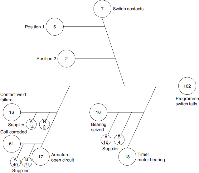
Figure 15.5 Cause and effect diagram.

The cause-and-effect diagram was invented by K. Ishikawa (Ishikawa, 1991) as an aid to structuring and recording problem-solving and process improvement efforts. The diagram is also called a fishbone, or Ishikawa, diagram. The main problem is indicated on a horizontal line, and possible causes are shown as branches, which in turn can have sub-causes, indicated by sub-branches, and so on. An example is shown in Figure 15.5; the numbers in the circles indicate the number of failures attributable to that cause.

15.5.2 Control Charts

When process control charts are in use, they should be monitored continuously for trends that might indicate special causes of variation, so that the causes can be eliminated. Trends can be a continuous run high or low on the chart, or any cyclic pattern. A continuous high or low trend indicates a need for process or measuring adjustment. A cyclic trend might be caused by temperature fluctuations, process drifts between settings, operator changeover, change of material, and so on. Therefore it is important to record supporting data on the SPC chart, such as time and date, to help with the identification of causes. When a process is being run on different machines the SPC charts of the separate processes should be compared, and all statistically significant differences investigated.

15.5.3 Multi-Vari Charts

A multi-vari chart is a graphical method for identifying the major causes of variation in a process. Multi-vari charts can be used for process development and for problem solving, and they can be very effective in reducing the number of variables to include in a statistical experiment.

Multi-vari charts show whether the major causes of variation are spatial, cyclic or temporal. The principle of operation is very simple: the parameter being monitored is measured in different positions (e.g. locations for measurement of a dimension, hardness, etc.), at different points in the production cycle (e.g. batch number from tool change), and at different times. The results are plotted as shown in Figure 15.6, which shows a machined dimension plotted against two measurement locations, for example diameters at each end of a shaft, plotted against batch number from set-up. It shows that batch-to-batch variation is the most significant cause, with a significant pattern of end-to-end variation (taper). This information would then be used to seek the reasons for the major cause, if necessary by running further experiments. Finally, statistical experiments can be run to refine the process further, particularly if interactions are statistically significant. The multi-vari method is described in Bhote (1998).

Figure 15.6 Multi-vari chart.

15.5.4 Statistical Methods

The methods for analysis of variation, described in Chapter 11, can be used just as effectively for variation reduction in production processes. They should be used for process improvement, in the same way as for product and process initial design. If a particular process has been the subject of such experiments during development, then the results can be used to guide studies for further improvement.

The methods described above can also be used to identify the major causes of variation, prior to setting up statistical experiments. In this way the number of variables to be investigated in the statistical experiment can be reduced, leading to cost savings.

15.5.5 ‘Zero Defects’

The ‘zero defects’ (ZD) approach to QC was developed in the United States in the 1960s. ZD is based very much upon setting QC targets, publicizing results and exhortation by award presentations and poster campaigns. Successes were claimed for ZD but it has always been controversial. The motivational basis is evangelical and emotional, and the initial enthusiasm is hard to sustain. There are few managers who can set up and maintain a ZD programme as originally publicized, and consequently the approach is now seldom used.

15.5.6 Quality Circles

The quality circles movement started in Japan in the 1950s, and is now used worldwide. The idea is largely based on Drucker's management teaching, developed and taught for QC application by W. E. Deming and K. Ishikawa. It uses the methods of operator control, consistent with Drucker's teaching that the most effective management is that nearest to the action; this is combined with basic SPC and problem solving methods to identify and correct problems at their sources. The operator is often the person most likely to understand the problems of the process he or she operates, and how to solve them. However, the individual operator does not usually have the authority or the motivation to make changes. Also, he or she might not be able to influence problems elsewhere in the manufacturing system. The quality circles system gives workers this knowledge and influence, by organizing them into small work groups, trained to monitor quality performance, to analyse problems and to recommend solutions to management.

Quality circle teams manage themselves, select their leaders and members, and the problems to be addressed. They introduce the improvements if the methods are under their control. If not, they recommend the solutions to management, who must respond positively.

It is therefore a very different approach to that of ZD, since it introduces quality motivation as a normal working practice at the individual and team level, rather than by exhortation from above. Whilst management must be closely involved and supportive, it does not have to be continually active and visible in the way ZD requires.

Quality circles are taught to use analytical techniques to help to identify problems and generate solutions. These are called the seven tools of quality. The seven tools are:

1. Brainstorm, to identify and prioritize problems.
2. Data collection.
3. Data analysis methods, including measles charts, trend charts and regression analysis.
4. Pareto chart.
5. Histogram.
6. Cause-and-effect (or Ishikawa) diagram.
7. Statistical process control (SPC) chart.

For example, the team would be trained to interpret SPC charts to identify special causes of variation, and to use cause-and-effect diagrams. The cause-and-effect diagram is used by the team leader, usually on a flip chart, to put on view the problem being addressed and the ideas and solutions that are generated by the team, during the ‘brainstorming’ stage.

Quality circles must be organized with care and with the right training, and must have full support from senior and middle management. In particular, quality circles recommendations must be carefully assessed and actioned whenever they will be effective, or good reasons given for not following the recommendation.

The concept is really straightforward, enlightened management applied to the quality control problem, and in retrospect it might seem surprising that it has taken so long to be developed. It has proved to be highly successful in motivating people to produce better quality, and has been part of the foundation of the Japanese industrial revolution since the Second World War. The quality circles approach is closely associated with the concept of kaizen, the Japanese word meaning continuous improvement. The quality circles approach can be very effective when there is no formal quality control organization, for example in a small company.

The quality circles and kaizen approach to quality improvement is described fully in Hutchins (1985) and Imai (1997).

15.6 Quality Control in Electronics Production

15.6.1 Test Methods

Electronic equipment production is characterized by very distinct assembly stages, and specialist test equipment has been developed for each of these. Since electronic production is so ubiquitous, and since test methods can greatly affect quality costs and reliability, it is appropriate to consider test methods for electronics in this context. Test equipment for electronic production falls into the following main categories:

1. Manual test equipment, which includes basic instruments such as digital multimeters (DMMs), oscilloscopes, spectrum analysers, waveform generators, and logic analysers, as well as special instruments, such as radio frequency testers, distortion meters, high voltage testers, optical signal testers, and so on. Computer-based testing uses software that enables PCs to emulate test equipment.
2. Automatic Test Equipment.

Automatic test equipment (ATE) is used for testing manufactured circuits, and also for in-service faultfinding and for testing repaired units. The main types of ATE for assembly testing are:

15.6.1.1 Vision Systems

Vision systems refer generically to inspection systems that acquire an image and then analyse it. They do not actually test circuits, but they have become part of many production test sequences because of the great difficulty of human inspection of the large numbers of components, solder connections and tracks on modern circuits. Automatic optical inspection (AOI) machines are capable of scanning a manufactured circuit and identifying anomalies such as damaged, misplaced or missing components, faulty solder joints, solder spills across conductors, and so on. X-ray systems (AXI) are also used, to enable inspection of otherwise hidden aspects such as solder joints and internal component problems. Other technologies, such as infra-red and laser scanning, are also used.

15.6.1.2 In-Circuit Testers (ICT), Manufacturing Defects Analysers (MDA)

ICT tests the functions of components within circuits, on loaded circuit boards. It does not test the circuit function. The ICT machine accesses the components, one at a time, via a test fixture (sometimes referred to as a ‘bed of nails’ fixture), which consists of a large number of spring loaded contact pins, spaced to make contact with the appropriate test points for each component, for example the two ends of a resistor or the pin connections for an IC. ICT does not test circuit-level aspects such as tolerance mismatch, timing, interference, and so on. MDAs are similar but lower cost machines, with capabilities to detect only manufacturing-induced defects such as opens, shorts, and missing components: justification for their use instead of ICT is the fact that, in most modern electronics assembly, such defects are relatively more common than faulty components. Flying probe testers (also called fixtureless testers) perform the same functions, but access test points on the circuit using probes that are rapidly moved between points, driven by a programmed high-speed positioning system. The advantage over ICT/MDA is the fact that the probe programming is much less expensive and more adaptable to circuit changes than are expensive multipin ICT/MDA adaptors, which must be designed and built for each circuit to be tested. They can also gain access to test points that are difficult to access via a bed-of-nails adaptor.

15.6.1.3 Functional Testers (FT)

Functional testers access the circuit, at the circuit board or assembly level, via the input and output connectors or via a smaller number of spring-loaded probes. They perform a functional test, as driven by the test software. Functional testers usually include facilities for diagnosing the location of causes of incorrect function. There is a wide range, from low-cost bench-top ATE for use in development labs, in relatively low complexity/low production rate manufacture, in-service tests and in repair shops, to very large, high-speed high-capability systems. The modern trend is for production ATE to be specialized, and focused at defined technology areas, such as computing, signal processing, and so on. Some ATE for circuit testing during manufacture includes combined ICT and FT.

Electronics testing is a very fast-moving technology, driven by the advances in circuit performance, packaging and connection technology and production economics. O'Connor (2001) provides an introduction.

It is very important to design circuits to be testable by providing test access points and by including additional circuitry, or it will not be possible to test all functions or to diagnose the causes of certain failures. Design for testability can have a major impact on quality costs and on future maintenance costs. These aspects are covered in more detail in Chapters 9 and 16 and in Davis (1994).

The optimum test strategy for a particular electronic product will depend upon factors such as component quality, quality of the assembly processes, test equipment capability, costs of diagnosis and repair at each stage, and production throughput. Generally, the earlier a defect is detected, the lower will be the cost. A common rule of thumb states that the cost of detecting and correcting a defect increases by a factor of 10 at each test stage (component/PCB, ICT, functional test stages, in-service). Therefore the test strategy must be based on detecting and correcting defects as early as practicable in the production cycle, but defect probability, detection probability and test cost must also be considered.

The many variables involved in electronic equipment testing can be assessed by using computer models of the test options, under the range of assumed input conditions. Figure 15.7 shows a typical test flow arrangement.

Test results must be monitored continuously to ensure that the process is optimized in relation to total costs, including in-service costs. There will inevitably be variation over time. It is important to analyse the causes of failures at later test stages, to determine whether they could have been detected and corrected earlier.

Figure 15.7 Electronic equipment test strategy.

Throughout, the causes of defects must be rapidly detected and eliminated, and this requires a very responsive data collection and analysis system (Section 15.8). Some ATE systems provide data logging and analysis, and data networking between test stations is also available.

Davis (1994) and O'Connor (2001) provide introductions to electronic test methods and economics.

15.6.2 Reliability of Connections

Complete opens and shorts will nearly always be detected during functional test, but open-circuit and intermittent failures can occur in use due to corrosion or fatigue of joints which pass initial visual and functional tests. The main points to watch to ensure solder joint reliability are:

1. Process control. Solder temperature, solder mix (when this is variable, e.g. in wave solder machines), soldering time, fluxes, PCB cleaning.
2. Component mounting. The solder joint should not be used to provide structural support, particularly in equipment subject to vibration or shock, or for components of relatively large mass, such as trimpots and some capacitors.
3. Component preparation. Component connections must be clean and wettable by the solder. Components which have been stored unpackaged for more than a few days or packaged for more than six months require special attention, as oxide formation may inhibit solderability, particularly on automatic soldering systems, where all joints are subject to the same time in the solder wave or oven. If necessary, such components should have their leads cleaned and retinned prior to assembly. Components should be subject to sampling tests for solderability, as near in time to the assembly stage as practicable.
4. Solder joint inspection. Inspectors performing visual inspection of solder joints are typically about 80% effective in seeing joints which do not pass visual inspection standards. Also, it is possible to have unreliable joints which meet appearance criteria. If automatic testing for opens and shorts is used instead of 100% visual inspection, it will not show up marginal joints which can fail later.

Surface mounted devices, as described in Chapter 9, present particular problems, since the solder connections are so much smaller and more closely spaced, and in many cases not visible. Manual soldering is not practicable, so automatic placement and soldering systems must be used. Visual inspection is difficult or impossible, and this has resulted in the development of semi-automatic and automated optical inspection systems, though these cannot be considered to be totally reliable. SMD solderability and soldering must be very carefully controlled to minimize the creation of defective joints.

15.7 Stress Screening

Stress screening, or environmental stress screening (ESS), is the application of stresses that will cause defective production items which pass other tests to fail on test, while not damaging or reducing the useful life of good ones. It is therefore a method for improving reliability and durability in service. Other terms are sometimes used for the process, the commonest being burn-in, particularly for electronic components and systems, for which the stresses usually applied are high temperature and electrical stress (current, voltage). The stress levels and durations to be applied must be determined in relation to the main failure-generating processes and the manufacturing processes that could cause weaknesses. Stress screening is normally a 100% test, that is all manufactured items are tested. Stress screening is applied mainly to electronic components and assemblies, but it should be considered for non-electronic items also, for example precision mechanisms (temperature, vibration) and high pressure tests for pneumatics and hydraulics to check for leaks or other weaknesses.

ESS guidelines have been developed for electronic components and systems. The US Navy has published guidelines (NAVMAT P-9492), and the US DOD published MIL-STD-2164 (ESS Guidelines for Electronics Production), but these were inflexible and the stress levels specified were not severe (typically temperature cycling between 20 and 60 °C for 8 h, with random or fixed frequency vibration in the range 20–2000 Hz, and the equipment not powered or monitored). The US Institute for Environmental Sciences and Technology (IEST) developed more detailed guidelines in 1990 (Environmental Stress Screening of Electronic Hardware (ESSEH)), to cover both development and manufacturing tests. These recommended stress regimes similar to the military ESS guidelines. The details were based to a large extent on industry feedback of the perceived effectiveness of the methods that had been used up to the preparation of the guidelines, so they represented past experience, particularly of military equipment manufacture.

If ESS shows up very few defects, it is either insufficiently severe or the product being screened is already highly reliable. Obviously the latter situation is preferable, and all failures during screening should be analysed to determine if QC methods should have prevented them or discovered them earlier, particularly prior to assembly. At this stage, repairs are expensive, so eliminating the need for them by using high quality components and processes during production is a worthwhile objective.

Screening is expensive, so its application must be carefully monitored. Failure data should be analysed continuously to enable the process to be optimized in terms of operating conditions and duration. Times between failures should be logged to enable the process to be optimized.

Screening must be considered in the development of the production test strategy. The costs and effects in terms of reduced failure costs in service and the relationships with other test methods and QC methods must be assessed as part of the integrated quality assurance approach. Much depends upon the reliability requirement and the costs of failures in service. Also, screening should ensure that manufacturing quality problems are detected before shipment, so that they can be corrected before they affect much production output. With large-scale production, particularly of commercial and domestic equipment, screening of samples is sometimes applied for this purpose.

Jensen and Peterson (1983) describe methods and analytical techniques for screening of electronic components and assemblies.

15.7.1 Highly Accelerated Stress Screening

Highly accelerated stress screening (HASS) is an extension of the HALT principle, as described in Chapter 12, that makes use of very high combined stresses. No ‘guidelines’ are published to recommend particular stresses and durations. Instead, the stresses, cycles and durations are determined separately for each product (or group of similar products) by applying HALT during development. HALT shows up the product weak points, which are then strengthened as far as practicable so that failures will occur only well beyond the envelope of expected in-service combined stresses. The stresses that are then applied during HASS are higher than the operating limit, and extend into the lower tail of the distribution of the permanent failure limit. It is essential that the equipment under test is operated and monitored throughout.

The stresses applied in HASS, like those applied in HALT, are not designed to represent worst-case service conditions. They are designed to precipitate failures which would otherwise occur in service. This is why they can be developed only by applying HALT in development, and why they must be specific to each product design. Because the stress levels are so high, they cannot be applied safely to any design that has not been ruggedized through HALT.

Obviously the determination of this stress–time combination cannot be exact, because of the uncertainty inherent in the distribution of strength. However, by exploring the product's behaviour on test, we can determine appropriate stress levels and durations. The durations will be short, since the stress application rates are very high and there is usually no benefit to be gained by, for example, operating at constant high or low temperatures for longer than it takes for them to stabilize. Also, only a few stress cycles will be necessary, typically one to four.

When stresses above the operating limit are applied, it will not be possible to perform functional tests. Therefore the stresses must then be reduced to levels below the operating limit. The functional test will then show which items have been caused to fail, and which have survived. The screening process is therefore in two stages: the precipitation screen followed by the detection screen, as shown in Figure 15.8.

The total test time for HASS is much less than for conventional ESS: a few minutes vs. many hours. HASS is also much more effective at detecting defects. Therefore it is far more cost effective, by orders of magnitude. HASS is applied using the same facilities, particularly environmental chambers, as used for HALT. Since the test times are so short, it is often convenient to use the same facilities during development and in production, leading to further savings in relation to test and monitoring equipment, interfaces, and so on. The HASS concept can be applied to any type of product or technology. It is by no means limited to electronic assemblies. If the design can be improved by HALT, as described in Chapter 12, then in principle manufacturing quality can be improved by HASS. The HASS approach to manufacturing stress screening is described fully in McLean (2009).

Figure 15.8 HASS.

15.8 Production Failure Reporting Analysis and Corrective Action System (FRACAS)

Failure reporting and analysis is an important part of the QA function. The system must provide for:

1. Reporting of all production test and inspection failures with sufficient detail to enable investigation and corrective action to be taken.
2. Reporting the results of investigation and action.
3. Analysis of failure patterns and trends, and reporting on these.
4. Continuous improvement (kaizen) by removal of causes of failures.

The FRACAS principles (Section 12.6) are equally applicable to production failures.

The data system should be computerized for economy and accuracy. Modern ATE sometimes includes direct test data recording and inputting to a central system by networking. The data analysis system should provide Pareto analysis, probability plots and trend analyses for management reporting.

Production defect data reporting and analysis must be very quick to be effective. Trends should be analysed daily, or weekly at most, particularly for high rates of production, to enable timely corrective action to be taken. Production problems usually arise quickly, and the system must be able to detect a bad batch of components or an improperly adjusted process as soon as possible. Many problems become immediately apparent without the aid of a data analysis system, but a change of, say, 50% in the proportion of a particular component in a system failing on test might not be noticed otherwise. The data analysis system is also necessary for indicating areas for priority action, using the Pareto principle of concentrating action on the few problem areas that contribute the most to quality costs. For this purpose longer term analysis, say monthly, is necessary.

Defective components should not be scrapped immediately, but should be labelled and stored for a period, say one to two months, so that they are available for more detailed investigation if necessary.

Production defect data should not be analysed in isolation by people whose task is primarily data management. The people involved (production, supervisors, QC engineers, test operators, etc.) must participate to ensure that the data are interpreted by those involved and that practical results are derived. The quality circles approach provides very effectively for this.

Production defect data are important for highlighting possible in-service reliability problems. Many inservice failure modes manifest themselves during production inspection and test. For example, if a component or process generates failures on the final functional test, and these are corrected before delivery, it is possible that the failure mechanism exists in products which pass test and are shipped. Metal surface protection and soldering processes present such risks, as can almost any component in electronic production. Therefore production defects should always be analysed to determine the likely effects on reliability and on external failure costs, as well as on internal production quality costs.

15.9 Conclusions

The modern approach to production quality control and improvement is based on the use of statistical methods and on organizing, motivating and training production people at all levels to work for continuously improving performance, of people and of processes. A very close link must exist between design and development of the product and of the production processes, and the criteria and methods to be used to control the processes. This integrated approach to management of the design and production processes is described in more detail in Chapter 17. The journals of the main professional societies for quality (see the Bibliography) also provide information on new developments.

Questions

1. A machined dimension on a component is specified as 12.50 mm ± 0.10 mm. A preliminary series of ten samples, each of five components, is taken from the process, with measurements of the dimension as follows:

   

   1. Use the averages and ranges for each sample to assess the capability of the process (calculated C_p and C_pk).
   2. Use the relationship (taken from BS 5700) that, for samples of size 5, standard deviation = average range × 2.326.
   3. Suggest any action that may be necessary.
2. Sketch the two charts used for statistical process control. What is the primary objective of the method?
3. Explain why statistical acceptance sampling is not an effective method for monitoring processes quality.
4. A particular component is used in large quantities in an assembly. It costs very little, but some protection against defective components is needed as they can be easily detected only after they have been built-in to an expensive assembly, which is then scrap if it contains a defective component. 100% inspection of the components is not possible as testing at the component level would be destructive, but the idea of acceptance sampling is attractive.
   1. How would you decide on the AQL to use?
   2. If the AQL was 0.4% defective and these components were supplied in batches of 2500, what sampling plan would you select from Table 15.1? (Batches of 2500 require sample size code K for general inspection, level II.)
   3. What would you do if you detected a single defective component in the sample?
   4. What would you do if this plan caused a batch to be rejected?
5. A manufacturing line produces car radios. The cost of the final test is $; 15, and the average proportion found to be not working is 0.007, though on some batches it is as high as 0.02. If the total cost of selling a non-working radio (replacement, administration, etc.) is $ 400, comment on the continued application of the test.
6. List the ‘7 tools of quality’ as applied in the Quality Circles approach. Explain how they are applied by a Quality Circles team.
7. Briefly describe the three main approaches used for automatic inspection and test of modern electronic circuits. Sketch a typical inspection/test flow for a line producing circuit assemblies.
8. Describe the stresses that are typically applied to electronic hardware during environmental stress screening (ESS) in manufacturing.
9. 1. Define the main advantages and disadvantages of applying environmental stress screening (ESS) to electronic assemblies in production.
   2. Discuss why it would be wrong to impose an ESS using MIL-HDBK-781 type environmental profiles.
10. How does highly accelerated stress screening (HASS) differ from conventional ESS? How is it related to HALT in development?
11. 1. Explain the difference between reducing failure rate by ‘burn-in’ and by reliability growth in service.
    2. Assuming that you are responsible for the reliability of a complex electronic system, that is about to go into production, outline the way that you would set up ‘burn-in’ testing for purchased components, sub-assemblies and the completed product, in each case stating the purpose of the test and the criteria you would consider in deciding its duration.
12. What would be the C_p and C_pk values for a ‘6-sigma process’, which shifts ±1.5σ?
13. As mentioned at the beginning of Section 15.2, SPC is based on the assumption that the process follows the normal distribution, which sometimes is not the case. How would you analyse a process which can be modelled by a skewed distribution, for example lognormal?
14. Compare the Fault Tree Analysis and the Ishikawa diagram methods. What are the similarities and the differences of the two methods?

Bibliography

ANSI/ASQ Z1–4. Sampling Procedures and Tables for Inspection by Attributes.

Bergman B. and Klefsjö, B. (2003) Quality: from Customer Needs to Customer Satisfaction, 3rd edn, McGraw-Hill.

Bhote, K.R. (1998) World Class Quality, American Management Association.

British Standard BS 6001. Sampling Procedures and Tables for Inspection by Attributes.

Davis, B. (1994) The Economics of Automatic Test Equipment, 2nd edn, McGraw-Hill.

Defeo, J. and Juran, J. (2010) Juran's Quality Handbook, 6th. edn, McGraw-Hill.

Deming, W.E. (1987) Out of the Crisis, MIT University Press.

Feigenbaum, A.V. (1991) Total Quality Control, 3rd edn, McGraw-Hill.

Grant, E.L. and Leavenworth, R.S. (1996) Statistical Quality Control, 6th edn, McGraw-Hill.

Hutchins, D.C. (1985) Quality Circles Handbook. Pitman.

Imai, M. (1997) Gemba Kaizen. McGraw-Hill.

Ishikawa, K. (1991) Guide to Quality Control. Chapman and Hall.

Jensen, F., Peterson, N.E. (1983) Burn-in: An Engineering Approach to the Design and Analysis of Burn-in Procedures. Wiley.

McLean, H. (2009) Halt, Hass, and Hasa Explained: Accelerated Reliability Techniques, American Society for Quality (ASQ) Publishing.

Montgomery, D.C. (2008) Introduction to Statistical Quality Control, Wiley.

Oakland, J.S. and Followell, R.F. (2003) Statistical Process Control, a Practical Guide, 5th edn, Butterworth-Heinemann.

O'Connor, P.D.T. (2001) Test Engineering, Wiley.

Quality Assurance. Journal of the Institute of Quality Assurance (UK).

Quality Progress. Journal of the American Society for Quality.

Thomas, B. (1995) The Human Dimension of Quality, McGraw-Hill.