
Chapter 3
Sampling Rate Conversion
U. Zölzer
Several different sampling rates are established for digital audio applications. For broadcasting, professional, and consumer audio, sampling rates of 32, 48, and 44.1 kHz are used, respectively. Moreover, other sampling rates are derived from different frame rates for film and video. In connecting systems with different uncoupled sampling rates, there is a need for sampling rate conversion. In this chapter, synchronous sampling rate conversion with rational factor ![]() for coupled clock rates and asynchronous sampling rate conversion will be discussed where the different sampling rates are not synchronized with each other.
for coupled clock rates and asynchronous sampling rate conversion will be discussed where the different sampling rates are not synchronized with each other.
3.1 Basics
Sampling rate conversion consists of upsampling and downsampling and anti‐imaging and antialiasing filtering [Cro83, Vai93, Fli00, Opp99]. The discrete‐time Fourier transform of the sampled signal ![]() with sampling frequency
with sampling frequency ![]() (
(![]() ) is given by
) is given by

with the Fourier transform ![]() of the continuous‐time signal
of the continuous‐time signal ![]() . For ideal sampling, the condition
. For ideal sampling, the condition
holds.
3.1.1 Upsampling and Anti‐Imaging Filtering
For upsampling, the signal
by factor ![]() between consecutive samples
between consecutive samples ![]() , zero samples will be included (see Fig. 3.1). This leads to the upsampled signal
, zero samples will be included (see Fig. 3.1). This leads to the upsampled signal

with sampling frequency ![]() (
(![]() ) and the corresponding Fourier transform
) and the corresponding Fourier transform
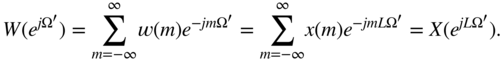
The suppression of the image spectra is achieved by anti‐imaging filtering of ![]() with
with ![]() , such that the output signal is given by
, such that the output signal is given by
For adjusting the signal power in the baseband, the Fourier transform of the impulse response
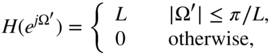
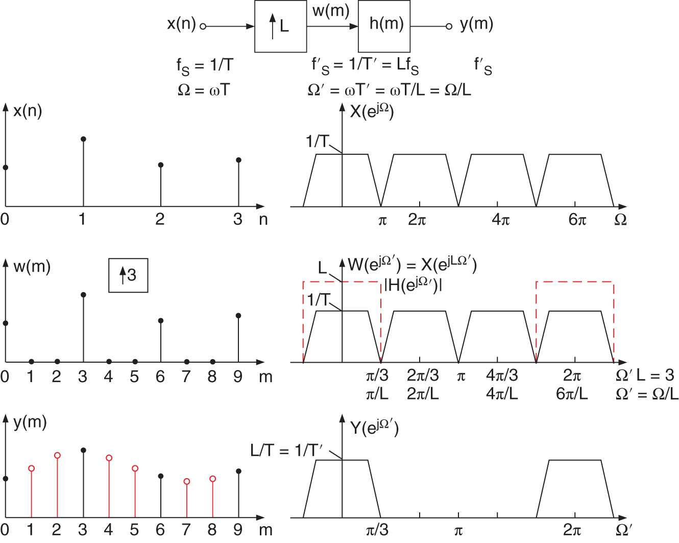
Figure 3.1 Upsampling by L and anti‐imaging filtering in the time and frequency domains.
needs a gain factor ![]() in the passband, such that the output signal
in the passband, such that the output signal ![]() has the Fourier transform given by
has the Fourier transform given by
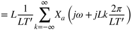

The output signal represents the sampling of the input ![]() with sampling frequency
with sampling frequency ![]() .
.
3.1.2 Downsampling and Antialiasing Filtering
For downsampling a signal ![]() by
by ![]() , the signal has to be band limited to
, the signal has to be band limited to ![]() to avoid aliasing after the downsampling operation (see Fig. 3.2). Band limiting is achieved by filtering with
to avoid aliasing after the downsampling operation (see Fig. 3.2). Band limiting is achieved by filtering with ![]() according to
according to

Downsampling of ![]() is performed by taking every
is performed by taking every ![]() th sample, which leads to the output signal
th sample, which leads to the output signal
with the Fourier transform
For the baseband spectrum (![]() and
and ![]() ), we get
), we get
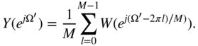
and for the Fourier transform of the output signal, we can derive


Figure 3.2 Antialiasing filtering and downsampling by M in the time and frequency domains.

which represents a sampled signal ![]() with
with ![]() .
.
3.2 Synchronous Conversion
Sampling rate conversion for coupled sampling rates by a rational factor ![]() can be performed by the system shown in Fig. 3.3. After upsampling by a factor
can be performed by the system shown in Fig. 3.3. After upsampling by a factor ![]() , anti‐imaging filtering at
, anti‐imaging filtering at ![]() is done followed by downsampling by factor
is done followed by downsampling by factor ![]() . Because after upsampling and filtering only every
. Because after upsampling and filtering only every ![]() th sample is used, it is possible to develop efficient algorithms that reduce the complexity. In this respect, two methods are in use; one is based on a time‐domain interpretation [Cro83] and the other [Hsi87] uses Z‐domain fundamentals. Owing to its computational efficiency, only the method in the Z‐domain will be considered.
th sample is used, it is possible to develop efficient algorithms that reduce the complexity. In this respect, two methods are in use; one is based on a time‐domain interpretation [Cro83] and the other [Hsi87] uses Z‐domain fundamentals. Owing to its computational efficiency, only the method in the Z‐domain will be considered.

Figure 3.3 Sampling rate conversion by factor L/M.
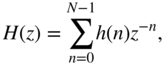
Starting with the finite impulse response ![]() of length
of length ![]() and its Z‐transform
and its Z‐transform
the polyphase representation [Cro83, Vai93, Fli00] with ![]() components can be expressed as
components can be expressed as
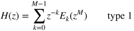
or
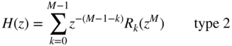
The polyphase decomposition as given in Eqs. (3.22) and (3.24) is denoted as type 1 and 2, respectively. The type‐1 polyphase decomposition corresponds to a commutator model in the anticlockwise direction, whereas the type 2 is in the clockwise direction. The relationship between ![]() and
and ![]() is described by
is described by
With the help of the identities [Vai93] shown in Fig. 3.4 and the decomposition (Euclid's theorem)
it is possible to move the inner delay elements of Fig. 3.5. Equation (3.27) is valid if ![]() and
and ![]() are prime numbers. In a cascade of upsampling and downsampling, the order of functional blocks can be exchanged (see Fig. 3.5b).
are prime numbers. In a cascade of upsampling and downsampling, the order of functional blocks can be exchanged (see Fig. 3.5b).
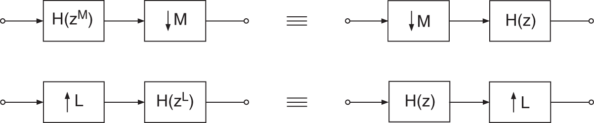
Figure 3.4 Identities for sampling rate conversion.
The use of polyphase decomposition can be demonstrated with the help of an example for ![]() and
and ![]() . This implies a sampling rate conversion from 48 kHz to 32 kHz. Figures 3.6 and 3.7 show two different solutions for polyphase decomposition of sampling rate conversion by
. This implies a sampling rate conversion from 48 kHz to 32 kHz. Figures 3.6 and 3.7 show two different solutions for polyphase decomposition of sampling rate conversion by ![]() . Further decompositions of the upsampling decomposition of Fig. 3.7 are demonstrated in Fig. 3.8. First, interpolation is implemented with a polyphase decomposition and the delay
. Further decompositions of the upsampling decomposition of Fig. 3.7 are demonstrated in Fig. 3.8. First, interpolation is implemented with a polyphase decomposition and the delay ![]() is decomposed to
is decomposed to ![]() . Then, the downsampler of factor 3 is moved through the adder into the two paths (Fig. 3.8b) and the delays are moved according to the identities of Fig. 3.4. In Fig. 3.8c, the upsampler is exchanged with the downsampler and in a last step (Fig. 3.8d), another polyphase decomposition of
. Then, the downsampler of factor 3 is moved through the adder into the two paths (Fig. 3.8b) and the delays are moved according to the identities of Fig. 3.4. In Fig. 3.8c, the upsampler is exchanged with the downsampler and in a last step (Fig. 3.8d), another polyphase decomposition of ![]() and
and ![]() is carried out. The actual filter operations
is carried out. The actual filter operations ![]() and
and ![]() with
with ![]() are performed at
are performed at ![]() of the input sampling rate.
of the input sampling rate.

Figure 3.5 Decomposition in accordance with Euclid's theorem.

Figure 3.6 Polyphase decomposition for downsampling L/M .
.

Figure 3.7 Polyphase decomposition for upsampling L/M .
.

Figure 3.8 Sampling rate conversion by factor  .
.
3.3 Asynchronous Conversion
Plesiochronous systems consist of partial systems with different and uncoupled sampling rates. Sampling rate conversion between such systems can be achieved through a DA conversion with the sampling rate of the first system followed by an AD conversion with the sampling rate of the second system. A digital approximation of this approach is made with a multi‐rate system [Lag81, Lag82a, Lag82b, Lag82c, Lag83, Ram82, Ram84]. Figure 3.9a shows a system for increasing the sampling rate by a factor ![]() followed by an anti‐imaging filter
followed by an anti‐imaging filter ![]() and a resampling of the interpolated signal
and a resampling of the interpolated signal ![]() . The samples
. The samples ![]() are held for a clock period (see Fig. 3.9c) and then sampled with output clock period
are held for a clock period (see Fig. 3.9c) and then sampled with output clock period ![]() . The interpolation sampling rate must be increased so that the difference of two consecutive samples
. The interpolation sampling rate must be increased so that the difference of two consecutive samples ![]() is smaller than the quantization step
is smaller than the quantization step ![]() . The sample‐and‐hold function applied to
. The sample‐and‐hold function applied to ![]() suppresses the spectral images at multiples of
suppresses the spectral images at multiples of ![]() (see Fig. 3.9b). The obtained signal is a band‐limited continuous‐time signal which can be sampled with output sampling rate
(see Fig. 3.9b). The obtained signal is a band‐limited continuous‐time signal which can be sampled with output sampling rate ![]() .
.
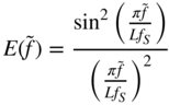
For the calculation of the necessary oversampling rate, the problem is considered in the frequency domain. The sinc function of a sample‐and‐hold system (see Fig. 3.9b) at frequency ![]() is given by
is given by
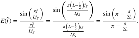

Figure 3.9 Approximation of DA/AD conversions.
With ![]() , we derive
, we derive
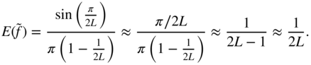
This value of Eq. (3.29) should be lower than ![]() and allows the computation of the interpolation factor
and allows the computation of the interpolation factor ![]() . For a given word length
. For a given word length ![]() and quantization step
and quantization step ![]() , the necessary interpolation rate
, the necessary interpolation rate ![]() is calculated by
is calculated by

For a linear interpolation between upsampled samples ![]() , we can derive
, we can derive


With this, it is possible to reduce the necessary interpolation rate to
Figure (3.10) demonstrates this with a two‐stage block diagram. First, interpolation up to a sampling rate ![]() is performed by conventional filtering. In the second stage, upsampling by factor
is performed by conventional filtering. In the second stage, upsampling by factor ![]() is done by linear interpolation. The two‐stage approach must satisfy the sampling rate
is done by linear interpolation. The two‐stage approach must satisfy the sampling rate ![]() .
.

Figure 3.10 Linear interpolation before virtual sample‐and‐hold function.
The choice of the interpolation algorithm in the second stage enables the reduction of the first oversampling factor.
3.3.1 Single‐stage Methods
Direct conversion methods implement the block diagram [Lag83, Smi84, Par90, Par91a, Par91b, Ada92, Ada93] shown in Fig. 3.9a. The calculation of a discrete sample on an output grid of sampling rate ![]() from samples
from samples ![]() at sampling rate
at sampling rate ![]() can be written as
can be written as

where ![]() . With the transfer function
. With the transfer function
and the properties

the impulse response is given by

From Eq. (3.37), we can express the delayed signal


as the convolution between ![]() and
and ![]() . Figure 3.11 illustrates this convolution in the time domain for a fixed
. Figure 3.11 illustrates this convolution in the time domain for a fixed ![]() . Fig. 3.12 shows the coefficients
. Fig. 3.12 shows the coefficients ![]() for discrete
for discrete ![]() (
(![]() ) which are obtained from the intersection of the sinc function with the discrete samples
) which are obtained from the intersection of the sinc function with the discrete samples ![]() .
.
To limit the convolution sum, the impulse response is windowed, which gives
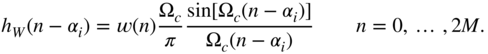

Figure 3.11 Convolution sum (3.42) in the time domain.
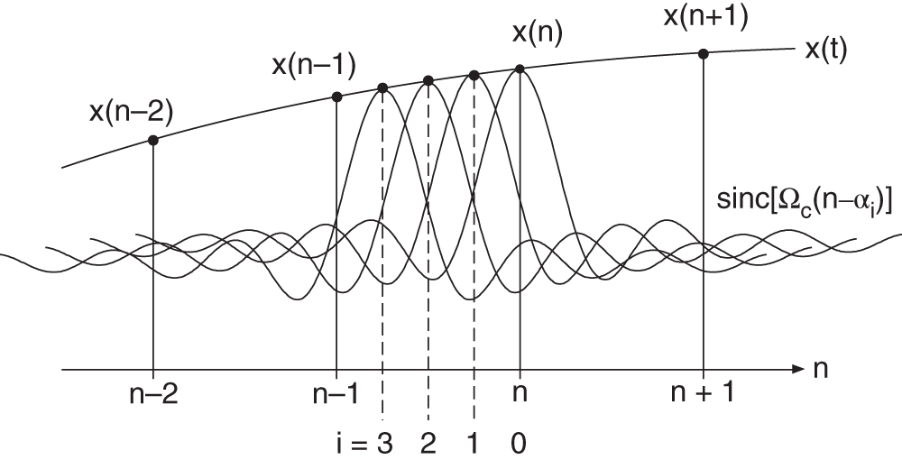
Figure 3.12 Convolution sum (3.42) for different  .
.
From this, the sample estimate

results. A graphical interpretation of the time‐variant impulse response which depends on ![]() is shown in Fig. 3.13. The discrete segmentation between two input samples into
is shown in Fig. 3.13. The discrete segmentation between two input samples into ![]() intervals leads to
intervals leads to ![]() partial impulse responses of length
partial impulse responses of length ![]() .
.

Figure 3.13 Sinc function and different impulse responses.
If the output sampling rate is smaller than the input sampling rate (![]() ), band limiting (antialiasing) to the output sampling rate has to be done. This can be achieved with factor
), band limiting (antialiasing) to the output sampling rate has to be done. This can be achieved with factor ![]() and leads, with the the scaling theorem of the Fourier transform, to
and leads, with the the scaling theorem of the Fourier transform, to

This time scaling of the impulse response has the consequence that the number of coefficients of the time‐variant partial impulse responses is increased. The number of required states also increases. Figure 3.14 shows the time‐scaled impulse response and elucidates the increase of the number ![]() of the coefficients.
of the coefficients.
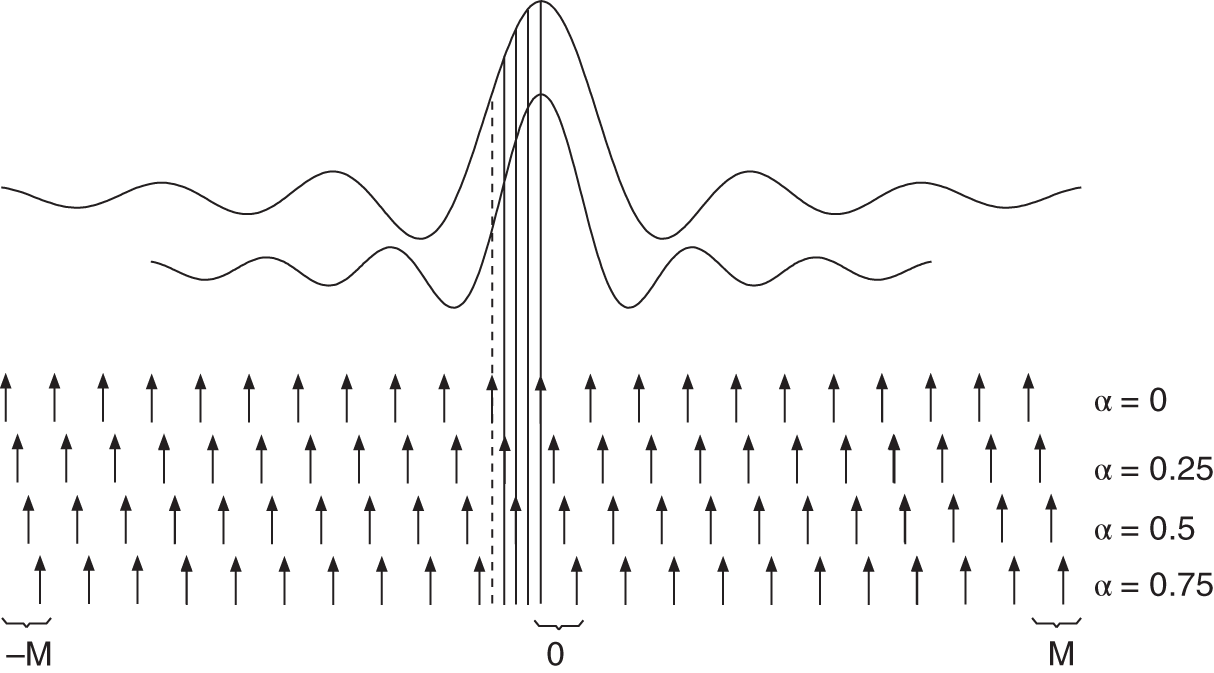
Figure 3.14 Time‐scaled impulse response.
3.3.2 Multistage Methods
The basis of a multistage conversion method [Lag81, Lag82a, Lag82b, Lag82c, Kat85, Kat86] is shown in Fig. 3.15a and will be described in the frequency domain, as shown in Fig. 3.15b–d. The increase of the sampling rate up to the rate ![]() before the sample‐and‐hold function is done in four stages. In the first two stages, the sampling rate is increased by a factor of two followed by an anti‐imaging filter (see Fig. 3.15b,c), which leads to a four‐times oversampled spectrum (Fig. 3.15d). In the third stage, the signal is upsampled by a factor of 32 and the image spectra are suppressed (see Fig. 3.15d,e). In the fourth stage (Fig. 3.15e), the signal is upsampled to a sampling rate of
before the sample‐and‐hold function is done in four stages. In the first two stages, the sampling rate is increased by a factor of two followed by an anti‐imaging filter (see Fig. 3.15b,c), which leads to a four‐times oversampled spectrum (Fig. 3.15d). In the third stage, the signal is upsampled by a factor of 32 and the image spectra are suppressed (see Fig. 3.15d,e). In the fourth stage (Fig. 3.15e), the signal is upsampled to a sampling rate of ![]() by a factor of 256 and a linear interpolator. The
by a factor of 256 and a linear interpolator. The ![]() ‐function of the linear interpolator suppresses the images at multiples of
‐function of the linear interpolator suppresses the images at multiples of ![]() up to the spectrum at
up to the spectrum at ![]() . The virtual sample‐and‐hold function is shown in Fig. 3.15f, where resampling at the output sampling rate is performed. A direct conversion of this kind of cascaded interpolation structure requires anti‐imaging filtering after every upsampling with the corresponding sampling rate. Although the necessary filter order decreases owing to a decrease of requirements for filter design, an implementation of the filters in the third and fourth stages is not possible directly. After a suggestion by Lagadec [Lag82c], the measurement of the ratio of input to output rate is used to control the polyphase filters in the third and fourth stages (see Fig. 3.16a, CON = control) to reduce complexity. Figure 3.16b–d illustrate an interpretation in the time domain. Figure 3.16b shows the interpolation of three samples between two input samples
. The virtual sample‐and‐hold function is shown in Fig. 3.15f, where resampling at the output sampling rate is performed. A direct conversion of this kind of cascaded interpolation structure requires anti‐imaging filtering after every upsampling with the corresponding sampling rate. Although the necessary filter order decreases owing to a decrease of requirements for filter design, an implementation of the filters in the third and fourth stages is not possible directly. After a suggestion by Lagadec [Lag82c], the measurement of the ratio of input to output rate is used to control the polyphase filters in the third and fourth stages (see Fig. 3.16a, CON = control) to reduce complexity. Figure 3.16b–d illustrate an interpretation in the time domain. Figure 3.16b shows the interpolation of three samples between two input samples ![]() with the help of the first and second interpolation stages. The abscissa represents the intervals of the input sampling rate and the sampling rate is increased by a factor of four. In Fig. 3.16c, the four‐times oversampled signal is shown. The abscissa shows the four‐ times oversampled output grid. It is assumed that the output sample
with the help of the first and second interpolation stages. The abscissa represents the intervals of the input sampling rate and the sampling rate is increased by a factor of four. In Fig. 3.16c, the four‐times oversampled signal is shown. The abscissa shows the four‐ times oversampled output grid. It is assumed that the output sample ![]() and input sample
and input sample ![]() are identical. The output sample
are identical. The output sample ![]() is now determined in such a form that, with the interpolator in the third stage, only two polyphase filters just before and after the output sample need to be calculated. Hence, only two out of a total of 31 possible polyphase filters are calculated in the third stage. Fig. 3.16d shows these two polyphase output samples. Between these two samples, the output sample
is now determined in such a form that, with the interpolator in the third stage, only two polyphase filters just before and after the output sample need to be calculated. Hence, only two out of a total of 31 possible polyphase filters are calculated in the third stage. Fig. 3.16d shows these two polyphase output samples. Between these two samples, the output sample ![]() is obtained with a linear interpolation on a grid of 255 values.
is obtained with a linear interpolation on a grid of 255 values.

Figure 3.15 Multistage conversion – frequency‐domain interpretation.
Instead of the third and fourth stages, special interpolation methods can be used to calculate the output ![]() directly from the four‐times oversampled input signal (see Fig. 3.17) [Sti91, Cuc91, Liu92]. The upsampling factor
directly from the four‐times oversampled input signal (see Fig. 3.17) [Sti91, Cuc91, Liu92]. The upsampling factor ![]() for the last stage is calculated according to
for the last stage is calculated according to ![]() . Section 3.4 is devoted to different interpolation methods which allow a real‐time calculation of filter coefficients. This can be interpreted as time‐variant filters in which the filter coefficients are derived from the ratio of sampling rates. The calculation of one filter coefficient set for the output sample at the output rate is done by measuring the ratio of input to output sampling rate as described in the next section.
. Section 3.4 is devoted to different interpolation methods which allow a real‐time calculation of filter coefficients. This can be interpreted as time‐variant filters in which the filter coefficients are derived from the ratio of sampling rates. The calculation of one filter coefficient set for the output sample at the output rate is done by measuring the ratio of input to output sampling rate as described in the next section.
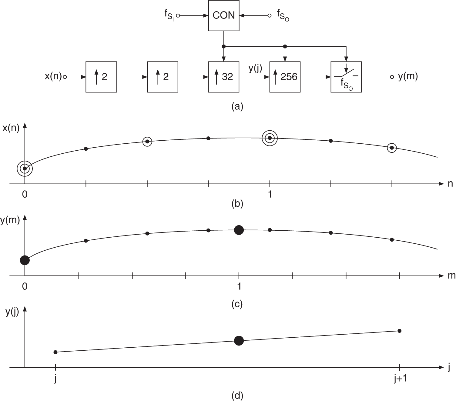
Figure 3.16 Time‐domain interpretation.
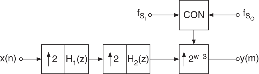
Figure 3.17 Sampling rate conversion with interpolation for calculating coefficients of a time‐variant interpolation filter.
3.3.3 Control of Interpolation Filters
The measurement of the ratio of input and output sampling rates is used to control the interpolation filters [Lag82a]. By increasing the sampling rate by a factor of ![]() , the input sampling period is divided into
, the input sampling period is divided into ![]() parts for a signal word‐length of
parts for a signal word‐length of ![]() bits. The time instant of the output sample is calculated on this grid with the help of the measured ratio of sampling periods
bits. The time instant of the output sample is calculated on this grid with the help of the measured ratio of sampling periods ![]() as follows.
as follows.
A counter is clocked with ![]() and reset by every new input sampling clock. A sawtooth curve of the counter output versus time is obtained, as shown in Fig. 3.18. The counter runs from 0 to
and reset by every new input sampling clock. A sawtooth curve of the counter output versus time is obtained, as shown in Fig. 3.18. The counter runs from 0 to ![]() during one input sampling period. At time
during one input sampling period. At time ![]() , which corresponds to counter output
, which corresponds to counter output ![]() , the output sampling period
, the output sampling period ![]() starts, and stops at time
starts, and stops at time ![]() with counter output
with counter output ![]() . The difference between both counter measurements allows for the calculation of the output sampling period
. The difference between both counter measurements allows for the calculation of the output sampling period ![]() with a resolution of
with a resolution of ![]() .
.

Figure 3.18 Calculation of  .
.
The new counter measurement is added to the difference of the previous counter measurements. As a result, the new counter measurement is obtained as
The modulo operation can be carried out with an accumulator of word length ![]() . The resulting time
. The resulting time ![]() determines the time instant of the output sample at the output sampling rate and therefore the choice of the polyphase filter in a single‐stage conversion or the time instant for a multistage conversion.
determines the time instant of the output sample at the output sampling rate and therefore the choice of the polyphase filter in a single‐stage conversion or the time instant for a multistage conversion.
The measurement of ![]() is illustrated in Fig. 3.19.
is illustrated in Fig. 3.19.
- The input sampling rate
 is increased to
  using a frequency multiplier, where
  . This increased input clock by the factor
  triggers a
  ‐bit counter. The counter output
  is evaluated every
  output sampling periods.
 - Counting of
 output sampling periods.
 - Simultaneous counting of the
 input sampling periods.
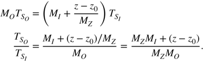
The time intervals ![]() and
and ![]() (see Fig. 3.19) are given by
(see Fig. 3.19) are given by

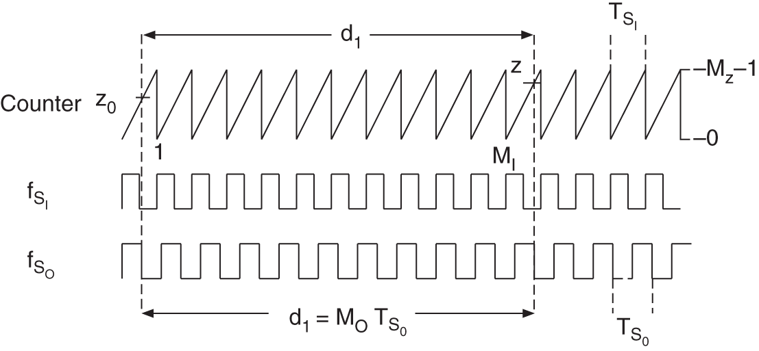
Figure 3.19 Measurement of  .
.
and with the requirement ![]() , we can write
, we can write
- Example 1:
 ,
(3.50)
,
(3.50)
With a precision of 15 bits, the averaging number is chosen as
 and the number
  has to be determined.
 - Example 2:
 ,
(3.51)
,
(3.51)
With a precision of 15 bits, the averaging number is chosen as
 and the number
  , as well as the counter outputs, has to be determined.
The sampling rates at the input and output of a sampling rate converter can be calculated by evaluating the 8‐bit increment of the counter for each output clock with
as seen from Table 3.1.
Table 3.1 Counter increments for different sampling rate conversions.
| Conversion/kHz | 8‐bit counter increment | ||
|---|---|---|---|
| 32 | 48 | 170 | |
| 44.1 | 48 | 235 | |
| 32 | 44.1 | 185 | |
| 48 | 44.1 | 278 | |
| 48 | 32 | 384 | |
| 44.1 | 32 | 352 | |
3.4 Interpolation Methods
In the following sections, special interpolation methods are discussed. These methods enable the calculation of time‐variant filter coefficients for sampling rate conversion and need an oversampled input sequence as well as the time instant of the output sample. A convolution of the oversampled input sequence with time‐variant filter coefficients gives the output sample at the output sampling rate. This real‐time computation of filter coefficients is not based on popular filter design methods. On the contrary, methods are presented for calculating filter coefficient sets for every input clock cycle where the filter coefficients are derived from the distance of output samples to the time grid of the oversampled input sequence.
3.4.1 Polynomial Interpolation
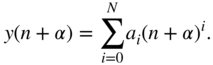
The aim of a polynomial interpolation [Liu92] is to determine a polynomial

of ![]() th order representing exactly a function
th order representing exactly a function ![]() at
at ![]() uniformly spaced
uniformly spaced ![]() , i.e.
, i.e. ![]() for
for ![]() . This can be written as a set of linear equations:
. This can be written as a set of linear equations:

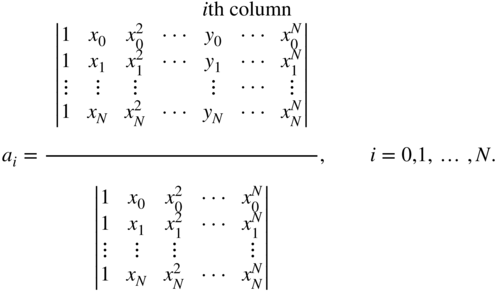
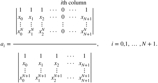
The polynomial coefficients ![]() as functions of
as functions of ![]() are obtained with the help of Cramer's Rule according to
are obtained with the help of Cramer's Rule according to
For uniformly spaced ![]() with
with ![]() , the interpolation of an output sample with distance
, the interpolation of an output sample with distance ![]() gives
gives
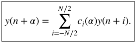
To determine the relationship between the output sample ![]() and
and ![]() , a set of time‐variant coefficients
, a set of time‐variant coefficients ![]() needs to be determined such that
needs to be determined such that
The calculation of time‐variant coefficients ![]() will be illustrated by an example.
will be illustrated by an example.
3.4.2 Lagrange Interpolation
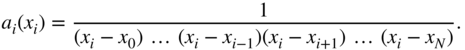
Lagrange interpolation for ![]() samples makes use of the polynomials
samples makes use of the polynomials ![]() which have the following properties (see Fig. 3.21):
which have the following properties (see Fig. 3.21):


Figure 3.21 Lagrange polynomial.
Based on the zeros of the polynomial ![]() , it follows that
, it follows that
With ![]() , the coefficients are given by
, the coefficients are given by
The interpolation polynomial is expressed as

With ![]() , Eq. (3.66) can be written as
, Eq. (3.66) can be written as

For uniformly spaced samples,
and with the new variable ![]() , as given by
, as given by
we get

and hence

For even ![]() , we can write
, we can write

and for odd ![]() ,
,

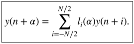
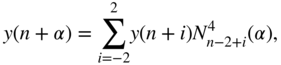
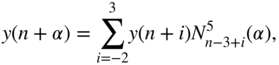
The interpolation of an output sample is given by
3.4.3 Spline Interpolation
The interpolation using piecewise‐defined functions that only exist over finite intervals is called spline interpolation [Cuc91]. The goal is to compute the sample ![]() from weighted samples
from weighted samples ![]() .
.
A B‐spline ![]() of
of ![]() th order using
th order using ![]() samples is defined in the interval
samples is defined in the interval ![]() by
by

with the truncated power functions

In the following, ![]() will be considered for
will be considered for ![]() , where
, where ![]() for
for ![]() and
and ![]() for
for ![]() . Figure 3.22 shows the truncated power functions and the B‐spline of
. Figure 3.22 shows the truncated power functions and the B‐spline of ![]() th order. With the definition of the truncated power functions, we can write
th order. With the definition of the truncated power functions, we can write

and after some calculations, we get
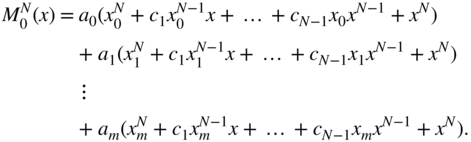
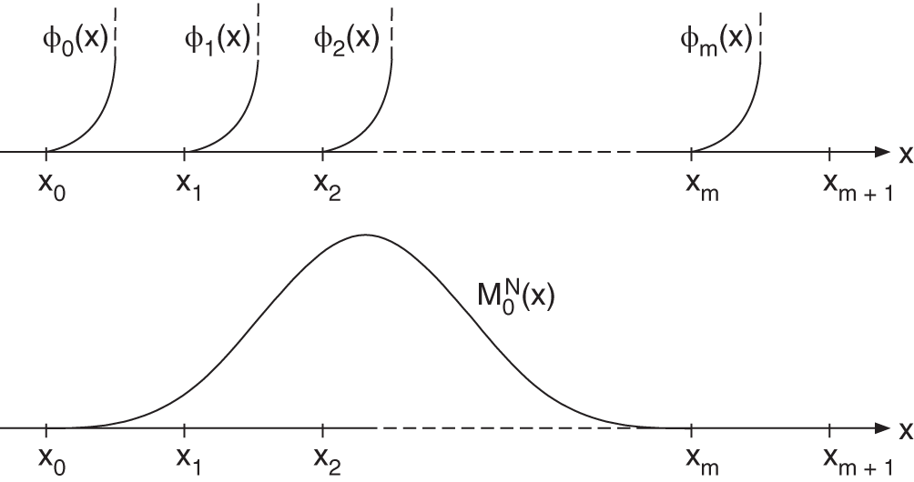
Figure 3.22 Truncated power functions and the B‐spline of Nth order.
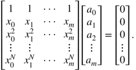
With the condition ![]() for
for ![]() , the following set of linear equations can be written with Eq. (3.80) and the coefficients of the powers of
, the following set of linear equations can be written with Eq. (3.80) and the coefficients of the powers of ![]() :
:
The homogeneous set of linear equations has nontrivial solutions for ![]() . The minimum requirement results in
. The minimum requirement results in ![]() . For
. For ![]() , the coefficients [Boe93] can be obtained as follows:
, the coefficients [Boe93] can be obtained as follows:
Setting the ![]() th column of the determinant in the numerator of Eq. (3.82) equal to zero corresponds to deleting the column. Computing both determinants of Vandermonde matrices [Bar90] and division leads to the coefficients
th column of the determinant in the numerator of Eq. (3.82) equal to zero corresponds to deleting the column. Computing both determinants of Vandermonde matrices [Bar90] and division leads to the coefficients

and hence

For some ![]() , we obtain
, we obtain

Because the functions ![]() decrease with increasing
decrease with increasing ![]() , a normalization of the form
, a normalization of the form ![]() is done, such that for equidistant samples, we get
is done, such that for equidistant samples, we get
The next example illustrates the computation of B‐splines.
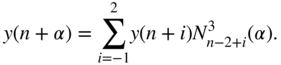
A linear combination of B‐splines is called a spline. Figure 3.24 shows the interpolation of sample ![]() for splines of second and third orders. The shifted B‐splines
for splines of second and third orders. The shifted B‐splines ![]() are evaluated at the vertical line representing the distance
are evaluated at the vertical line representing the distance ![]() . With sample
. With sample ![]() and the normalized B‐splines
and the normalized B‐splines ![]() , the second‐ and third‐order splines are expressed as
, the second‐ and third‐order splines are expressed as

The computation of a second‐order B‐spline at the sample index ![]() is based on the symmetry properties of the B‐spline, which is depicted in Fig. 3.25. With (Eqs. 3.77) and (3.86), and with the symmetry properties shown in Fig. 3.25, the B‐splines can be written in the form of
is based on the symmetry properties of the B‐spline, which is depicted in Fig. 3.25. With (Eqs. 3.77) and (3.86), and with the symmetry properties shown in Fig. 3.25, the B‐splines can be written in the form of
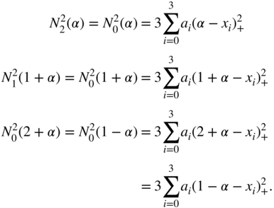

Figure 3.23 Third‐order B‐spline ( ,
,  , five samples).
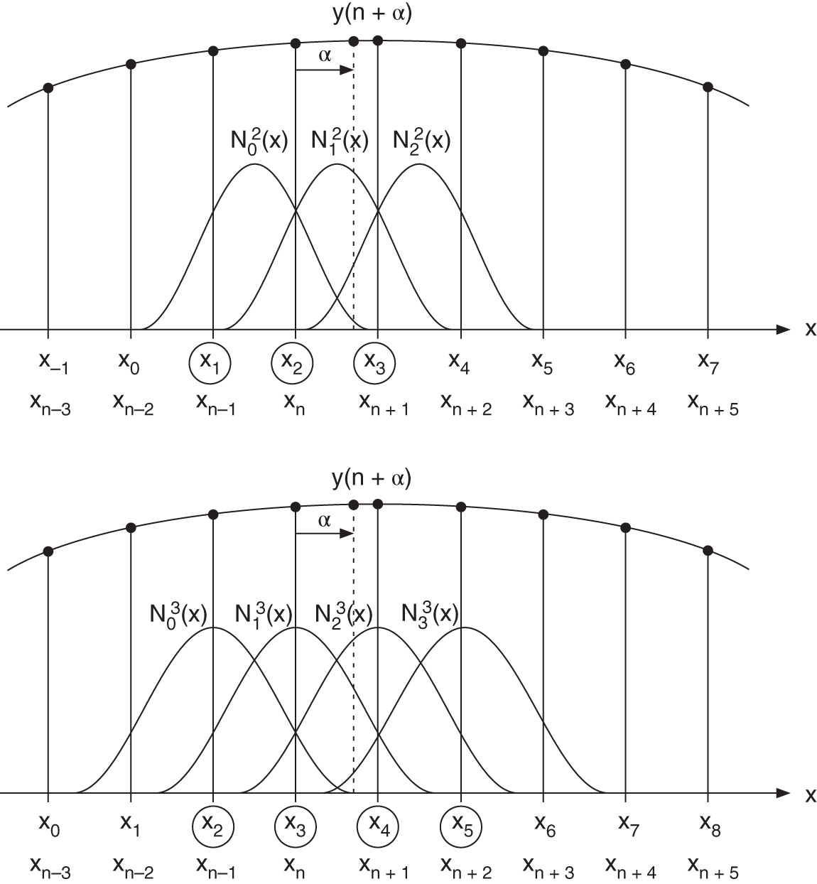
Figure 3.24 Interpolation with B‐splines of second and third orders.
With Eq. (3.83), we get the coefficients

and thus
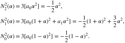
Owing to the symmetrical properties of the B‐splines, the time‐variant coefficients of the second‐order B‐spline can be derived as
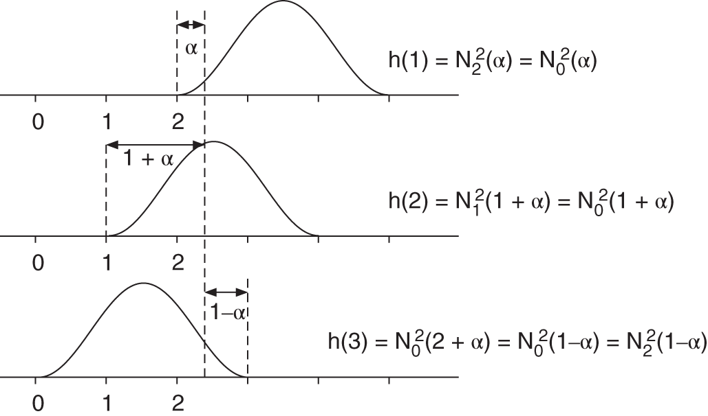
Figure 3.25 Exploiting the symmetry properties of a second‐order B‐spline.
In the same way, the time‐variant coefficients of a third‐order B‐spline are given by
Higher‐order B‐splines are given by
Similar sets of coefficients can be derived here as well. Figure 3.26 illustrates this for fourth‐ and sixth‐order B‐splines.
Generally, for even orders, we get
and for odd orders,


Figure 3.26 Interpolation with B‐splines of fourth and sixth order.
For the application of interpolation, the properties in the frequency domain are important. The zero‐order B‐spline is given by

and the Fourier transform gives the ![]() function in the frequency domain. The first‐order B‐spline, given by
function in the frequency domain. The first‐order B‐spline, given by

leads to a ![]() function in the frequency domain. Higher‐order B‐splines can be derived by repeated convolution [Chu92] as given by
function in the frequency domain. Higher‐order B‐splines can be derived by repeated convolution [Chu92] as given by
Thus, the Fourier transform leads to
With the help of the properties in the frequency domain, the necessary order of the spline interpolation can be determined. Owing to the attenuation properties of the ![]() function and the simple real‐time calculation of the coefficients, spline interpolation is well suited to time‐variant conversion in the last stage of a multistage sampling rate conversion system [Zöl94].
function and the simple real‐time calculation of the coefficients, spline interpolation is well suited to time‐variant conversion in the last stage of a multistage sampling rate conversion system [Zöl94].
3.5 Exercises
1. Basics
Consider a simple sampling rate conversion system with a conversion rate of ![]() . The system consists of two upsampling blocks, each by a factor of 2, and one downsampling block by a factor of 3.
. The system consists of two upsampling blocks, each by a factor of 2, and one downsampling block by a factor of 3.
- What are anti‐imaging and anti‐aliasing filters and where do we need them in our system?
- Sketch the block diagram.
- Sketch the input, intermediate, and output spectra in the frequency domain.
- How is the amplitude affected by the up‐ and downsampling and where does it come from?
- Sketch the frequency response of the anti‐aliasing and anti‐imaging filters needed for this upsampling system.
2. Synchronous Conversion
Our system will now be upsampled directly by a factor of 4 and again downsampled by the factor of 3, but with linear interpolation and decimation methods. The input signal is ![]()
![]() .
.
- What are the impulse responses of the two interpolation filters? Sketch their magnitude responses.
- Plot the signals (input, intermediate, and output signal) in the time domain using Matlab.
- What is the delay resulting from the causal interpolation/decimation filters?
- Show the error introduced by this interpolation/decimation method in the frequency domain.
3. Polyphase Representation
Now we extend our system using a polyphase decomposition of the interpolation/decimation filters.
- Sketch the idea of polyphase decomposition using a block diagram. What is the benefit of such decomposition?
- Calculate the polyphase filters for up‐ and downsampling (using interpolation and decimation).
- Plot with Matlab all resulting signals in the time and frequency domains.
4. Asynchronous Conversion
- What is the basic concept of asynchronous sampling rate conversion?
- Sketch the block diagram and discuss the individual operations.
- What is the necessary oversampling factor
 for a 20‐bit resolution?
 - How can we simplify the oversampling operations?
- How can we make use of polyphase filtering?
- Why are half‐band filters an efficient choice for the upsampling operation?
- Which parameters determine the interpolation algorithms in the last stage of the conversion?
References
- [Ada92] R. Adams, T. Kwan: VLSI Architectures for Asynchronous Sample‐Rate Conversion, Proc. 93rd AES Convention, San Francisco, Preprint No. 3355, October 1992.
- [Ada93] R. Adams, T. Kwan: Theory and VLSI Implementations for Asynchronous Sample‐Rate Conversion, Proc. 94th AES Convention, Berlin, Preprint No. 3570, March 1993.
- [Bar90] S. Barnett: Matrices ‐ Methods and Applications, Oxford University Press, 1990.
- [Boe93] W. Boehm, H. Prautzsch: Numerical Methods, AK Peters/Vieweg, 1993.
- [Chu92] C.K. Chui (ed.): Wavelets: A Tutorial in Theory and Applications, Volume 2, Academic Press, Boston, 1992.
- [Cro83] R.E. Crochiere, L.R. Rabiner: Multirate Digital Signal Processing, Prentice‐Hall, Englewood Cliffs, 1983.
- [Cuc91] S. Cucchi, F. Desinan, G. Parladori, G. Sicuranza: DSP Implementation of Arbitrary Sampling Frequency Conversion for High Quality Sound Application, Proc. IEEE ICASSP‐91, Toronto, pp. 3609–3612, May 1991.
- [Fli00] N. Fliege: Multirate Digital Signal Processing, J. Wiley & Sons, Chichester, 2000.
- [Hsi87] C.‐C. Hsiao: Polyphase Filter Matrix for Rational Sampling Rate Conversions, Proc. IEEE ICASSP‐87, Dallas, pp. 2173–2176, April 1987.
- [Kat85] Y. Katsumata, O. Hamada: A Digital Audio Sampling Frequency Converter Employing New Digital Signal Processors, Proc. 79th AES Convention, New York, Preprint No. 2272, October 1985.
- [Kat86] Y. Katsumata, O. Hamada: An Audio Sampling Frequency Conversion Using Digital Signal Processors, Proc. IEEE ICASSP‐86, Tokyo, pp. 33–36, 1986.
- [Lag81] R. Lagadec, H.O. Kunz: A Universal, Digital Sampling Frequency Converter for Digital Audio, Proc. IEEE ICASSP‐81, Atlanta, pp. 595–598, April 1981.
- [Lag82a] R. Lagadec, D. Pelloni, D. Weiss: A Two‐Channel Professional Digital Audio Sampling Frequency Converter, Proc. 71st AES Convention, Montreux, Preprint No. 1882, March 1982.
- [Lag82b] D. Lagadec, D. Pelloni, D. Weiss: A 2‐Channel, 16‐Bit Digital Sampling Frequency Converter for Professional Digital Audio, Proc. IEEE ICASSP‐82, Paris, pp. 93–96, May 1982.
- [Lag82c] R. Lagadec: Digital Sampling Frequency Conversion, Digital Audio, Collected Papers from the AES Premier Conference, pp. 90–96, June 1982.
- [Lag83] R. Lagadec, D. Pelloni, A. Koch: Single‐Stage Sampling Frequency Conversion, Proc. 74th AES Convention, New York, Preprint No. 2039, October 1983.
- [Liu92] G.‐S. Liu, C.‐H. Wei: A New Variable Fractional Delay Filter with Nonlinear Interpolation, IEEE Trans. Circuits and Systems‐II: Analog and Digital Signal Processing, Vol. 39, No.2, pp. 123–126, February 1992.
- [Opp99] A.V. Oppenheim, R.W. Schafer, J.R. Buck: Discret‐time Signal Processing, Prentice‐Hall, 2nd Edition, 1999.
- [Par90] S. Park, R. Robles: A Real‐Time Method for Sample‐Rate Conversion from CD to DAT, Proc. IEEE Int. Conf. Consumer Electronics, Chicago, pp. 360–361, June 1990.
- [Par91a] S. Park: Low Cost Sample Rate Converters, Proc. NAB Broadcast Engineering Conference, Las Vegas, April 1991.
- [Par91b] S. Park, R. Robles: A Novel Structure for Real‐Time Digital Sample‐Rate Converters with Finite Precision Error Analysis, Proc. IEEE ICASSP‐91, Toronto, pp. 3613–3616, May 1991.
- [Ram82] T.A. Ramstad: Sample‐Rate Conversion by Arbitrary Ratios, Proc. IEEE ICASSP‐82, Paris, pp. 101–104, May 1982.
- [Ram84] T.A. Ramstad: Digital Methods for Conversion Between Arbitrary Sampling Frequencies, IEEE Transactions on Acoustics, Speech and Signal Processing, vol. ASSP‐ 32, no. 3, pp. 577–591, June 1984.
- [Smi84] J.O. Smith, P. Gossett: A Flexible Sampling‐Rate Conversion Method, Proc. IEEE ICASSP‐84, pp. 19.4.1–19.4.4, 1984.
- [Sti91] E.F. Stikvoort: Digital Sampling Rate Converter with Interpolation in Continuous Time, Proc. 90th AES Convention, Paris, Preprint No. 3018, Feb. 1991.
- [Vai93] P.P. Vaidyanathan: Multirate Systems and Filter Banks, Prentice‐Hall, Englewood Cliffs, 1993.
- [Zöl94] U. Zölzer, T. Boltze: Interpolation Algorithms: Theory and Application, Proc. 97th AES Convention, San Francisco, Preprint No. 3898, November 1994.