CHAPTER 5
Stacks and Queues
Stacks and queues are relatively simple data structures that store objects in either first-in-first-out order or last-in-first-out order. They expand as needed to hold additional items, much like linked lists can, as described in Chapter 3, “Linked Lists.” In fact, you can use linked lists to implement stacks and queues.
You can also use stacks and queues to model analogous real-world scenarios, such as service lines at a bank or supermarket. Usually, however, they are used to store objects for later processing by other algorithms, such as shortest-path algorithms.
This chapter describes stacks and queues. It explains what they are, explains stack and queue terminology, and describes the methods that you can use to implement them.
Stacks
A stack is a data structure where items are added and removed in last-in-first-out order. Because of this last-in-first-out (LIFO, usually pronounced “life-oh”) behavior, stacks are sometimes called LIFO lists or LIFOs.
A stack is similar to a pile of books on a desk. You can add a book to the top of the pile or remove the top book from the pile, but you can't pull a book out of the middle or bottom of the pile without making the whole thing topple over.
A stack is also similar to a spring-loaded stack of plates at a cafeteria. If you add plates to the stack, the spring compresses so that the top plate is even with the countertop. If you remove a plate, the spring expands so that the plate that is now on top is still even with the countertop. Figure 5.1 shows this kind of stack.

Figure 5.1: A stack is similar to a stack of plates at a cafeteria.
Because this kind of stack pushes plates down into the counter, this data structure is also sometimes called a pushdown stack. Adding an object to a stack is called pushing the object onto the stack, and removing an object from the stack is called popping the object off of the stack. A stack class typically provides Push and Pop methods to add items to and remove items from the stack.
The following sections describe a few of the more common methods for implementing a stack.
Linked-List Stacks
Implementing a stack is easy using a linked list. The Push method simply adds a new cell to the top of the list, and the Pop method removes the top cell from the list.
The following pseudocode shows the algorithm for pushing an item onto a linked-list stack:
Push(Cell: sentinel, Data: new_value)// Make a cell to hold the new value.Cell: new_cell = New Cellnew_cell.Value = new_value// Add the new cell to the linked list.new_cell.Next = sentinel.Nextsentinel.Next = new_cellEnd Push
The following pseudocode shows the algorithm for popping an item off of a linked-list stack:
Data: Pop(Cell: sentinel)// Make sure there is an item to pop.If (sentinel.Next == null) Then <throw an exception>// Get the top cell's value.Data: result = sentinel.Next.Value// Remove the top cell from the linked list.sentinel.Next = sentinel.Next.Next// Return the result.Return resultEnd Pop
Figure 5.2 shows the process. The top image shows the stack after the program has pushed the letters A, P, P, L, and E onto it. The middle image shows the stack after the new letter S has been pushed onto the stack. The bottom image shows the stack after the S has been popped off of the stack.

Figure 5.2: It's easy to build a stack with a linked list.
With a linked list, pushing and popping items both have ![]() run times, so both operations are quite fast. The list requires no extra storage aside from the links between cells, so linked lists are also space-efficient.
run times, so both operations are quite fast. The list requires no extra storage aside from the links between cells, so linked lists are also space-efficient.
Array Stacks
Implementing a stack in an array is almost as easy as implementing one with a linked list. Allocate space for an array that is large enough to hold the number of items that you expect to put in the stack. Then use a variable to keep track of the next empty position in the stack.
The following pseudocode shows the algorithm for pushing an item onto an array-based stack:
Push(Data: stack_values [], Integer: next_index, Data: new_value)// Make sure there's room to add an item.If (next_index == <length of stack_values>) Then<throw an exception>// Add the new item.stack_values[next_index] = new_value// Increment next_index.next_index = next_index + 1End Push
The following pseudocode shows the algorithm for popping an item off of an array-based stack:
Data: Pop(Data: stack_values[], Integer: next_index)// Make sure there is an item to pop.If (next_index == 0) Then <throw an exception>// Decrement next_index.next_index = next_index - 1// Return the top value.Return stack_values[next_index]End Pop
Figure 5.3 shows the process graphically. The top image shows the stack after the program has pushed the letters A, P, P, L, and E onto it. The middle image shows the stack after the new letter S has been pushed onto the stack. The bottom image shows the stack after the S has been popped off of the stack.

Figure 5.3: It's easy to build a stack with an array.
With an array-based stack, adding and removing an item both have ![]() run times, so both operations are quite fast. Setting and getting a value from an array generally is faster than creating a new cell in a linked list, so this method may be slightly faster than using a linked list. The array-based stack also doesn't need extra memory to store links between cells.
run times, so both operations are quite fast. Setting and getting a value from an array generally is faster than creating a new cell in a linked list, so this method may be slightly faster than using a linked list. The array-based stack also doesn't need extra memory to store links between cells.
Unlike a linked-list stack, however, an array-based stack requires extra space to hold new items. How much extra space depends on your application and whether you know in advance how many items might need to fit in the stack. If you don't know how many items you might need to store in the array, you can resize the array if needed, although that will take extra time. If the array holds N items when you need to resize it, it will take ![]() steps to copy those items into the newly resized array.
steps to copy those items into the newly resized array.
Depending on how the stack is used, allowing room for extra items may be very inefficient. For example, suppose an algorithm occasionally needs to store 1,000 items in a stack, but most of the time it stores only a few. In that case, most of the time the array will take up much more space than necessary. If you know the stack will never need to hold more than a few items, however, an array-based stack can be fairly efficient.
Double Stacks
Suppose an algorithm needs to use two stacks whose combined size is bounded by some amount. In that case, you can store both stacks in a single array, with one at each end and both growing toward the middle, as shown in Figure 5.4.

Figure 5.4: Two stacks can share an array if their combined size is limited.
The following pseudocode shows the algorithms for pushing and popping items with two stacks contained in a single array. To make the algorithm simpler, the Values array and the NextIndex1 and NextIndex2 variables are stored outside of the Push methods.
Data: StackValues[<max items>]Integer: NextIndex1, NextIndex2// Initialize the array.Initialize()NextIndex1 = 0NextIndex2 = <length of StackValues> - 1End Initialize// Add an item to the top stack.Push1(Data: new_value)// Make sure there's room to add an item.If (NextIndex1 > NextIndex2) Then <throw an exception>// Add the new item.StackValues[NextIndex1] = new_value// Increment NextIndex1.NextIndex1 = NextIndex1 + 1End Push1// Add an item to the bottom stack.Push2(Data: new_value)// Make sure there's room to add an item.If (NextIndex1 > NextIndex2) Then <throw an exception>// Add the new item.StackValues[NextIndex2] = new_value// Decrement NextIndex2.NextIndex2 = NextIndex2 - 1End Push2// Remove an item from the top stack.Data: Pop1()// Make sure there is an item to pop.If (NextIndex1 == 0) Then <throw an exception>// Decrement NextIndex1.NextIndex1 = NextIndex1 - 1// Return the top value.Return StackValues[NextIndex1]End Pop1// Remove an item from the bottom stack.Data: Pop2()// Make sure there is an item to pop.If (NextIndex2 == <length of StackValues> - 1)Then <throw an exception>// Increment NextIndex2.NextIndex2 = NextIndex2 + 1// Return the top value.Return StackValues[NextIndex2]End Pop2
Stack Algorithms
Many algorithms use stacks. For example, some of the shortest path algorithms described in Chapter 13, “Basic Network Algorithms,” can use stacks. The following sections describe a few other algorithms that you can implement by using stacks.
Reversing an Array
Reversing an array is simple with a stack. Just push each item onto the stack and then pop it back off. Because of the stack's LIFO nature, the items come back out in reverse order.
The following pseudocode shows this algorithm:
ReverseArray(Data: values[])// Push the values from the array onto the stack.Stack: stack = New StackFor i = 0 To <length of values> - 1stack.Push(values[i])Next i// Pop the items off the stack into the array.For i = 0 To <length of values> - 1values[i] = stack.Pop()Next iEnd ReverseArray
If the array contains ![]() items, this algorithm takes
items, this algorithm takes ![]() steps, so it has run time
steps, so it has run time ![]() .
.
Train Sorting
Suppose a train contains cars bound for several different destinations, and it enters a train yard. Before the train leaves the yard, you need to use holding tracks to sort the cars so that the cars going to the same destination are grouped together.
Figure 5.5 shows a train with cars bound for cities 3, 2, 1, 3, and 2 entering from the left on the input track. The train can move onto a holding track and move its rightmost car onto the left end of any cars on that holding track. Later, the train can go back to the holding track and move a car from the holding track's left end back onto the train's right end. The goal is to sort the cars.

Figure 5.5: You can use stacks to model a train yard sorting a train's cars.
You can directly model this situation by using stacks. One stack represents the incoming train. Its Pop method removes a car from the right of the train, and its Push method moves a car back onto the right end of the train.
Other stacks represent the holding tracks and the output track. Their Push methods represent moving a car onto the left end of the track, and the Pop method represents moving a car off of the left end of the track.
The following pseudocode shows how a program could use stacks to model sorting the train shown in Figure 5.5. Here train is the train on the input track, track1 and track2 are the two holding tracks, and output is the output track on the right.
holding1.Push(train.Pop()) // Step 1: Car 2 to holding 1.holding2.Push(train.Pop()) // Step 2: Car 3 to holding 2.output.Push(train.Pop()) // Step 3: Car 1 to output.holding1.Push(train.Pop()) // Step 4: Car 2 to holding 1.train.Push(holding2.Pop()) // Step 5: Car 3 to train.train.Push(holding1.Pop()) // Step 6: Car 2 to train.train.Push(holding1.Pop()) // Step 7: Car 2 to train.train.Push(output.Pop()) // Step 8: Car 1 to train.
Figure 5.6 shows this process. The car being moved in each step has a bold outline. An arrow shows where each car moves.

Figure 5.6: You can sort this train in eight moves by using two holding tracks and an output track.
Tower of Hanoi
The Tower of Hanoi puzzle (also called the Tower of Brahma or Lucas' Tower), shown in Figure 5.7, has three pegs. One peg holds a stack of disks of different sizes, ordered from smallest to largest. The goal is to move all the disks from one peg to another. You must move disks one at a time, and you cannot place a disk on top of another disk that has a smaller radius.

Figure 5.7: The goal in the Tower of Hanoi puzzle is to restack disks from one peg to another without placing a disk on top of a smaller disk.
You can model this puzzle using three stacks in a fairly obvious way. Each stack represents a peg. You can use numbers giving the disks' radii for objects in the stacks.
The following pseudocode shows how a program could use stacks to model moving the disks from the left peg to the middle peg in Figure 5.7:
peg2.Push(peg1.Pop())peg3.Push(peg1.Pop())peg3.Push(peg2.Pop())peg2.Push(peg1.Pop())peg1.Push(peg3.Pop())peg2.Push(peg3.Pop())peg2.Push(peg1.Pop())
Figure 5.8 shows the process graphically.

Figure 5.8: You can model the Tower of Hanoi puzzle with three stacks.
One solution to the Tower of Hanoi puzzle is a nice example of recursion, so it is discussed in greater detail in Chapter 15, “Recursion.”
Stack Insertionsort
Chapter 6, “Sorting,” focuses on sorting algorithms, but Chapter 3 briefly explained how to implement insertionsort with linked lists. The basic idea behind insertionsort is to take an item from the input list and insert it into the proper position in a sorted output list (which initially starts empty). Chapter 3 explained how to implement insertionsort with linked lists, but you also can implement it with stacks.
The original stack holds items in two sections. The items farthest down in the stack are sorted, and those near the top of the stack are not. Initially, no items are sorted, and all of the items are in the “not sorted” section of the stack.
The algorithm uses a second, temporary stack. For each item in the original stack, the algorithm pops the top item off of the stack and stores it in a variable. It then moves all of the other unsorted items onto the temporary stack. By “moves,” I mean the algorithm pops a value from one stack and pushes it onto another stack.
Next the algorithm starts moving sorted items onto the temporary stack until it finds the position where the new item belongs within the sorted items. At that point, the algorithm inserts the new item onto the original stack and then moves all of the items from the temporary stack back onto the original stack. The algorithm repeats this process until all of the items have been added to the sorted section of the stack.
The following pseudocode shows the insertionsort algorithm at a fairly high level:
// Sort the items in the stack.StackInsertionsort(Stack: items)// Make a temporary stack.Stack: temp_stack = New StackInteger: num_items = <number of items>For i = 0 To num_items - 1// Position the next item.// Pull off the first item.Data: next_item = items.Pop()<Move the items that have not yet been sorted to temp_stack.At this point there are (num_items - i - 1) unsorted items.><Move sorted items to the second stack untilyou find out where next_item belongs.><Add next_item at this position.><Move the items back from temp_stack to the original stack.>Next iEnd StackInsertionsort
For each item, this algorithm moves the unsorted items to the temporary stack. Next it moves some of the sorted items to the temporary stack, and then it moves all of the items back to the original stack. At different steps, the number of unsorted items that must be moved is ![]() , so the total number of items moved is
, so the total number of items moved is ![]() . This means that the algorithm has a run time of
. This means that the algorithm has a run time of ![]() .
.
Stack Selectionsort
In addition to describing a linked-list insertionsort, Chapter 3 explained how to implement selectionsort with linked lists. The basic idea behind selectionsort is to search through the unsorted items to find the largest item and then move it to the front end of the sorted output list. Chapter 3 explained how to implement selectionsort with linked lists, but you can also implement it with stacks.
As in the insertionsort algorithm, the original stack holds items in two sections. The items farthest down in the stack are sorted, and those near the top of the stack are not. Initially, no items are sorted, and all of the items are in the “not sorted” section of the stack.
The algorithm uses a second temporary stack. For each position in the original stack, the algorithm moves all of the still unsorted items to the temporary stack, keeping track of the largest item.
After it has moved all of the unsorted items to the temporary stack, the program pushes the largest item it found onto the original stack in its correct position. It then moves all of the unsorted items from the temporary stack back to the original stack.
The algorithm repeats this process until all of the items have been added to the sorted section of the stack.
The following pseudocode shows the selectionsort algorithm at a fairly high level:
// Sort the items in the stack.StackSelectionsort(Stack: items)// Make the temporary stack.Stack: temp_stack = New StackInteger: num_items = <number of items>For i = 0 To num_items - 1// Position the next item.// Find the item that belongs in sorted position i.<Move the items that have not yet been sorted onto thetemp_stack, keeping track of the largest. Store thelargest item in variable largest_item.At this point there are (num_items - i - 1) unsorted items.><Add largest_item to the original stackat the end of the previously sorted items.><Move the unsorted items back from temp_stack to theoriginal stack, skipping largest_item when you find it>Next iEnd StackSelectionsort
For each item, this algorithm moves the unsorted items to the temporary stack, adds the largest item to the sorted section of the original stack, and then moves the remaining unsorted items back from the temporary stack to the original stack. For each position in the array, it must move the unsorted items twice. At different steps, there are ![]() unsorted items to move, so the total number of items moved is
unsorted items to move, so the total number of items moved is ![]() , and the algorithm has run time
, and the algorithm has run time ![]() .
.
Queues
A queue is a data structure where items are added and removed in first-in-first-out order. Because of this first-in-first-out (FIFO, usually pronounced “fife-oh”) behavior, stacks are sometimes called FIFO lists or FIFOs.
A queue is similar to a store's checkout queue. You join the end of the queue and wait your turn. When you get to the front of the queue, the cashier takes your money and gives you a receipt.
Usually, the method that adds an item to a queue is called Enqueue, and the item that removes an item from a queue is called Dequeue.
The following sections describe a few of the more common methods for implementing a queue.
Linked-List Queues
Implementing a queue is easy using a linked list. To make removing the last item from the queue easy, the queue should use a doubly linked list.
The Enqueue method simply adds a new cell to the top of the list, and the Dequeue method removes the bottom cell from the list.
The following pseudocode shows the algorithm for enqueueing an item in a linked-list stack:
Enqueue(Cell: top_sentinel, Data: new_value)// Make a cell to hold the new value.Cell: new_cell = New Cellnew_cell.Value = new_value// Add the new cell to the linked list.new_cell.Next = top_sentinel.Nexttop_sentinel.Next = new_cellnew_cell.Prev = top_sentinelEnd Enqueue
The following pseudocode shows the algorithm for dequeueing an item from a linked-list stack:
Data: Dequeue(Cell: bottom_sentinel)// Make sure there is an item to dequeue.If (bottom_sentinel.Prev == top_sentinel) Then <throw an exception>// Get the bottom cell's value.Data: result = bottom_sentinel.Prev.Value// Remove the bottom cell from the linked list.bottom_sentinel.Prev = bottom_sentinel.Prev.Prevbottom_sentinel.Prev.Next = bottom_sentinel// Return the result.Return resultEnd Dequeue
With a doubly linked list, enqueueing and dequeueing items have ![]() run times, so both operations are quite fast. The list requires no extra storage aside from the links between cells, so linked lists are also space-efficient.
run times, so both operations are quite fast. The list requires no extra storage aside from the links between cells, so linked lists are also space-efficient.
Array Queues
Implementing a queue in an array is a bit trickier than implementing one with a linked list. To keep track of the array positions that are in use, you can use two variables: Next, to mark the next open position, and Last, to mark the position that has been in use the longest. If you simply store items at one end of an array and remove them from the other, however, the occupied spaces move down through the array.
For example, suppose that a queue is implemented in an array with eight entries. Consider the following series of enqueue and dequeue operations:
Enqueue(M)Enqueue(O)Enqueue(V)Dequeue() // Remove M.Dequeue() // Remove O.Enqueue(I)Enqueue(N)Enqueue(G)Dequeue() // Remove V.Dequeue() // Remove I.
Figure 5.9 shows this sequence of operations. Initially, Next and Last refer to the same entry. This indicates that the queue is empty. After the series of Enqueue and Dequeue operations, only two empty spaces are available for adding new items. After that, it will be impossible to add new items to the queue.
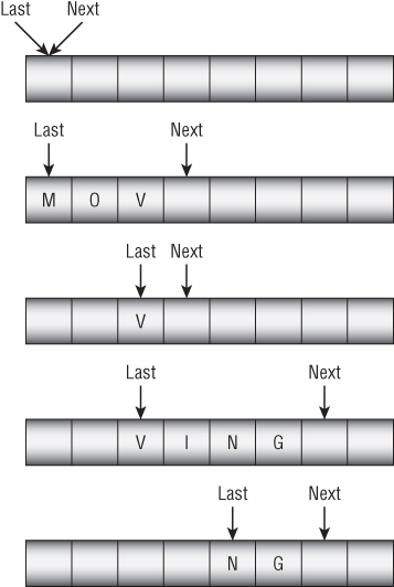
Figure 5.9: As you enqueue and dequeue items in an array-based queue, the occupied spaces move down through the array.
One approach to solving this problem is to enlarge the array when Next falls off the end of the array. Unfortunately, that would make the array grow bigger over time, and all the space before the Last entry would be unused.
Another approach would be to move all of the array's entries back to the beginning of the array whenever Last falls off the array. That would work, but it would be relatively slow.
A more effective approach is to build a circular array, in which you treat the last item as if it were immediately before the first item. Now when Next falls off the end of the array, it wraps around to the first position, and the program can store new items there.
Figure 5.10 shows a circular queue holding the values M, O, V, I, N, and G.

Figure 5.10: In a circular queue, you treat the array's last item as if it comes right before the first item.
A circular array does present a new challenge, however. When the queue is empty, Next is the same as Last. If you add enough items to the queue, Next goes all the way around the array and catches up to Last again, so there's no obvious way to tell whether the queue is empty or full.
You can handle this problem in a few ways. For example, you can keep track of the number of items in the queue, keep track of the number of unused spaces in the queue, or keep track of the number of items added to and removed from the queue. The CircularQueue sample program, which is available for download on the book's website, handles this problem by always keeping one of the array's spaces empty. If you added another value to the queue shown in Figure 5.10, the queue would be considered full when Next is just before Last, even though there was one empty array entry.
The following pseudocode shows the algorithm used by the example program for enqueueing an item:
// Variables to manage the queue.Data: Queue[<queue size>]Integer: Next = 0Integer: Last = 0// Enqueue an item.Enqueue(Data: value)// Make sure there's room to add an item.If ((Next + 1) Mod <queue size> == Last) Then <throw an exception>Queue[Next] = valueNext = (Next + 1) Mod <queue size>End Enqueue
The following pseudocode shows the algorithm for dequeueing an item:
// Dequeue an item.Data: Dequeue()// Make sure there's an item to remove.if (Next == Last) Then <throw an exception>Data: value = Queue[Last]Last = (Last + 1) Mod <queue size>Return valueEnd Dequeue
A circular queue still has a problem if it becomes completely full. If the queue is full and you need to add more items, then you need to allocate a larger storage array, copy the data into the new array, and then use the new array instead of the old one. This can take some time, so you should try to make the array big enough in the first place.
Specialized Queues
Queues are fairly specialized, but some applications use even more specialized queues. Two of these kinds of queues are priority queues and deques.
Priority Queues
In a priority queue, each item has a priority, and the dequeue method removes the item that has the highest priority. Basically, high-priority items are handled first.
One way to implement a priority queue is to keep the items in the queue sorted by priority. For example, you can use the main concept behind insertionsort to keep the items sorted. When you add a new item to the queue, you search through the queue until you find the position where it belongs and you place it there. To dequeue an item, you simply remove the top item from the queue. With this approach, enqueueing an item takes ![]() time, and dequeueing an item takes
time, and dequeueing an item takes ![]() time.
time.
Another approach is to store the items in whatever order they are added to the queue and then have the dequeue method search for the highest-priority item. With this approach, enqueueing an item takes ![]() time, and dequeueing an item takes
time, and dequeueing an item takes ![]() time.
time.
Both of these approaches are reasonably straightforward if you use linked lists.
The heap data structure described in the “Heapsort” section of Chapter 6 provides a more efficient way of implementing a priority queue. A heap-based priority queue can enqueue and dequeue items in ![]() time.
time.
Deques
Deque, which is usually pronounced “deck,” stands for double-ended queue. A deque is a queue that allows you to add items to and remove items from either end of the queue.
Deques are useful in algorithms where you have partial information about the priority of items. For example, you might know that some items are high priority and others are low priority, but you might not necessarily know the exact relative priorities of every item. In that case, you can add high-priority items to one end of the deque and low-priority items to the other end of the deque.
Deques are easy to build with doubly linked lists.
Binomial Heaps
You can use a linked list to make a simple priority queue, but then you need either to keep the list sorted (which is slow) or to dig through the list to find the highest-priority item when needed (which is also slow). A binomial heap lets you insert new items and remove the highest priority item relatively quickly.
A binomial heap contains a collection of binomial trees that contain the heap's values. To make rearranging the trees easier, the heap normally stores the tree roots in a linked list. You may want to use a list sentinel to make it easier to manage the list.
Chapters 10 and 11 have a lot more to say about trees, but I wanted to describe binomial heaps here near the discussion of priority queues.
Binomial Trees
You can define a binomial tree recursively by using the following rules:
- A binomial tree with order 0 is a single node.
- A binomial tree with order k has child nodes that are roots of subtrees that have orders
 in that order from left to right.
Figure 5.11 shows binomial trees with orders between 0 and 3. Dashed lines show how the order 3 contains trees of order 2, 1, and 0.

Figure 5.11: A binomial tree of order k contains binomial subtrees of order  .
.
Binomial trees have a couple of interesting properties. A tree of order ![]() contains
contains ![]() nodes and has a height of
nodes and has a height of ![]() . (A tree's height is the number of links between the root node and the tree's deepest leaf node.)
. (A tree's height is the number of links between the root node and the tree's deepest leaf node.)
A feature of binomial trees that is particularly important for building a binomial heap is that you can combine two trees of order ![]() by making one of the roots be a child of the other in order to produce a new tree of order
by making one of the roots be a child of the other in order to produce a new tree of order ![]() . Figure 5.12 shows how you can turn two order 2 trees into an order 3 tree.
. Figure 5.12 shows how you can turn two order 2 trees into an order 3 tree.

Figure 5.12: If you make the root of an order 2 tree (in the left dashed circle) into a child of the root of another order 2 tree (in the right dashed circle), you get an order 3 tree.
Binomial Heaps
A binomial heap contains a forest of binomial trees that follows these three additional rules:
- Each binomial tree obeys the minimum heap property. That means every node's value is less than or equal to the values of its children. In particular, this means that the tree's root holds the smallest value in the tree.
- The forest contains at most one binomial tree of any given order. For example, the forest might contain trees of order 0, 3, and 7, but it cannot contain a second tree with order 3.
- The forest's trees are sorted by their orders, so those with the smallest orders come first.
The first rule makes it easy to find the node with the smallest value in the forest—simply loop through the trees and pick the smallest root value.
The second property ensures that the heap cannot grow too wide and force you to examine a lot of trees when you need to find the smallest element.
In fact, the number of values in the heap uniquely determines the number of trees and their orders! Because a binomial tree of order ![]() contains
contains ![]() nodes, you can use the binary representation of the number of values to determine which trees it must contain.
nodes, you can use the binary representation of the number of values to determine which trees it must contain.
For example, suppose a heap contains 13 nodes. The binary representation of 13 is 1101, so the heap must contain a tree of order 3 (containing eight nodes), a tree of order 2 (containing four nodes), and a tree of order 0 (containing one node).
All of this means that a binomial heap containing ![]() nodes can hold at most
nodes can hold at most ![]() trees, so it cannot be too wide.
trees, so it cannot be too wide.
That's enough background about binomial trees and heaps. The following sections explain how you perform the key operations necessary to make a binomial heap work as a priority queue.
Merging Trees
As I mentioned earlier, you can merge two trees with the same order by making one tree's root a child of the other tree's root. The only trick here is that you need to maintain the minimum heap property. To do that, simply use the root node that has the smaller value as the parent so that it becomes the root of the new tree.
The following pseudocode shows the basic idea. Here I assume that the nodes in the trees are contained in BinomialNode objects. Each BinomialNode object has a NextSibling field that points to the node's sibling and a FirstChild field that points to the node's first child.
// Merge two trees that have the same order.BinomialNode: MergeTrees(BinomialNode: root1, BinomialNode: root2)If (root1.Value < root2.Value) Then// Make root1 the parent.root2.NextSibling = root1.FirstChildroot1.FirstChild = root2Return root1Else// Make root1 the parent.root1.NextSibling = root2.FirstChildroot2.FirstChild = root1Return root2End IfEnd MergeTrees
The algorithm compares the values of the trees' root nodes. If the value of root1 is smaller, the algorithm makes root2 a child of root1. To do that, it first sets the next sibling of root2 equal to the current first child of root1. It then sets the first child of root1 equal to root2, so root2 is the first child of root1 and its NextSibling pointer leads to the other children of root1. The algorithm then returns the new tree's root.
If the value of root2 is smaller than the value of root1, the algorithm performs the same steps with the roles of the two roots reversed.
Figure 5.13 shows this operation. The root nodes in the two trees on the left have values 24 and 16. Because 16 is smaller, that node becomes the root of the new tree and the node with value 24 becomes that node's child.

Figure 5.13: Merge two trees with the same order by making one tree's root become a child of the other tree's root.
Notice that the new tree satisfies the minimum heap property.
Merging Heaps
Merging two binomial heaps is the most important, interesting, and confusing operation required to maintain a binomial heap. The process works in two phases. First, you merge the tree lists. Then, you merge trees that have the same order.
Merging Tree Lists
In the first phase of merging two heaps, you merge the trees in each of the heaps into a single list where the trees are sorted in increasing order. Because each heap stores its trees in sorted order, you can loop through the two tree lists simultaneously and move the trees into the merged list in order.
The following pseudocode shows the basic idea. Here I assume that heaps are represented by BinomialHeap objects that have a RootSentinel property that points to the first tree in the heap's forest.
// Merge two heaps' tree lists.List Of BinomialTree: MergeHeapLists(BinomialHeap: heap1,BinomialHeap: heap2)// Make a list to hold the merged roots.BinomialNode: mergedListSentinel = New BinomialNode(int.MinValue)BinomialNode: mergedListBottom = mergedListSentinel// Remove the heaps' root list sentinels.heap1.RootSentinel = heap1.RootSentinel.NextSiblingheap2.RootSentinel = heap2.RootSentinel.NextSibling// Merge the two heaps' roots into one list in ascending order.While ((heap1.RootSentinel != null) And(heap2.RootSentinel != null))// See which root has the smaller order.BinomialHeap moveHeap = nullIf (heap1.RootSentinel.Order <= heap2.RootSentinel.Order) ThenmoveHeap = heap1ElsemoveHeap = heap2End If// Move the selected root.BinomialNode: moveRoot = moveHeap.RootSentinelmoveHeap.RootSentinel = moveRoot.NextSiblingmergedListBottom.NextSibling = moveRootmergedListBottom = moveRootmergedListBottom.NextSibling = nullEnd While// Add any remaining roots.If (heap1.RootSentinel != null) ThenmergedListBottom.NextSibling = heap1.RootSentinelheap1.RootSentinel = nullElse If (heap2.RootSentinel != null) ThenmergedListBottom.NextSibling = heap2.RootSentinelheap2.RootSentinel = nullEnd If// Return the merged list sentinel.Return mergedListSentinelEnd MergeHeapLists
This algorithm starts by setting each heap's RootSentinel value to the first actual tree in the heap. As long as both heaps contain trees, the code compares the first trees in the heaps (which will have the smallest orders in their respective heaps) and moves the one with the smaller order into the merged list.
After one of the heaps has run out of trees, the algorithm adds the other heap's remaining trees to the end of the merged list.
Figure 5.14 shows two heaps that should be merged.

Figure 5.14: The goal is to merge these two heaps.
Figure 5.15 shows the merged tree list.

Figure 5.15: This list contains the heaps' merged tree lists.
If you look at the merged tree list in Figure 5.15, you'll see that it violates second heap rule, which requires that a heap cannot contain more than one tree with the same order. This list contains two trees of order 1 and two trees of order 2. That brings us to the second phase of the merge process, merging trees that have the same order.
Merging Trees
In the second phase of merging two heaps, you merge any trees that have the same order. The trees in the merged list shown in Figure 5.15 are sorted by their orders. This means that if there are any trees with the same degree, then they are adjacent to each other in the list.
To merge the trees, you scan through the list looking for adjacent trees that have the same order. When you find a matching pair, you simply make one tree's root the child of the other tree's root as described earlier.
Unfortunately, there is a catch. When you merge two trees of order ![]() , you create a new tree of order
, you create a new tree of order ![]() . If the list happens to include two other trees of order
. If the list happens to include two other trees of order ![]() , then you now have three trees with the same order in a row. In that case, simply leave the first (new) tree alone and merge the following two trees into a new tree of degree
, then you now have three trees with the same order in a row. In that case, simply leave the first (new) tree alone and merge the following two trees into a new tree of degree ![]() .
.
The following pseudocode shows how to merge adjacent trees with the same order:
// Sift through the list and merge roots with the same order.MergeRootsWithSameOrder(BinomialNode: listSentinel)BinomialNode: prev = listSentinelBinomialNode: node = prev.NextSiblingBinomialNode: next = nullIf (node != null) Then next = node.NextSiblingWhile (next != null)// See if we need to merge node and next.If (node.Order != next.Order) Then// Move to consider the next pair.prev = nodenode = nextnext = next.NextSiblingElse// Remove them from the list.prev.NextSibling = next.NextSibling// Merge node and next.node = MergeTrees(node, next)// Insert the new root where the old ones were.next = prev.NextSiblingnode.NextSibling = nextprev.NextSibling = node// If we have three matches in a row,// skip the first one so we can merge// the other two in the next round.// Otherwise consider node and next// again in the next round.If ((next != null) And(node.Order == next.Order) And(next.NextSibling != null) And(node.Order == next.NextSibling.Order))Thenprev = nodenode = nextnext = next.NextSiblingEnd IfEnd IfEnd WhileEnd MergeRootsWithSameOrder
The algorithm uses three variables to keep track of its position in the merged tree list. The variable node points to the tree that the algorithm is considering. Variables prev and next point to the trees before and after node in the linked list.
The algorithm then enters a loop that executes as long as next is not null. If the node and next trees have different orders, the algorithm simply advances prev, node, and next to examine the next pair of trees.
If the node and next trees have the same order, then the algorithm calls the MergeTrees method described earlier to merge them. That may create a new tree with the same order as the next two trees. If that is the case, the algorithm advances prev, node, and next to move past the new tree so that it can merge the other two during the next pass through the While loop.
If the merge did not create three trees in a row with the same order, the algorithm leaves prev, node, and next so that node is pointing to the new tree. During the next trip through the loop, the algorithm will compare the new tree to the next one and merge them if they have the same order.
The next few figures show how the MergeRootsWithSameOrder algorithm works. Figure 5.16 shows the previous merged tree list, which contains some trees that have the same order.

Figure 5.16: Some of these trees have the same order, so they must be merged.
When the algorithm loops through the list, it finds that the trees inside the dashed ellipse shown in Figure 5.16 both have order 1, so it merges them into a tree with order 2. Figure 5.17 shows the new list.

Figure 5.17: The list now contains three trees in a row that have order 2.
When it merges the two trees with order 1, the algorithm notices that the list now contains three trees with order 2. It skips the first one and merges the second and third, which are surrounded by dashed lines in Figure 5.17.
Figure 5.18 shows the list after the latest merge.

Figure 5.18: At this point, the list ready to be used by a binomial heap.
Recall that the point of this exercise was to merge two binomial heaps. The MergeHeapLists algorithm merged their tree lists. Then the MergeRootsWithSameOrder algorithm merged any trees in the list that had the same order. At this point, the tree list satisfies the binomial heap properties, so you can use it to build the new merged heap. You'll see in the following sections how you can use this process to implement the final heap features: adding an item to the heap and removing the item with the smallest value from the heap.
Enqueue
After you know how to merge heaps, adding an item to a heap is relatively easy. Simply create a new heap that contains the new item and then merge the new heap with the existing one. The following pseudocode shows how to perform this operation:
Enqueue(Integer: value)// If this heap is empty, just add the value.If (RootSentinel.NextSibling == null) ThenRootSentinel.NextSibling = New BinomialNode(value)Else// Make a new heap containing the new value.BinomialHeap newHeap = New BinomialHeap()newHeap.Enqueue(value)// Merge with the new heap.MergeWithHeap(newHeap)End IfEnd Enqueue
This algorithm checks the heap's tree list to see whether it is empty. If the list is empty, it creates a new single-node (order 0) tree containing the new value and adds it to the top of the list.
If the tree list isn't empty, the algorithm makes a new single-item heap and then merges it with the existing heap.
Dequeue
After you know how to merge tree lists, removing the item with the smallest value is also easy. First, find the item with the smallest value and remove that item's tree from the tree list. Next, add the removed tree's child subtrees to a new heap and merge the new heap with the original one. The following pseudocode shows the steps in more detail:
// Remove the smallest value from the heap.Integer: Dequeue()// Find the root with the smallest value.BinomialNode: prev = FindRootBeforeSmallestValue()// Remove the tree containing the value from our list.BinomialNode: root = prev.NextSiblingprev.NextSibling = root.NextSibling// Make a new heap containing the// removed tree's subtrees.BinomialHeap: newHeap = New BinomialHeap()BinomialNode: subtree = root.FirstChildWhile (subtree != null)// Add this subtree to the top of the new heap's root list.BinomialNode: next = subtree.NextSiblingsubtree.NextSibling = newHeap.RootSentinel.NextSiblingnewHeap.RootSentinel.NextSibling = subtreesubtree = nextEnd While// Merge with the new heap.MergeWithHeap(newHeap)// Return the removed root's value.Return root.ValueEnd Dequeue
This algorithm finds the tree root that has the smallest value. Because each of the trees satisfies the minimum heap property, that is the item with the smallest value in the entire heap.
Next, the algorithm removes that tree from the tree list. It then creates a new heap and loops through the removed tree's subtrees adding them to the new heap. The subtrees of a binomial tree are stored sorted by increasing tree order, so it's easy to add them to the new heap in increasing order by simply adding them to the top of the new heap's tree list.
After it finishes adding the subtrees to the new heap, the algorithm calls the MergeWithHeap method to merge the new heap with the original one. The code finishes by returning the smallest item that it found.
Runtime
The longest operations on a binomial heap loop through the heap's tree list, so their runtimes depend on the length of that list. I mentioned earlier that the tree list can hold at most ![]() trees if the heap contains N items, so the time needed to loop through the list can take at most
trees if the heap contains N items, so the time needed to loop through the list can take at most ![]() time.
time.
More precisely, to enqueue an item, you create a new heap containing the item and then merge the new heap with the existing one. To merge the heaps, you combine their tree lists in ![]() time. You then loop through the merged tree list to combine any trees that have the same order, again taking
time. You then loop through the merged tree list to combine any trees that have the same order, again taking ![]() time. That makes the total time to insert an item
time. That makes the total time to insert an item ![]() .
.
To dequeue an item, you first spend ![]() time looping through the heap's tree list to find the root with the smallest value. You then remove that tree and add its subtrees to a new heap. The removed tree can have at most
time looping through the heap's tree list to find the root with the smallest value. You then remove that tree and add its subtrees to a new heap. The removed tree can have at most ![]() subtrees, so that takes at most
subtrees, so that takes at most ![]() time. Finally, you spend
time. Finally, you spend ![]() time merging the two heaps, so the total run time is
time merging the two heaps, so the total run time is ![]() .
.
The worst case time for inserting an item is ![]() , but in the long run the average time is smaller because a long operation tends to reduce the time needed for later operations.
, but in the long run the average time is smaller because a long operation tends to reduce the time needed for later operations.
For example, suppose a heap contains 15 items. Remember that the number of items uniquely determines the number and orders of the trees in the heap. If the heap contains 15 items, then it contains four trees with orders 0, 1, 2, and 3.
When you add another item, the new item will force all of those trees to merge together into a single tree of order 4 containing all 16 items. That operation will take the full ![]() steps because the heap initially contained
steps because the heap initially contained ![]() trees. However, after that, the heap contains only one tree, so future insertions will be much quicker.
trees. However, after that, the heap contains only one tree, so future insertions will be much quicker.
This kind of study of performance over a long sequence of operations is called amortized analysis. It turns out that the amortized runtime for inserting items in a binomial heap is ![]() .
.
Summary
This chapter explained stacks and queues, two data structures that are often used by other algorithms to store items. In a stack, items are added to and then removed from the same “end” of the data structure in last-in-first-out order. In a queue, items are added at one end and removed from the other in first-in-first-out order.
You can use an array to build a stack fairly easily, as long as it doesn't run out of space. If you build a stack with a linked list, you don't need to worry about running out of space.
You can also use an array to build a queue, although in that approach the items move through the array until they reach the end and you need to resize the array. You can solve that problem by using a circular array. You can also avoid the whole issue by using a doubly linked list to build a queue.
You can use stacks and queues to sort items in ![]() time, although those algorithms are more exercises in using stacks and queues than in efficient sorting. The next chapter describes several sorting algorithms that give much better performance, with some running in
time, although those algorithms are more exercises in using stacks and queues than in efficient sorting. The next chapter describes several sorting algorithms that give much better performance, with some running in ![]() time and others even running in
time and others even running in ![]() time.
time.
This chapter also explained binomial heaps, which are the most complicated data structures described by this book so far. They let you add and remove items from a heap in ![]() time. That makes them a useful method for building a priority queue.
time. That makes them a useful method for building a priority queue.
Exercises
You can find the answers to these exercises in Appendix B. Asterisks indicate particularly difficult problems.
- When you use a double stack, what is the relationship between the variables
NextIndex1andNextIndex2when one of the stacks is full? - Write an algorithm that takes as input a stack and returns a new stack containing the same items but in reverse order.
- Write a program that implements insertionsort with stacks.
- For each item, the stack insertionsort algorithm moves the unsorted items to the temporary stack. Next, it moves some of the sorted items to the temporary stack, and then it moves all of the items back to the original stack. Does it really need to move all of the items back to the original stack? Can you improve the algorithm's performance by modifying that step? What does that do to the algorithm's Big O run time?
- What does the stack insertionsort algorithm mean in terms of train sorting?
- Write a program that implements selectionsort with stacks.
- What does the stack selectionsort algorithm mean in terms of train sorting?
- Write a program that implements a priority queue.
- Write a program that implements a deque.
- *Consider a bank where customers enter a single line that is served by several tellers. You enter the line at the end, and when you get to the front of the line, you are served by the next available teller. You can model this “multiheaded queue” with a normal queue that serves multiple tellers.
Make a program similar to the one shown in Figure 5.19 to simulate a multiheaded queue in a bank. Give the user controls to adjust the number of tellers, the amount of time between customer arrivals, the amount of time each customer stays, and the speed of the simulation. After the user specifies the parameters, run a simulation to see how the queue behaves. How does the number of tellers affect the average wait time?

Figure 5.19: In a bank queue, customers stand in a single line and then are helped by the next available teller.
- Write a program that implements insertionsort with queues.
- Write a program that implements selectionsort with queues.
- *Write a program that implements a binomial heap.