9.1 The Finite ON–OFF Multirate Loss Model

9.1.2 The Analytical Model

9.1.2.1 Steady State Probabilities

To describe the analytical model in the steady state we present the following notations 1:

• : the vector of the number of in‐service service‐class k calls in state state ON, state OFF)
• ,
• 
• : a vector that shows a service‐class k call transition from state OFF to ON
• : a vector that shows a service‐class k call transition from state ON to OFF

the offered traffic‐load to state i from service‐class k; it is determined by:

(9.1)

where is the total arrival rate of service‐class k calls to state i and is given by:

(9.2)

is the external arrival rate of service‐class k calls to state i determined by:

(9.3)

is the and is given by (5.5a) and (5.5b).

Figure 9.1 shows the state transition rates of the f‐ON–OFF model (in equilibrium).

Assuming the existence of LB between adjacent states, the following LB equations are extracted from the state transition diagram of Figure 9.1:

(9.4a)

(9.4b)

(9.4c)

(9.4d)

where , , , , and are the probability distributions of the corresponding states , .

Equations (9.4b) and (9.4c) describe the balance between the rates of a new call arrival of service‐class k and the corresponding departure from the system, while (9.4a) and (9.4d) refer to the ON–OFF alternations of a service‐class k call. Based on the LB assumption, the probability distribution has a PFS which satisfies (9.4a)–(9.4d) and has the form [ 1]:

(9.5)

where is the normalization constant.

We now define by the b.u. held by a service‐class k call in state according to (5.10). We also define a matrix whose elements are the values of and let be the row of , where . In addition, let with where the occupied bandwidth of link real link, fictitious link) is given by (5.11).

Having found an expression for and since the CS policy is a coordinate convex policy (see Section I.12, Example I.30), the probability can be expressed by [ 1]:

(9.6)

where while , and .

Consider now the set of states whereby the occupied real and fictitious link bandwidths are exactly j and j , respectively. Then, the probability (links occupancy distribution) is denoted as in (5.13).

Summing (9.6) over we have:

(9.7)

The LHS of (9.7) is written as: . Since we continue by using the following change of variables:

Thus the LHS of ( 9.7) can be written as:

(9.8)

where , and . The first term of (9.8) is equal to , while the second term is written as:

where is the expected value of given .

By substituting the “new” first and second terms in ( 9.8), we have:

(9.9)

The RHS of ( 9.7) can be written as:

(9.10)

for and .

Combining (9.9) and (9.10), we have:

(9.11)

Multiplying both sides of (9.11) by and summing over , we have [ 1]:

(9.12)

The estimator in (9.12) is not known. To determine it, we use a lemma initially proposed in [2] for the determination of a similar estimator in the EnMLM. According to the lemma, two stochastic systems with (i) the same traffic description parameters and (ii) exactly the same set of states are equivalent, since they result in the same CBP. The purpose is therefore to find a new stochastic system in which we can determine the estimator . By choosing the bandwidth requirements of calls of all service‐classes and the capacities in the new stochastic system according to the criteria (i) conditions (a) and (b) are valid and (ii) each state has a unique occupancy , then each state can be reached only via state . Thus, the estimator and ( 9.12) can be written as (for ):

(9.13)

Equation (9.13) is the two‐dimensional recursive formula used for the determination of . The can be calculated in terms of an arbitrary under the normalization condition of . Although ( 9.13) is simple, it cannot be used for the determination of unless an equivalent system (mentioned above) is defined by enumeration and processing of the system's state space. The following example reveals the problems that can arise when one tries to use ( 9.13) prior to the state space enumeration and processing, and how these problems can be overcome.

Before we proceed with the determination of the various performance measures, we show the relationship between the f‐ON–OFF model and the EnMLM. These models are equivalent in the sense that they provide the same TC probabilities and CBP, when:

1. (i.e., when state OFF does not exist) for each service‐class . In that case the calculation of can be done via (6.27).
2. and . Then we can determine the mean holding time, , of a service‐class k call of the f‐ON–OFF model via (5.20). In that case, the f‐ON–OFF model is equivalent to the EnMLM with traffic parameters, and determined by (5.20).

9.1.2.2 TC Probabilities, CBP, and Utilization

The following performance measures can be determined based on ( 9.13):

• The TC probabilities of service‐class , via the formula [ 1]:
  (9.14)
  where .
• The CBP (or CC probabilities) of service‐class , via ( 9.14) but for a system with traffic sources.
• The link utilization, , via (5.19) where .

9.1.2.3 BBP

To illustrate the idea behind the formula for the BBP determination we consider Example 9.3.

Multiplying by the corresponding and the service rate in state OFF , we obtain the rate whereby service‐class  OFF calls would depart from the burst blocking state if it were possible. By summing these rates over the burst blocking state‐space we obtain the summation .

By normalizing it (taking into account the whole state space ), we obtain the following formula for the BBP calculation:

(9.15)

where and are calculated by ( 9.13).

Thus, (9.15) can be seen as the normalized rate of service‐class k OFF calls by which OFF calls would depart from the burst blocking states if it were possible.

For the record, the BBP of each service‐class in Example 9.3 are and , while the corresponding simulation results (with 95% confidence interval) are and .

9.2 Generalization of the f‐ON–OFF Model to include Service‐classes with a Mixture of a Finite and an Infinite Number of Sources

Consider a link with a pair of capacities and , accommodating service‐classes of finite ON–OFF sources (quasi‐random input) and service‐classes of infinite ON–OFF sources (random–Poisson input). Then, the calculation of the link occupancy distribution is done by the combination of ( 9.13) and (5.17) [3]:

(9.16)

Such a mixture of service‐classes does not destroy the accuracy of the model. The TC probabilities calculation can be done via ( 9.14), while the BBP calculation can be done via ( 9.15) for the service‐classes of finite population and via (5.39) for the service‐classes of infinite population.

9.3 Applications

An interesting application of the f‐ON–OFF model has been proposed in [4], where the OCDMA PON architecture of Figure 9.5 with ONUs is considered.

All ONUs are connected to the OLT through a passive optical splitter/combiner (PO‐SC). The PO‐SC is responsible for collecting data from all ONUs and transmitting them to the OLT (upstream direction), as well as for broadcasting data from the OLT to the ONUs (downstream direction). The analysis of [ 4] concentrates on the upstream direction; however, it can also be applied to the downstream direction. Users that are connected to an ONU alternate between active and passive (silent) transmission periods. The PON uses codewords, which have the same length and the same weight , while the auto‐correlation and cross‐correlation parameters are defined according to the desired BER at the receiver. The PON supports service‐classes which are differentiated via the parallel mapping technique. Under this technique, the OLT assigns codewords to a service‐class call for the entire duration of the call. More precisely, during the holding time of a service‐class call the data bits of this call are grouped per bits and transmitted in parallel in each bit period. One codeword is used to encode bit “1”, while data bit “0” is not encoded. Thus, the call uses a number of these codewords in each bit period and this number is equal to the number of data bits “1” that are transmitted during a bit period. In this way, the complex procedure of assigning codewords in each data bit period is avoided. Furthermore, since bits are transmitted in each data bit period, the data rate of service‐class is , where is the basic data rate of a single codeworded call.

When a single codeword is assigned to an active user (active call), the received power of this call at the OLT is denoted by ( corresponds to the received power per bit, for a specific value of the BER [5]). Since the PON supports multiple service‐classes of different data rates, a number of single codewords is assigned to each service‐class, therefore the received power of an active call of service‐class is proportional to , since data bits are simultaneously transmitted for service‐class during a bit period, therefore:

(9.17)

The connection establishment between the end‐user and the OLT is based on a three‐way handshake (request/ACK/confirmation). Calls of service‐class arrive at ONU from a finite number of traffic sources ; the total number of service‐class traffic sources in the PON is . The mean call arrival rate of service‐class is , where is the arrival rate per idle source, while and are the numbers of service‐class calls in the PON in the active and passive states, respectively. Calls that are accepted for service start an active period and may remain in the active state for their entire duration, or alternate between active and passive periods. During an active period, a burst of data is sent to the OLT, while no data transmission occurs throughout a passive period. When a service‐class call is transferred from the active to the passive state the total number of in‐service codewords is reduced by . When a passive call attempts to become active, it re‐requests the same number of codewords (but not necessarily the same codewords) as in the previous active state. If the total number of codewords in use does not exceed a maximum threshold (the PON capacity), the call begins a new active period, otherwise burst blocking occurs and the call remains in the passive state for another period. At the end of an active period, the call is transferred to the passive state with probability or departs from the system (the connection is terminated) with probability . The active and passive periods of service‐class calls are exponentially distributed with mean  ( indicates active state, indicates passive state).

In OCDMA systems, an arriving call should be blocked, after the new call acceptance, if the noise of all in‐service calls is increased above a predefined threshold; this noise is called multiple access interference (MAI). We differentiate the MAI from other forms of noise (thermal, fiber‐link, beat, and shot noise). The thermal noise and fiber link noise are typically modeled as Gauss distributions and , respectively, while the shot noise is modeled as a Poisson process [6]. The beat noise is modeled as a Gauss distribution [7]. According to the central limit theorem, we can assume that the total additive noise is modeled as a Gauss distribution , considering that the number of noise sources in the PON is relatively large. Therefore, the total interference caused by the thermal, the fiber‐link, the beat, and the shot noise is modeled as a Gauss distribution with mean and variance .

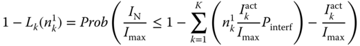
Upon a call arrival at an ONU, a CAC located at the OLT decides on its acceptance or rejection according to the total received power at the OLT. More precisely, the CAC estimates the total received power (together with the power of the new call); if it exceeds a maximum threshold , the call is blocked and lost. The maximum received power is calculated based on the worst case scenario that all data bits transmitted in parallel are “1”, in order to ensure that the BER will never increase above the desired value. The value of is also determined by the desired BER at the receiver [ 5]. This condition is expressed by the following relation:

(9.18)

The summation in (9.18) refers to the received power of all in‐service active calls of all service‐classes multiplied by the average probability of interference . This probability is a function of the weight , the length , and the maximum cross‐correlation parameter of the codewords, as well as of the hit probabilities between two codewords of different users. Specifically, the hit probabilities of getting hits during a bit period out of the maximum cross‐correlation value are given by [8]:

(9.19)

where the factor is due to the fact that data bit “0” is not encoded. In the case of , the percentage of the total power of a data bit that interferes with a bit of the new call is , since 1 out of “1” of the codewords may interfere. In this case . When , the probability of interference is given by:

(9.20)

The condition expressed by ( 9.18) is also examined at the receiver, when a passive call tries to become active. Based on ( 9.18), we define the LBP that a service‐class call is blocked due to the presence of the additive noise, when the number of in‐service active calls is , as:

(9.21)

or

(9.22)

Assuming that the total additive noise follows a Gauss distribution , the variable follows a Gauss distribution too. Therefore, the RHS of (9.22) is the CDF of the Gauss variable and is denoted as :

(9.23)

where is the well‐known error function.

By using ( 9.22) and (9.23), we can calculate of service‐class calls by substituting :

(9.24)

Now, let be the capacity of the (real) shared link, which is the PON capacity. This is discrete because it is expressed by the total number of codewords, which could be assigned to the PON users. When a call is transferred to a passive state, it is assumed that a number of fictitious codewords are assigned to it from a total number of fictitious codewords . That is, each passive call is accommodated in a fictitious shared link of fictitious discrete capacity [9]. The number of codewords assigned to a passive call is equal to the number of codewords assigned to the call at the active state.

To show the role of the fictitious system in call admission, let be the number of codewords of all active calls and be the number of codewords of all passive calls:

(9.25)

If an arriving call is not blocked because of local blocking, then the CAC works as follows, taking into account the hard blocking conditions of (5.1) and (5.2). Let be the set of all permissible states of the whole system (real and fictitious links), then the occupancy distribution of , denoted by , is given by a two‐dimensional approximate recursive formula, which is similar to ( 9.13):

(9.26)

where and for the real and the fictitious link, respectively, and is the occupied capacity of the system, given by:

(9.27)

and

(9.28)

9.4 Further Reading

Due to the relationship between the f‐ON–OFF model and the EnMLM (see Section 9.1.2.1), the f‐ON–OFF model can be extended to include various characteristics of the EnMLM extensions (see, e.g., Chapter ). Thus, the interested reader may actually study extensions of the EnMLM and consider as a candidate model the f‐ON–OFF model, especially when the combination of call blocking and burst blocking is necessary.

References

1. 1 I. Moscholios, M. Logothetis and M. Koukias, An ON–OFF multirate loss model of finite sources. IEICE Transactions on Communications, E90‐B(7):1608–1619, July 2007.
2. 2 G. Stamatelos and J. Hayes, Admission control techniques with application to broadband networks. Computer Communications, 17(9):663–673, September 1994.
3. 3 I. Moscholios, M. Logothetis and M. Koukias, An ON–OFF multi‐rate loss model with a mixture of service‐classes of finite and infinite number of sources. Proceedings of IEEE ICC, Seoul, Korea, May 2005.
4. 4 J. Vardakas, I. Moscholios, M. Logothetis and V. Stylianakis, Performance analysis of OCDMA PONs supporting multi‐rate bursty traffic. IEEE Transactions on Communications, 61(8):3374–3384, August 2013.
5. 5 C.‐S. Weng and J. Wu, Optical orthogonal codes with nonideal cross correlation. IEEE/OSA Journal of Lightwave Technology, 19(12):1856–1863, December 2001.
6. 6 W. Ma, C. Zuo and J. Lin, Performance analysis on phase‐encoded OCDMA communication system. IEEE/OSA Journal of Lightwave Technology, 20(5):798–803, May 2002.
7. 7 X. Wang and K. Kitayama, Analysis of beat noise in coherent and incoherent time‐spreading OCDMA. IEEE/OSA Journal of Lightwave Technology, 22(19):2226–2235, October 2004.
8. 8 H.‐W. Chen, G.‐C. Yang, C.‐Y. Chang, T.‐C. Lin and W. C. Kwong, Spectral efficiency study of two multirate schemes for asynchronous optical CDMA. IEEE/OSA Journal of Lightwave Technology, 27(14):2771–2778, July 2009.
9. 9 J. Vardakas, I. Moscholios, M. Logothetis and V. Stylianakis, On code reservation in multi‐rate OCDMA passive optical networks. Proceedings of IEEE CSNDSP, Poznan, Poland, July 2012.