
Chapter 13
Sustainment Related Models and Trade Studies
John E. MacCarthy
Systems Engineering Education Program, Institute for Systems Research, University of Maryland, College Park, MD, USA
Andres Vargas
Department of Industrial Engineering, University of Arkansas, Fayetteville, AR, USA
The sustainment key performance parameter (KPP) (Availability) is as critical to a program's success as cost, schedule, and performance.
(DoDI 5000.02 (2015))
13.1 Introduction
This chapter develops a number of “first-order” sustainment-related models1 for a relatively simple fictional remotely piloted air vehicle (i.e., drone) system that illustrates modeling techniques that are currently used to support reliability, availability, and maintainability (RAM) analysis, total life cycle cost analyses, and cost–RAM performance trade-off analyses. While the models developed in this chapter are based on simplifying assumptions and fictional data, they can provide a modeling framework for more complex RAM and life cycle cost analysis of real systems that use real data and fewer simplifying assumptions.
Sustainment trade studies are important from two perspectives – life cycle cost and system performance. Generally, 50% (or more) of a typical system's life cycle cost is associated with operations and maintenance (INCOSE, 2015). A large portion of these costs are typically associated with maintenance (which depends on system reliability). In addition, system availability (which depends on reliability and maintainability) is a system performance metric of particular importance to the operator.
Given the clear importance of system reliability, maintainability, and availability, the DoD has established a “Sustainment Key Performance Parameter (KPP)” that requires programs to include technical performance requirements for reliability and availability and cost estimates for maintenance (CJCSI 3170.01I, 2012). In addition, the Department of Defense Office of Acquisition, Technology, and Logistics (AT&L) has established guidance on sustainment that emphasizes the importance of including quantitative requirements for system reliability, maintainability, and availability (DoDI 5000.02, 2015).
For the purposes of this chapter, reliability is defined as the probability that a system or product [element/item/service] “will perform in a satisfactory manner for a given period of time, when used under specified operating conditions.” (Blanchard and Fabrycky, 2010). The principal metric used to specify a system's reliability is the mean time between failures (MTBF). Maintainability may be defined in two ways depending on whether one is most interested in the time required to repair the system or the cost of repairing the system. In the first case, maintainability is defined as “the probability that an item will be retained in or restored to a specified condition within a given period of time, when maintenance is performed in accordance with prescribed procedures and resources.” (Blanchard and Fabrycky, 2010). One common metric used to describe a system's maintainability is the mean downtime (MDT). In the second case, maintainability is defined as “the probability that the maintenance cost for the system will not exceed y dollars per designated period, when the system is operated in accordance with prescribed procedures.” (Blanchard and Fabrycky, 2010). One may use the system's mean life cycle maintenance cost as a metric for this aspect of maintainability. Finally, a system's operational availability is defined as “the probability that a system or equipment, when used under stated conditions in an actual operational environment, will operate satisfactorily when called upon.” (Blanchard and Fabrycky, 2010). The relationship between a system's availability, reliability, and maintainability is discussed in Section 13.2.1.1.
This chapter develops the RAM and life cycle cost models and demonstrates how a number of analytical techniques may be applied to find the most cost-effective design and to determine the performance uncertainty associated with different design solutions. Section 13.2 provides an example of how to build a model to calculate the reliability and availability of an unmanned air vehicle (UAV) system based on the system's logical system architecture. It also shows how such a model may be used to perform trade-off analyses between different system architectures (and reliability allocations to different elements), different operational concepts, different maintainability requirements, and different resulting system availabilities. Section 13.3 provides an example of how to build a model for the system's sustainment costs and how to use this model in tandem with the previously developed availability model to perform cost–performance (total life cycle cost vs Ao) trade-off analyses. Section 13.4 uses the modeling framework developed in Section 13.3 to develop an Excel model that employs an evolutionary optimization technique to find the lowest cost design solution that meets the system's availability requirement. The Excel model is also used to provide a “cost-effectiveness” tradespace curve and to perform a deterministic parameter sensitivity study to guide the development of the Monte Carlo (MC) model developed in Section 13.5. Finally, Section 13.5 provides an example of how to develop a Monte Carlo extension to the availability model developed in Section 13.2 and how such a model can be used to determine the confidence that one may have that a given design will be able to meet its availability requirement.
13.2 Availability Modeling and Trade Studies
This section develops an analytic model for the operational availability of a simple Forest Monitoring Drone System (FMDS) as a function of a variety of system and system element parameters. It then demonstrates how the model may be used to perform availability trade studies to identify architecture modifications that will enable the system to achieve a required system availability. The section also demonstrates how such a model may be used to perform sensitivity analyses. We begin by describing the FMDS mission, system architecture, operational concept, and maintenance concept. We then develop a state model for each element and use the existing body of research on how to model complex, standby systems. The result is a reliability block diagram (RBD) model that may be used to calculate the system-level mean time between critical failures (MTBCFs) and to develop the associated availability model.
13.2.1 FMDS Background
This section provides a quick overview of the system's mission, availability requirement, conceptual design/physical architecture, and concept of operation.
In our illustrative example, the USDA Forest Service is considering using drones to monitor a forest for fires. They want to be able to provide 24/7 coverage of the forest. The drone will generally fly an established repeated flight path (“orbit”) over the forest. It will be launched from an air field (base) that is about a 10 min flight from the forest. This geometry is outlined in Figures 13.1 and 13.2.

Figure 13.1 System operational concept

Figure 13.2 System operational concept (cont.)
We further suppose that the Forest Service has specified that the system must provide “an operational availability of coverage” of 80% (i.e., there must be a drone on orbit, under control and successfully reporting sensor data, 80% of the time).
The “System of Interest” (or system) consists of the mission elements, the maintenance element, and the personnel required to operate and maintain the mission elements. The mission elements consist of a number of drone/air vehicle elements (Nd) and a number of “control elements” (Nc), where Nd and Nc are to be determined through this analysis.
The drone will be launched from the air field and travel to its orbit. The drone carries enough fuel for up to 4 h of flight (maximum flight time Tmf). The drone is controlled by the “control element” that is located at the air field. The control element exercises control of the drone via a dedicated communications link supported by communications components of the drone and control elements. The control element also receives and displays the continuous, real-time sensor data provided by the drone via a dedicated communications downlink that is supported by communications components of the drone and control elements.
The typical mission timeline for a drone consists of preparing it for flight, launching it, flying it to station, monitoring the area (time on station), returning to base, landing, and postflight maintenance. Table 13.1 provides a summary of the nominal times associated with each mission activity. The “Time on Station Margin” reflects an expectation that one will generally want to return the drone to the airbase with some fuel to spare.
Table 13.1 Mission Activities and Nominal Times
| Activity/Time | Symbol | Nominal Time (h) |
| Maximum flight time | Tmf | 4.0 |
| Preflight preparation time | Tpfp | 0.5 |
| Time to launch | Tlch | 0.1 |
| Time to station | Tts | 0.2 |
| Time to return to base | Trtb | 0.2 |
| Time to land | Tlnd | 0.1 |
| Time on station margin | Tm | 0.3 |
| Time on station | Tos | Tmf–(Tlch+Tts+Trtb+Tlnd+Tm) = 3.1 |
| Postflight maintenance time (drone) | Tpfm | 1.0 |
We can see from the aforementioned timeline that the Time on Station (3.1 h) will be less than the maximum flight time (4 h). It should also be noted that there will be uncertainties associated with each of the nominal times indicated earlier.
In order for the Forest Service to maintain 24/7 monitoring of the forest, a second drone will need to be prepared for flight, launched, and reach its orbit to the first drone having to begin its return to base. Figure 13.3 provides and illustration of this timeline (not to scale). While each drone requires a dedicated control element to control its flight, any control element may be used with any drone.

Figure 13.3 Mission timeline
The drone is expected to have a mean time between critical failures (MTBCFd) of 50 h. The mean time between critical failures for the control element (MTBCFc) is expected to be 75 h. For the purposes of this chapter, a critical failure is a failure that results in an element being unable to perform its intended purpose, could lead to loss of the element, or injury to person or property. An element that experiences a critical failure may not be used until the failure is corrected.2 If a drone element experiences a (critical) failure, it must return to base and undergo unscheduled (corrective) maintenance. The downtime associated with unscheduled maintenance (Tdum) will be discussed in more detail in the following section. If a second drone is not already in the process of preparing for flight, launching, or flying to station, it must begin preparation for flight and take the place of the failed drone as quickly as possible (see timeline). A drone that is undergoing maintenance (scheduled or unscheduled) may not begin flight preparation until its maintenance is completed.
If a control element experiences a failure and a second control element is available, it may be used. The downtime associated with “swapping in” the backup control element (Tcs) is nominally expected to be 0.1 h. The failed control element will then undergo unscheduled maintenance. The unscheduled maintenance downtime associated will be addressed in the following section.
13.2.1.1 The FMDS Analytic Availability Model
This subsection develops the analytic availability model for the FMDS that will be used to perform a series of availability trade studies. A system's (steady-state) operational availability is defined as its uptime divided by the sum of its uptime and downtime. Given this definition, and ignoring the effects of scheduled maintenance, if MTBCFS is the system's MTBCF and MDTs is the MDT associated with a critical system failure, it follows that:
Now consider a system that has some number of independent failure modes (Nf), each characterized by a constant failure rate λi and MDTi.3 The system failure rate will be λs = ∑λi and the mean system downtime (MDTs) will be a frequency-weighted average of the individual wait times, MDTs = ∑(MDTi*λi/λs). Using the fact that MTBCFS = 1/λs we have:

The ∑(MDTi/MTBCFi) may be thought of a normalized “failure rate-weighted downtime.”
Section 13.2.1.2 develops the reliability models required to identify the failure modes and to calculate the MTBCF for each identified failure mode. Section 13.2.1.3 provides a maintenance concept for the system and develops expressions for the MDT associated with each failure mode. Furthermore, Section 13.2.1.4 provides an influence diagram for the FMDS System. Finally, Section 13.2.1.5 discusses an integrated Excel implementation of equation 13.2, and the MTBFi and MDTi expressions are developed Sections 13.2.1.2 and 13.2.1.3.
13.2.1.2 Reliability Models and Failure Modes
This section develops an RBD for our system (the FMDS), which is then used to identify the principal system-level failure modes. We will see that the FMDS is a relatively simple example of what is termed a “complex structure”.4 Some of the techniques developed in the current literature on complex structures5 will be used to develop expressions that will permit us to calculate values for system-level MTBFs, based on the element-level MTBFs and associated downtimes.
Figure 13.4. provides the RBD for our system of interest. We see that the FMDS consists of two “substructures” (a control substructure and a drone substructure) that operate in series. Each substructure is in turn composed of two or more elements organized in a parallel manner. The “disconnections” in the structures indicate that the “standby elements” do not “kick in” until the active element fails and that there is a “downtime” associated with the switch. Such elements are referred to as “cold standby” elements. The control and drone “substructures” are examples of “1-out-of-N cold standby” structures.6
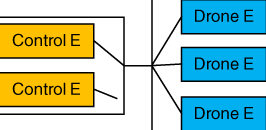
Figure 13.4 System reliability block diagram
We define a “system failure” to be an event that results in a potential interruption to time on station. There are two types of system failures: (i) an element failure where a standby element is available (Type 1 failure) and (ii) an element failure where a standby element is unavailable7 (Type 2 failure). Generally, the mean system downtime associated with a Type 1 failure will be much shorter than the MDT associated with a Type 2 failure.
An “element failure” is defined to be an event that requires one element to be replaced by an identical backup element. Given this definition, for simplicity, we will assume that the only event that would lead a control element to have to be replaced by a backup would be a control element critical failure. In the case of Type 1 control element critical failures, the mean time between critical control element failures will be denoted by “MTBCF1c” (which was earlier assumed to have a nominal value of 75 h). The mean system downtime associated with this kind of failure will be denoted “MDT1c.” This is just the time it takes to power up the backup control element (hardware and software) and to establish the required communications links. We assume a nominal value of 0.1 h. In the case of Type 2 control element failures, the mean time between Type 2 control element failures will be denoted by “MTBCF2c” and the associated downtime is denoted by “MDT2c.” The value of MDT2c depends on the maintenance concept and is a topic of discussion in the next subsection. Birolini (2007) (and Kuo & Zuo, 2003) developed a recursion formula that may be used to calculate the MTBCF2c. A “structure” (or substructure) consisting of n parallel elements in which k of the elements must be operating for the system to operate and the remaining n − k elements are not operating (cold), but serve as “standbys” in the case of a failure of one of the operating units is referred to as a “k-out-of-n cold standby” structure. When an element fails, it goes into repair. The number of failed elements than may go be simultaneously repaired is limited by the number of “repair crews.” In our analysis, we will consider the case of “1-out-of-n cold standby” substructures where there is only one repair crew. In this case, the recursion formula takes the simpler form:

where the subscript “e” indicates either a control or drone element, μe = 1/MDTe, λe = 1/MTBCFe, and MTBCFS(0) is the MTBCF for the substructure.
Applying this recursion formula to the case of a substructure consisting of one active unit and one standby unit (a “1-out-of-2 cold standby” structure), with a single repair crew8, the control substructure's MTBF may be shown to be:
The case of the drone is a bit more complicated. Here we assume that there are two events that could lead to a Drone Element having to be replaced. First, a drone runs low on fuel and must return to base (a scheduled return to base “failure”). We denote the mean time between scheduled returns to base (SRTB) events by “MTBSRTB1d,”which may be determined using:
Second, a drone may experience a critical failure and have to return to base earlier than planned. This is just the MTBCFS for the drone, denoted as “MTBCF1d” (which was earlier assumed to have a nominal value of 50 h).
Each of these failure modes results in a different mean system downtimes. We denote the mean system downtime associated with a SRTB by “MDT1srtb.” If a standby drone is prepared and launched in time to reach orbit prior to the on-station drone having to return (which is assumed to be the case), there is no associated system downtime (i.e., MDT1srtb = 0). We denote the mean system downtime associated with a critical failure is denoted by “MDT1d.” Since this is unexpected, the system is down until an available standby drone may be prepared, launched and transit to station. As such, a nominal value for MDT1d may be calculated using:
In the case of Type 2 drone element failures, if one assumes that the mean system downtime associated with bringing a replacement drone that is currently in maintenance back to active on-station status (denoted by “MDT2d”) is the same regardless of whether the returning drone is returning due to a SRTB or a critical failure, one may define an “effective” MTBCFS for the drone MTBCF1de, that includes both critical failures and SRTBs, as

and use the recursion formula for a “1-out-of-3 cold standby” structure (assuming one active and two standby drones) to calculate the drone substructure's MTBCF2d.

The value of MDT2d depends on the maintenance concept and will be a topic of discussion in the next subsection.
Given these definitions, Table 13.2 summarizes the five failure modes described above.
Table 13.2 Summary of Failure Modes
| Failure Mode | MTBCFi = 1/λi (h) | MDTi (h) |
| Control element critical failure with standby | MTBCF1c = 75 | MDT1c = 0.1 |
| Control element critical failure without standby (2 elements) | MTBCF2c = 263 | MDT2c = 50 (from next section) |
| Drone element SRTB w. standby | MTBSRTB1d = 3.4 | MDT1srtb = 0.0 |
| Drone element critical failure with standby | MTBCF1d = 50 | MDT1d = 0.8 |
| Drone element failure (SRTB or critical failure) without standby (3 elements) | MTBCF2d = 13.2 | MDT2d = 6.8 (from next section) |
Again, for simplicity we assume that the time between failures may be approximated by an exponential distribution (including SRTBs).9
13.2.1.3 The Maintenance Concept and Substructure Downtimes
The drone element is maintained by the maintenance element, which is collocated with the control element at the air field. The maintenance element consists of the following: (i) a repair facility; (ii) the tools required to maintain, diagnose, and repair the drones; (iii) a limited supply of spare parts; and (iv) a drone storage area.
The maintenance element and its associated personnel are responsible for performing preflight preparation and postflight maintenance of the drone element. We assume that there is only one drone element “repair crew” and that the control operators are able to perform routine maintenance on the control elements.
The control element is assumed to require very little (or no) scheduled maintenance. If a control element experiences a critical failure, a control operator will remove it from service and either send it out for repair or purchase a new element. In either case, the nominal MDT (associated with the repair or replacement of the failed unit) is assumed to be MDT2c = 50 h).
Drone element preflight preparation consists of fueling the aircraft, performing preflight diagnostics and corrective actions, and moving the drone from storage to fueling, diagnostics, and launch areas. As indicated in Table 13.1, the nominal MDT associated with this is assumed to be Tpfp = 0.5 h.
Drone element postflight maintenance consists of performing “standard” postflight diagnostics and preventative maintenance as well as any corrective maintenance required as the result of either a critical failure or any failures discovered as the result of standard postflight diagnostics and maintenance. It also includes moving the drone from the landing area to the maintenance area and from the maintenance area to storage. As indicated earlier, the nominal MDT associated with this is assumed to be Tpfm = 1.0 h.
If a drone replacement part is not immediately available, there will be a logistics delay associated with obtaining the part. We will assume a nominal MDT associated with logistics delay of MDTlog = 50 h. We will also assume a nominal probability that a replacement part is available for Pap = 0.90.
Given this, one may calculate the total mean maintenance downtime for a drone element to be:
Since we are interested in Time on Station availability, a drone would also be considered unavailable (or “effectively down”) during its launch, transit to station, return to base, and landing. As such, the total EFFECTIVE MDT for a drone element is:
The MDT2d referred to in the previous section is just
As we can see, there are many factors that contribute to the effective downtime of the drone and that this effective downtime may be significantly larger than the expected “repair time.” For computational simplicity, we will assume that the total effective downtime exhibits an exponential distribution.10
13.2.1.4 An Influence Diagram for the FMDS Availability Model
Influence Diagrams are a particularly useful way to summarize information about the relationships between parameters that make up a model. Figure 13.5 provides such a diagram for the FMDS availability model using the conventions described in Chapter 6, with the addition of calculated uncertainties represented by double ellipses. The arrows indicate calculation influences.

Figure 13.5 Influence diagram for the FMDS availability model
We can see from the diagram that even this relatively simple model for the FMDS yields a nontrivial network of inputs and calculation dependencies. The segmented line captures all the parameters associated with drone operational availability, which is influenced by the mission activity times and other parameters regarding drone maintenance. Analogously, the dotted line encloses the parameters that influence control element availability. The MTBF and MDT values for drones and control elements are used to calculate the system operational availability using equation 13.2.
13.2.1.5 An Excel-Based System-Level Analytic Availability Model for the FMDS11
Table 13.3 provides an example of an Excel instantiation of the FMDS analytic availability model (and nominal input parameter values) developed in the previous sections. The yellow cells indicate inputs to the model, the green cells indicate cells with calculated values, and the blue cell indicates the principal output of the model (the system's operational availability). (The reader is referred to the online version of this book for color indication.) The first column indicates the system failure mode. The second column indicates the MTBF associated with each failure mode. The third column indicates the number of each element type that makes up the system of interest. The fourth column indicates the mean system downtime associated with each failure mode. The fifth column indicates the contribution of that failure mode to the ratio sum that is used to calculate Ao (see equation 13.2), and the sixth column indicates the availability the system would exhibit if the indicated failure mode was the only failure mode present. The “Net Eff Failures” MTBFi entry simply represents the inverse of the sum of the SRTB and critical failure rates (i.e., equation 13.7) that is used to calculate the MTBCF for “no standby drone” failure mode.
Table 13.3 Excel Instantiation of the FMDS Analytic Availability Model
| Element | MTBFi (h) | Ni | MDTi (h) | MDTi/MTBFi | Ao |
| Control | |||||
| - Crit Failures (with SB) | 75.00 | 0.10 | 0.001 | 0.999 | |
| - Crit Failures (no SB) | 262.50 | 2.0 | 50.00 | 0.190 | 0.840 |
| Drone | |||||
| - SRTB (with SB) | 3.40 | 0.00 | 0.000 | 1.000 | |
| - Crit Failures (with SB) | 50.00 | 0.80 | 0.016 | 0.984 | |
| - Net Eff Failures | 4.63 | ||||
| - Eff Failures (no SB) | 13.23 | 3.0 | 6.80 | 0.514 | 0.660 |
| System | 0.722 | 0.581 |
We can immediately see that the model indicates that the system, as currently designed, has an Ao = 0.58 that falls far short of its 80% availability requirement. We can also see that this spreadsheet model can be very useful in guiding trade studies aimed at improving system availability. Specifically, the ratio of the MDTi/MTBFi to the sum of MDTi/MTBFi indicates the degree to which each failure mode contributes to the reduction in the value of Ao. Figure 13.6 indicates the “reduction in availability” due to each failure mode (RAi). RAi may be calculated using the following expression:


Figure 13.6 Reduction in availability due to each failure mode
Given this, we see that the principal drivers in the 0.286 reduction in Ao (from 1.0 to 0.714) are the “no standby” failure modes. We can further see that the drone “no standby” failure mode is responsible for ∼60% of this reduction in Ao. As such, it makes sense to begin our set of trade studies by looking for ways to reduce this.
13.2.2 FMDS Availability Trade Studies
Table 13.4 summarizes the system architecture/design parametric input factors that affect the system's availability metric.
Table 13.4 Summary of Factors Affecting System Availability
| Factor Category | Input Factor Variable | Description | Dependence |
| Number of elements | Nce | Number of control elements in system | Determines equation that will be used to calculate MTBCF2c |
| Nde | Number of drone elements in system | Determines equation that will be used to calculate MTBCF2d | |
| MTBFs | MTBSRTB1d | Mean time between scheduled return to bases | =Tlch + Tts + Tos |
| MTBCF1c | Mean time control element critical failures | ||
| MTBCF1d | Mean time between drone element critical failures | ||
| MDTs | MDT1c | Mean downtime for the system given a control element failure (w. standby available) | |
| MDT2c | Mean downtime for the system given a control element failure (w. no standby available) | ||
| MDT1d | Mean downtime for the system given a drone element critical failure (w. standby available) | =Tpfp + Tlch + Tts | |
| MDT2d | Mean downtime for the system given a drone element SRTB or critical failure (w. no standby available) | =Tpfp + Tpfm + (1 − Pap) * MDTlog + Tlch + Tts |
While in this section, for the sake of brevity, we will consider the effect of varying the value of the nine indicated model input factors, it should be noted that some of these factors are themselves functions of lower-level factors (e.g., MDT2d is itself a function of six lower-level factors). A more detailed examination would break these out.
Given the model's indication that the “no standby” drone failure mode is principally responsible for the low system Ao, we will begin our trade study by looking for ways to reduce its impact. An examination of the model indicates there are three effective ways to reduce the value of MDTi/MTBFi: (i) increase the MTBSRTB1d (by using drones with greater maximum flight times)l2; (ii) increase the probability of having a spare part (by keeping more in inventory)13; and (iii) increase the number of spare drones (so one is less likely to experience no standby event). The impact of each of these is summarized in Table 13.5. Recall that the reference value for MDTi/MTBFi for this failure mode was ∼0.51 and the reference value for Ao was 0.58.
Table 13.5 Availability Sensitivity/Trade Study (“No Standby” Drone Failure Mode)
| Factor | Reference Factor Value | Revised Factor Value | Revised Value of MDTi/MTBFi | Revised Ao | Comment |
| MTBSRTB1d | 3.4 | 7.4 | 0.182 | 0.72 | Corresponds to increasing Tmf from 4 to 8 h |
| MDT2d | 6.8 | 4.3 | 0.269 | 0.68 | Corresponds to increasing Psp from 0.9 to 0.95 |
| Nde | 3 | 4 | 0.359 | 0.64 |
We see that doubling the maximum flight time of the drone (increasing the MTBSRTB1d) appears to be more effective in increasing the availability of the system, but that no single change is able to get the system to the required availability of 0.80. It should also be noted that increasing the value of Nde from three to four changes the form of the equation for MTBF2d to the following (using Birolini's recursion formula for a “1-out-of-n cold standby” structure):

Table 13.6 provides the output of the Excel availability model for the case where MTBSRTB1d was increased from 3.4 to 7.4 h. We see that once this is done the “no standby” control element critical failure mode now becomes dominant and limiting (the model indicates that if this were the ONLY failure mode, the system would still fall short of meeting the 0.80 availability requirement).
Table 13.6 Effect of Doubling the Maximum Flight Time
| Element | MTBFi (h) | Ni | MDTi (h) | MDTi/MTBFi | Ao |
| Control | |||||
| - Crit Fail (with SB) | 75.00 | 0.10 | 0.001 | 0.999 | |
| - Crit Fail (no SB) | 262.50 | 2.0 | 50.00 | 0.125 | 0.889 |
| Drone | |||||
| - SRTB (with SB) | 7.40 | 0.00 | 0.000 | 1.000 | |
| - Crit Fail (with SB) | 50.00 | 0.80 | 0.016 | 0.984 | |
| - Net Eff Failures | 6.45 | ||||
| - Eff Fail (no SB) | 37.35 | 3.0 | 6.80 | 0.182 | 0.846 |
| System | 0.390 | 0.719 |
Given this result, we should consider the ways in which we might decrease value of the MDTi/MTBFi associated with the “no standby” control element failure mode. We see that there are essentially three ways to do this: (i) increase the MTBF1c, (ii) decrease the logistics delay time; and (iii) increase the number of spare control elements (so one is less likely to experience no standby event). The impact of each of these is summarized in Table 13.7. Recall from Table 13.6 that the reference value for MDTi/MTBFi for this failure mode is 0.190 and the (new) reference value for the system Ao is 0.72.
Table 13.7 Availability Sensitivity/Trade Study (“No Standby” Control Element Failure Mode)
| Factor | Reference Factor Value | Revised Factor Value | Revised Value of MDTi/MTBFi | Revised Ao | Comment |
| MTBCF1c | 75 | 150 | 0.067 | 0.79 | |
| MDT2c | 50 | 25 | 0.067 | 0.79 | |
| Ncea | 2 | 3 | 0.081 | 0.78 |
a Note that increasing the Nce to three requires us to use the 1-out-of-3 MTBF equation 13.8 in place of the 1-out-of-2 equation 13.4 for the no standby control element failure mode.
The model indicates that increasing the control element MTBCF by a factor of 2 has the same effect as reducing its downtime by 50% and that either of these brings us closer to meeting the Ao ≥ 0.80 requirement (but still short). Table 13.8 provides the output of the Excel availability model for the case where MTBCF1c was increased from 75 to 100 h. We can see that by doing this the “no standby” control element failure mode is no longer limiting. The drone (no standby) failure mode is once again the limiting factor.
Table 13.8 Effect of Increasing the Reliability of the Control Element
| Element | MTBFi (h) | Ni | MDTi (h) | MDTi/MTBFi | Ao |
| Control | |||||
| - Crit Fail (with SB) | 150.00 | 0.10 | 0.001 | 0.999 | |
| - Crit Fail (no SB) | 750.00 | 2.0 | 50.00 | 0.067 | 0.938 |
| Drone | |||||
| - SRTB (with SB) | 7.40 | 0.00 | 0.000 | 1.000 | |
| - Crit Fail (with SB) | 50.00 | 0.80 | 0.016 | 0.984 | |
| - Net Eff Failures | 6.45 | ||||
| - Eff Fail (no SB) | 37.35 | 3.0 | 6.80 | 0.182 | 0.846 |
| System | 0.265 | 0.790 |
Table 13.9 provides the model results for the same case as for Table 13.8, but where the probability of having needed drone spare parts is increased to 0.95 (yielding an MDT2d = 4.3 h). We see that in this case we are able to meet the Ao requirement.
Table 13.9 Effect of Increasing the Maximum Flying Time of the Drone, the Reliability of the Control Element, and the Probability of Having Drone Spare Parts
| Element | MTBFi (h) | Ni | MDTi (h) | MDTi/MTBFi | Ao |
| Control | |||||
| - Crit Fail (with SB) | 150.00 | 0.10 | 0.10 | 0.999 | |
| - Crit Fail (no SB) | 750.00 | 2.0 | 50.00 | 0.067 | 0.938 |
| Drone | |||||
| - SRTB (with SB) | 7.40 | 0.00 | 0.000 | 1.000 | |
| - Crit Fail (with SB) | 50.00 | 0.80 | 0.016 | 0.984 | |
| - Net Eff Failures | 6.45 | ||||
| - Eff Fail (no SB) | 53.15 | 3.0 | 4.30 | 0.081 | 0.925 |
| System | 0.164 | 0.859 |
13.2.3 Section Synopsis
This section provided an example of how a build an analytical availability model for a system that has a relatively simple “complex structure” from an associated set of reliability and maintainability models and simplifying assumptions. We found that even this simple availability model required input values for ∼20 parameters.
The section then examined how the model could be used to guide and perform sustainment-related sensitivity studies and trade studies on how changes in architecture, design, operations, and maintenance affect system availability. Specifically, the model was used to perform sensitivity studies to determine what parameters are likely to have the largest effect on improving (or maintaining) availability and in identifying the range of values for those parameters that are worth considering. We found that there were limits to the degree to which changing individual parameter values can improve system availability. By trading-off improvements in performance for a number of parameters, we were able to find at least one solution that met the availability requirement. We saw other solutions were also possible. To find an optimal solution (from a cost-effectiveness perspective) we need to estimate the life cycle cost associated with implementing potential changes to each parameter's value. This will be addressed in Section 13.3.
While this section focused on the development of an analytical model, we could also have developed a Monte Carlo simulation to estimate the system's availability (see Exercise 2 associated with this section). We chose to use an analytic implementation for the following reasons: (i) it is easier to implement; (ii) it is more transparent; (iii) one does not have to wait for the simulation to reach a steady state (so it takes less time to run); and (iv) one does not have to worry about calculating a standard error for a given result. While these are all nice properties for the analytic model, there are a number of nice properties associated with the implementation of a Monte Carlo simulation: (i) one is not confined to exponential distributions; (ii) one is not required to make as many simplifying assumptions and/or approximations; and (iii) one can observe stochastic variation in the availability of the system over time (which gives a better sense of what one is likely to observe on a day-to-day basis in a real system).
When performing trade studies it is often useful to use analytic models and Monte Carlo simulations together. Analytical models are suited to providing a quick, “coarse grain” understanding of the trade space (since they run more quickly and are often easier to develop), while Monte Carlo simulation is best suited to providing a more “fine grain” understanding of the more promising regions of the trade space.
13.3 Sustainment Life Cycle Cost Modeling and Trade Studies14
In Section 13.2 we saw that the reference design for the FMDS system resulted in an availability that was significantly less than requirement (0.71 vs 0.90). We performed a series of trade studies that examined a number of system design options for improving the system's availability to the point where it would be able to meet its availability requirement.
In order to make an appropriate design decision, we need to know the total life cycle cost impact of each option. We would also like be able to estimate the most cost-effective design for providing an availability that exceeds the system's current requirement. For further information on life cycle cost modeling see Chapter 4.
In this section, we develop a life cycle cost model for the FMDS system that may be used to calculate the total system life cycle cost (TSLCC) associated with a given system design option. We then use this model to perform a series of trade studies to determine the least costly design option that enables us to meet the availability requirement. Finally, we examine how the framework developed here may be used to develop a cost-effectiveness curve.
Again, the focus of this chapter is on illustrating cost modeling and cost-effectiveness trade-off techniques and establishing a general framework for cost-effectiveness trade-off analyses (and not on reproducing specific analyses that were performed for real systems). As such, it uses fictional data for a fictional system and makes liberal use of simplifying assumptions. The resulting framework may be used to develop more complex models for real systems through the use of more realistic data and fewer simplifying assumptions.
13.3.1 The Total System Life Cycle Model
Generally, the TSLCC (Ctlc) of a system may be expressed as the sum of the following terms:
- Total development costs (Ctd)
- Total procurement costs (Ctp)
- Total operations and support (O&S) costs (Ctos)
- Total retirement/disposal costs (Ctrd)
Given these categories, we will develop our total system life cycle model based on the following framing assumptions:
- 1. Ctd = $20.0 M.
- 2. Ctp = Nu*(Ncpu*Ccp + Ndpu*Cdp), where
- a. Nu is the number of units that make up the system
- b. Ncpu and Ndpu are, respectively, the number of control and drone elements per unit
- c. Ccp and Cdp are, respectively, the per element procurement costs of each control element and drone.
- 3. Ctos is a complex function of the system architecture, operational concept, and maintenance concept. The next subsection is devoted to the development of this model element.
- 4. Ctrd = Nu * (Ncpu*Ccd + Ndpu*Cdd), where Ccd and Cdd are, respectively, the per element disposal costs of each control element and drone.
Table 13.10 provides a TSLCC model for the reference system of interest. The input parameters are highlighted in yellow, intermediate calculations are highlighted in green, and the TSLCC is highlighted in blue. (The reader is referred to the online version of this book for color indication.) The values indicated for the O&S life cycle costs were obtained from O&S cost model developed in the subsection that follows.
Table 13.10 Model Input Parameters and LCC Calculations
| Value Function/Output Parameter | Variable | Value | % |
| Total Life Cycle Cost | $107,173,484 | ||
| - System Development Cost | $10,000,000 | 9.3 | |
| - Total Procurement Cost | $3,200,000 | 3.0 | |
| - Total Operations and Support Cost | $93,671,484 | 87.4 | |
| - Total Retirement/Disposal Cost | $302,000 | 0.3 | |
| Procurement Cost per Control Element | $10,000 | ||
| Procurement Cost per Drone | $100,000 | ||
| Number of Units | 10 | ||
| Number of Control Elements/Unit | 2 | ||
| Number of Drones/Unit | 3 | ||
| Disposal Cost per Control Element | $100 | ||
| Disposal Cost per Drone | $10,000 |
Figure 13.7 provides a plot of the contribution of each major TSLCC cost element to the TSLCC, as well as a cumulative percentage as one proceeds through the system's life cycle. We can see that in this particular case, the O&S cost accounts for more than 85% of the system's total life cycle cost. We now turn to the task of developing the O&S cost model.

Figure 13.7 Cost category contributions to the TSLCC
13.3.2 The O&S Cost Model
In order to develop an activity-based cost model (Chapter 4), one must first establish an appropriate work breakdown structure (WBS). Different WBSs are appropriate for different stages of a system's life cycle. In this section, we use the WBS structure developed by the Office of the Secretary of Defense (OSD) Director of Cost Assessment and Program Evaluation (CAPE) to develop estimates for operating and support (O&S) costs.15
The six top-level CAPE WBS O&S cost elements are defined as follows:
- 1.0 Unit-Level Manpower. Cost of operators, maintainers, and other support manpower assigned to operating units. May include military, civilian, and/or contractor manpower.
- 2.0 Unit Operations. Cost of unit operating material (e.g., fuel and training material), unit support services, and unit travel. Excludes material for maintenance and repair.
- 3.0 Maintenance. Cost of all system maintenance other than maintenance manpower assigned to operating units. Consists of organic and contractor maintenance.
- 4.0 Sustaining Support. Cost of system support activities that are provided by organizations other than the system's operating units.
- 5.0 Continuing System Improvements. Cost of system hardware and software modifications.
- 6.0 Indirect Support. Cost of support activities that provide general services that lack the visibility of actual support to specific force units or systems. Indirect support is generally provided by centrally managed activities that provide a wide range of support to multiple systems and associated manpower.
In developing our O&S cost model, we will make the following simplifying assumptions (that lead to a de facto mathematical model):
- The system will operate for a given system life time (Tl).
- The cost estimates are in constant (now year) dollars.16
- For the vast majority of its operational life, it will operate in a steady state. As such, we may approximate the total expected life cycle O&S cost (Ctos) as the product of Tl and the mean annual O&S Cost (Cmaos):
13.14

- A “Unit” consists of given number control elements (Ncpu) and drone elements (Ndpu).
- Once the system has achieved its steady state, no new elements will be produced and no units are “lost” (all units are repairable).
- A separate control element must be used for each drone in flight.17
- Each “Base” is the home for a single unit.18
- The mean annual Cost of Unit-Level Manpower (Camp)19 is roughly proportional to: the number of units in operations (Nu); the number of operators (Nopu), maintainers (Nmpu), and support personnel (Nspu) assigned to each unit; and the average annual cost per person (Capp), that is,
13.15

- The mean annual Cost of Unit Operations (Cao)20 is roughly proportional to: the total mean annual number of hours of operations (Naoh) and the mean operational cost per operational hour (Copoh), that is,
13.16

- Naoh depends on the number of units (Nu), the total expected (required) annual on station hours per unit (Taospu), the number of on-station operational hours per flight (Tospf), and the drone's mean mission flight time (i.e., Tmmf = Tmf – Tm), that is,
13.17

Note that assuming 24/365 coverage, Taospu = 365*24 os h/flt = 8760 os h/flt.21
- The mean annual number of flights per unit (Nafpu) follows as:
13.18

- The mean annual Cost of Maintenance (Cam) is roughly proportional to the following: the total mean annual number of hours of operations (Naoh); the mean number of failures requiring a part replacement (or external repair) per hour for each element (or failure rate, Rfrri22); and the mean cost to replace a failed part (Crfpi), that is,
13.19

- The ratio of failures requiring replacement to critical failures is rc for control elements and rd for drones, that is,23
13.20
 13.21
13.21
- The mean annual Cost of Sustaining Support (Cass) is assumed to be small and may be neglected to first order.
- The mean annual Cost of Continuing System Improvement (Cao) is assumed to be small and may be neglected to first order.
- The mean annual Cost of Indirect Supports (Cais) is assumed to be small and may be neglected to first order.
It should be noted that in the case where one or more of the aforementioned assumptions do not hold, one may make alternative assumptions and extend (and complicate) the model in a rather straightforward manner to account for these changes.
In addition to the assumptions regarding the system's design, operations concept, and maintenance concept, the following assumptions are made regarding the availability of data:
- Estimates for many of the parameters listed earlier should be available from the documentation supporting the system's life cycle cost estimate.
- Historical data on similar systems may also be used to develop estimates for the ratios of failures requiring replacement to critical failures (ri), the mean cost to fix a failure (Cffi), as well as for some of the other parameters.
- Estimates for some factors may also be obtained from the system design and from operational and maintenance concepts and analyses.
Table 13.11 provides a screenshot of an Excel implementation of this O&S cost model that uses reference values as inputs (highlighted in yellow), which was used to generate the value of Ctos that was used in Table 13.10. (The reader is referred to the online version of this book for color indication.)
Table 13.11 Total O&S Life Cycle Cost Model (Reference Values)
| Value Function/Output Parameter | Variable | Value | Units |
| Total Life Cycle O&S Cost | $93.67 | $M | |
| Mean Annual O&S Cost | $9.37 | $M/yr | |
| Annual Cost Elements | |||
| 1 Annual Manpower Cost | $4.00 | $M/yr | |
| 2 Annual Unit Ops Cost | $3.14 | $M/yr | |
| 3 Annual Maintenance Cost | $2.23 | $M/yr | |
| 4 Annual Sustaining Support Cost | $0.00 | $M/yr | |
| 5 Annual Cost of Continuing System Improvement | $0.00 | $M/yr | |
| 6 Annual Indirect Support Cost | $0.00 | $M/yr | |
| Factor/Input Parameter | Variable | Value | Units |
| System Life | 10 | yrs | |
| Number of Units | 10 | unit | |
| Number of Controls/Unit | 2 | c/u | |
| Number of Drones/Unit | 3 | d/u | |
| Number of Operators/Unit | 4 | op/u | |
| Number of Maintainers/Unit | 2 | mp/u | |
| Number of Support Personnel/Unit | 2 | sp/u | |
| Required Annual On-Station Hours per unit (Mean Annual) | 8,760 | OS hrs/yr | |
| Maximum Flight Time (per flight) | 4 | Hrs/Flt | |
| Non-OS Ops Time/Flt (Mean) (per flight) | 0.6 | Hrs/Flt | |
| Time on Station Margin (per flight) | 0.3 | Hrs/Flt | |
| Time on Station (per flight) | 3.1 | op hrs/Flt | |
| Number of Op Hrs (Total Mean Annual) | 104,555 | op hrs/yr | |
| Cost Per Personnel (Mean Annual) | $50,000 | $/per yr | |
| Operations Cost/op hr (Mean Annual) | $30 | $/op hr | |
| Mean time between control element critical failures | 75 | op hrs | |
| Mean time between drone critical failures | 50 | op hrs | |
| Ratio of control element failures requiring replacement to critical failures | 1 | ||
| Ratio of drone failures requiring replacement to critical failures | 5 | ||
| Cost to replace a failed control part (mean) | $100 | $/failure | |
| Cost to replace a failed drone part (mean) | $200 | $/failure |
13.3.3 Life Cycle Cost Trade Study
From the availability model developed in Section 13.2, we see that system availability is constrained primarily by the drone effective failures for which no standby drone is available. We see that there are four ways in which we can reduce the value of MDTi/MTBFi due to this failure source: (i) decrease MDTi by reducing the logistics delay time; (ii) decrease MDTi by decreasing the probability of a part not being available; (iii) increase the MTBFi by increasing the maximum flight time of the drone (which increases the MTBSRTB); and (iv) increase the MTBFi by increasing the number of drones per unit. For simplicity, we will only consider cases 3 and 4 (i.e., we will assume limited storage for parts and that the logistics downtime cannot be reduced further).
Figure 13.8 summarizes the values for Ao that are obtained using the availability model from Section 13.2 as one varies the drone's maximum flight time (Tmf), the number of drones per unit, and the number of control elements per unit (and reference system input values are used for the remaining parameters). Reference values were used for all other input parameters. The green highlight indicates the parameter space that just meets the requirement. The yellow highlight indicates a design option that almost meets the requirement. (The reader is referred to the online version of this book for color indication.)

Figure 13.8 Ao as a function of the maximum flight time (Tmf), number of drones per unit (Ndpu), and number of control elements (Ncpu)
The reference design is shown in bold redline. We see that if we are going to achieve the Ao requirement of 0.80, we must increase the maximum flight time (Tmf) of the drone, the number of drones per unit, and the number of control elements per unit. In order to explore the life cycle cost implications of the indicated design options, we must expand the model developed in Section 13.2. Specifically, increasing the maximum flight time capability of an aircraft generally requires a larger aircraft, which in turn generally results in: (i) increased procurement cost; (ii) use of more fuel; and (iii) more expensive replacement parts.24 We will assume the following power law functions for drone production cost, annual operational cost per operational hour, and cost to replace drone part.25
These functions may be used to calculate input values for these parameters for use in the cost model developed above. Table 13.12 provides a screenshot of an integrated implementation of the Excel TLCC models developed in Sections 13.3.1 and 13.3.2 for the design option in bolded blue (with an Ao = 0.80), i.e., Ndpu = 6 and Tmf = 5.0 h. The bold red items in the model indicate the values that changed from the reference case described in Tables 13.10 and 13.11 (i.e., Ndpu, Ncpu, Tmf, Cppd, Copoh, and Crdp). (The reader is referred to the online version of this book for color indication.)
Table 13.12 Integrated Life Cycle Cost Model for Ndpu = 6, Ncpu = 3, and Tmf = 5 h
| Value Function/Output Parameter | Variable | Value | Units |
| Total Life Cycle Cost | $117.75 | $M | |
| System Development Cost | $10.00 | $M | |
| Total Procurement Cost | $9.68 | $M | |
| Total Operations and Support Cost | $97.48 | $M | |
| Total Retirement/Disposal Cost | $0.05 | $M | |
| Procurement Cost per Control Element | $10,000 | $/ce | |
| Procurement Cost per Drone | $156,250 | $/de | |
| Disposal Cost per Control Element | $100 | $/ce | |
| Disposal Cost per Drone | $10,000 | $/de | |
| Value Function/Output Parameter | Variable | Value | Units |
| Total Life Cycle O&S Cost | $97.48 | $M | |
| Mean Annual O&S Cost | $9.75 | $M/yr | |
| Annual Cost Elements | |||
| 1 Annual Manpower Cost | $4.00 | $M/yr | |
| 2 Annual Unit Ops Cost | $3.37 | $M/yr | |
| 3 Annual Maintenance Cost | $2.38 | $M/yr | |
| 4 Annual Sustaining Support Cost | $0.00 | $M/yr | |
| 5 Annual Cost of Continuing System Improvement | $0.00 | $M/yr | |
| 6 Annual Indirect Support Cost | $0.00 | $M/yr | |
| Factor/Input Parameter | Variable | Value | Units |
| System Life | 10 | yrs | |
| Number of Units | 10 | unit | |
| Number of Controls/Unit | 3 | c/u | |
| Number of Drones/Unit | 6 | d/u | |
| Numbers of Operators/Unit | 4 | op/u | |
| Number of Maintainers/Unit | 2 | mp/u | |
| Number of Support Personnel/Unit | 2 | sp/u | |
| Required Annual On-Station Hours per unit (Mean Annual) | 8,760 | OS hrs/yr | |
| Maximum Flight Time (per flight) | 5.0 | Hrs/Flt | |
| Non-OS Ops Time/Flt (Mean) (per flight) | 0.6 | Hrs/Flt | |
| Time on Station Margin (per flight) | 0.3 | Hrs/Flt | |
| Time on Station (per flight) | 4.1 | op hrs/Flt | |
| Number of Op Hrs (Total Mean Annual) | 100,420 | ops hrs/yr | |
| Cost Per Personnel (Mean Annual) | $50,000 | $/per yr | |
| Operations Cost/op hr (Mean Annual) | $34 | $/op hr | |
| Mean time between control element critical failures | 75 | op hrs | |
| Mean time between drone critical failures | 50 | op hrs | |
| Ratio of control element failures requiring replacement to critical failures | 1 | ||
| Ratio of drone failure requiring replacement to critical failures | 5 | ||
| Cost to replace a failed control part (mean) | $100 | $/failure | |
| Cost to replace a failed drone part (mean) | $223.6 | $/failure |
Table 13.13 summarizes the TSLCC associated with each Ndpu, Tmf pair (for Ncpu = 3). We see that the lowest TSLCC design solution that meets the requirement (Ao = 0.80) is Ndpu = 6, Tmf = 5 h. It has a cost of $118 M (vs. our reference case TSLCC of $107 M with an Ao = 0.58).
Table 13.13 Total Life Cycle Cost (Ctlc) as a Function of the Maximum Flight Time (Tmf) and Number of Drones per Unit (Ndpu)
| Max Flt Time | Ndpu | |||
| 3 | 4 | 5 | 6 | |
| 4 | $107 | $108 | $109 | $111 |
| 5 | $113 | $114 | $116 | $118 |
| 6 | $119 | $121 | $123 | $126 |
| 7 | $125 | $128 | $131 | $134 |
Figure 13.9 provides the trade space associated with the Ao and TSLCC (from Table 13.13) for different design options (from Figure 13.8) for Ncpu = 3. The box in the lower left indicates the reference design Ndpu = 3, Ncpu = 2, Tmf = 4.0 h). Depending on affordability considerations, the customer may use this plot to trade increases in Ao for increases in TSLCC. The figure may be used to find the least expensive design option that provides the required Ao (which is circled).

Figure 13.9 Ao as a function of total system life cycle cost (TSLCC) for the designs provide in Figure 13.8 (Ncpu = 3)
13.4 Optimization in Availability Trade Studies
While the previous section illustrated a manual approach to finding an optimal design solution, this section illustrates how optimization techniques can be applied to determine the minimum cost design option that meets the Ao ≥ 0.90 availability requirement. This section is structured as follows. Section 13.4.1 identifies the value/objective function, the principal decision variables, and constraint equations. It then expresses the optimization problem in canonical form and identifies the optimization technique that will be used to find an optimal design solution. Section 13.4.2 describes the Excel instantiation of the optimization problem. Section 13.4.3 discusses the results obtained from this instantiation and Section 13.4.4 provides a deterministic sensitivity study of associated with the examining the impact of the uncertainties associated with the values assigned to the model input parameters.
13.4.1 Setting Up the Optimization Problem
In order to specify an optimization problem in canonical form one must identify the objective function to be optimized, the nature of the optimization, and the decision variables upon which it depends, and the constraint functions. In our case, the objective function is the TSLCC which must be minimized. This cost objective function is specified by the TSLCC model developed in the previous section. As we saw, this TSLCC model was driven principally by the value of three decision variables, the number of drones (Nd), the number of control elements (Nc), and the maximum time of flight of the drone (Tmf). For the sake of simplicity, the optimization problem fixes Tmf to a value of 4 h and will only consider varying Nd and Nc. The minimum and maximum values for Nd and Nc are modeled to be 2 and 8 respectively.
Given this, the optimization problem may be stated in canonical form as:
- Minimize: Ctlcc(Nd, Nc)
- Subject to:
- Ao(Nd, Nc) ≥ 0.80
- Nd ≥ 2
- Nd ≤ 8
- Nc ≥ 2
- Nc ≤ 8
In order to select an optimization method, we need to examine the properties of the functions and decision variables. Since the TSLCC (Ctlcc) and Ao are non-linear functions of the decision variables, Nd and Nc can only take on integer values, and Tmf is constrained (somewhat artificially) to four values we must use an optimization technique that is appropriate. To this end we have selected the “Evolutionary” method implemented in Excel.
13.4.2 Instantiating the Optimization Model
The optimization problem was instantiated in Excel for two reasons. First, both the cost model and the availability models are complex non-linear functions that were developed in Excel and were thus easy to import. Second, Excel Solver provides the Evolutionary optimization solver that is appropriate for solving non-linear, non-smooth optimization problems.
The Optimization Excel model (CH13 FMDS Deterministic and Optimization.xlsx; excel available online as supplementary material) contains three spreadsheets or tabs, the Control Panel tab, the Calculation tab, and the Life Cycle Cost tab. The principal elements of each tab used to implement the optimization algorithm are described below. Other tab elements are used to construct useful graphs and to support sensitivity analysis (see Section 13.4.4). Additional information regarding each tab may be found in the Excel file.
Figure 13.10 provides an example of the “Ao Input Parameters” portion of the Control Panel tab. It contains all the input parameter values associated with the calculation of Ao. For the purposes of the optimization analysis, only the “Base” values for each parameter are used. The “Worst” and “Best” values for these parameters (as well as the “Index”) are used to perform the deterministic sensitivity study in Section 13.4.4.

Figure 13.10 The “Ao Input Parameters” portion of the Control Panel tab
Figure 13.11 provides an example of the “Decision Variables, Constraints and Results” portion of the Control Panel tab. It indicates the constraints on the decision variables Nc (cells D44 and D45), Nd (cells D46 and D47), and Ao (D43). One must also put in “initialization” values for Nc and Nd (cells B39 and B40). These values yield initial values for Ao (B50) and the TSLCC (B51). Once the optimization algorithm is run, the initial values for Nc and Nd (in cells B39 and B40) are replaced by the optimum values and the initial values for Ao and TSLCC (in cells B50 and B51) are replaced by the resulting Ao and minimum TSLCC.
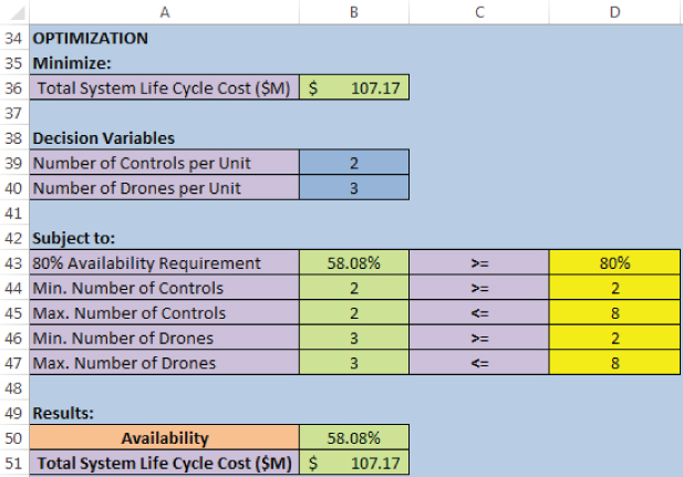
Figure 13.11 The “Decision Variables, Constraints, and Results” portion of the Control Panel tab
Figure 13.12 provides an example of the Calculations tab. It is used to calculate the value of Ao (Cell B11) that results from the values of the input and decision variables provided in the Control Tab.

Figure 13.12 The Calculations tab
Figure 13.13 provides an example of the summary-level portion of the Life Cycle Cost tab. The Life Cycle Cost tab contains values for all the life cycle model inputs (that were addressed in the Control Panel), intermediate cost calculations (in green), and the calculation of the total life cycle cost (Cell D7). Recall it is this value that is to be minimized. (The reader is referred to the online version of this book for color indication.)

Figure 13.13 The life cycle cost tab
Once all input parameters and decision variable values are specified, optimization can be performed to the model using Solver's Evolutionary Method. Figure 13.14 demonstrates how the Solver window is used to minimize the objective (the TSLCC in cell B36), over the range of decision variables (provided in cells B39 and B40), subject to the indicated constraints on Ao, Nc, and Nd in the Control Panel tab. Given these values one selects “Solve.”

Figure 13.14 Solver window
Figure 13.15 provides an example of how the “Decision Variables, Constraints and Results” portion of the Control Panel tab changes as a result of the optimization. We can see that the values in Nc and Nd (cells B39 and B40) are now populated with the decision variable solution (Nc = 7, Nd = 6), the resulting constraint-satisfying value for Ao (80.20%) populating cell B50, and minimum TSLCC that results ($111 M) in cell B51.

Figure 13.15 Optimization results
13.4.3 Discussion of the Optimization Model Results
The solution obtained in the previous section has an estimated TSLCC of $111 M which is ∼$7 M less than the solution obtained by hand in Section 13.3.3. We see that automated implementation of an optimization algorithm allows us to find more optimum solutions with much less effort than can be found using a manual search.
The automated search showed that it was far less expensive to adopt a design solution with additional control and drone elements, than it was to adopt the design with a greater maximum flight time. It should be noted that the solution might well change if one increases the number of units that are to be procured or other changes are made to either the availability model or the TSLCC model.
Figure 13.16 was obtained using the data tables constructed in the Control Panel tab of the Excel model described in the previous section. It indicates the availability/cost trade space associated with keeping Tmf = 4.0 h. It shows the cost associated with each of the 49 design solutions that resulted from taking values for Nc and Nd that increased incrementally from 2 to 8.26

Figure 13.16 Availability/TSLCC tradespace (Ttf = 4 h)
We can see from this graph that very little improvement in Ao is achieved by increasing Nd beyond about 6 or 7 or Nc beyond about 4.
13.4.4 Deterministic Sensitivity Analysis
Prior to performing a Monte Carlo analysis of a system, one should determine which uncertainties are likely to have the greatest effect on the metrics of interest. This is typically done by performing a single factor sensitivity analysis. In such analysis one first determines the (deterministic) “base” (expected) value for the metric of interest (in this case Ao) based on assigning “base” (expected) values to each of the input factors. One then systematically varies the value of each of the input factor from its “worst” value (i.e., the value that results in a lower Ao) to its “best” value (yielding a higher Ao), while holding all other inputs factors at their base values.
The Optimization Excel model developed in Section 13.4.2 may be used to perform such an analysis. Columns J, K, and L of the “Ao Input Parameters” portion of the Control Panel tab are used to specify the worst, base, and best values for each input factor. These values are then used to determine the resulting “swing” in the value of Ao that would result from such changes in input values (this is done in cells A55–D105). The results of such an analysis may be presented as a “Tornado Diagram.” Figure 13.17 provides an example of such a diagram that was obtained using the “optimum system design” of Nc = 7 and Nd = 6.

Figure 13.17 Tornado diagram for Nc = 7 and Nd = 6
This diagram provides a great deal of useful information. It tells us that uncertainties in Pap and postflight maintenance time are the greatest sources of uncertainty in the expected value of Ao (they can swing it by ∼9%–14% in either direction). It also shows that uncertainties MDTlog, Preflight Prep. Time, MTBCF1d, MTBCF1c, and MDT2c can result in Ao swings of about 1–8% in either direction. This implies that in developing a Monte Carlo model, one should certainly model the first two variables as random and possibly the next five as well. Since uncertainty in the remaining six variables has a relatively small impact on the value of Ao, they may be treated as constants (equal to their base values). Finally, the asymmetric nature of many of these uncertainties (there is greater “downside” impact than “upside” impact) may be expected to give rise to an “expected” Monte Carlo value of Ao that is lower than the “base” deterministic Ao. We will see that this is the case in the following section.
13.5 Monte Carlo Modeling
There are at least two different ways in which Monte Carlo modeling may be done to support the kind of sustainment analyses described in this chapter. The first approach is to develop a “Scenario/Mission-based” Monte Carlo simulation for system availability that models the takeoff, flight, landing, failure, and maintenance of each drone and the failing and replacement/repair of each control element over some time period of interest. Such a model could be used to validate the analytic model developed in Section 13.2, explore the implications of more realistic distributions for key parameters, explore transient (as opposed to steady-state) behavior, and get better feel for the day-to-day variability in system availability that one could expect to see. Such models are generally time-consuming to develop and are left as an exercise for the reader (see Exercise 2 at the end of this chapter).
The second approach is to use Monte Carlo simulation to develop a sense of the degree to which uncertainties in input factor values can yield uncertainties in model output metric values. It is this later approach that is considered in this section.
The models developed in the previous sections (except Section 13.4.4) did not address uncertainties in the ability to achieve designs or the values of various cost parameters. While such deterministic modeling is useful for establishing a modeling framework and for obtaining crude point solution “expected values” for important system metrics, it does not give one a sene of the uncertainty and risk associated with achieving those expected values. This section provides an example of how to develop Monte Carlo extensions to the deterministic availability optimization and cost models developed in Section 13.4 and illustrate how such extensions may be used to determine performance and cost risk. The model can be found in the file CH13 FMDS Monte Carlo Analysis.xlsx available online as supplementary material.
13.5.1 Input Probability Distributions for the Monte Carlo Model
Uncertainty can be incorporated into FMDS model by adding probabilistic distributions to lower level parameters. These are represented in the influence diagram in Section 13.1.1 by the parameters circled by an ellipse. By adding uncertainty to these parameters, the resulting availability value will differ from the one obtained through deterministic analysis. The degree of such variation is dependent on the probabilistic distributions assigned to each parameter. As discussed in Section 13.4.4, probabilistic distributions should be assigned only to those input parameters that have determined to have the greatest impact on the output metric of interest (i.e., the availability) through deterministic sensitivity analysis. For this reason, triangular distributions were added to the top seven uncertainties in Figure 13.17. Figure 13.18 illustrates the probability density function for the triangular distribution embedded to drone postflight maintenance time as an example of the added distributions using Palisade's @Risk package for Excel.

Figure 13.18 Postflight preparation time triangular distribution
The minimum, peak, and maximum values for postflight maintenance time (Tpfm) are 0.5, 1, 2 h respectively (from Figure 13.18). For this factor, the minimum value corresponds to the “best case,” that is, it results in a larger value for Ao.27 It should be noted that distribution is skewed toward higher values of Tpfm. As a result, the mean of the distribution is higher than the “peak” values. As such, one would expect that the resulting (Monte Carlo) mean value for Ao would be lower than the one predicted using the deterministic model.
13.5.2 Monte Carlo Simulation Results
Once all triangular distributions have been incorporated to low-level parameters, Monte Carlo simulation can be performed to obtain the expected system availability when uncertainty is present in the model. Figure 13.19 shows the cumulative density functions for 7 controls/6 drones, 8 controls/7 drones, and 5 controls/8 drones. Besides 7 controls/6 drones, these combinations were considered since they were the ones that approached the 80% requirement at the lowest TSLCC.

Figure 13.19 Cumulative density functions for control/drone combinations
The leftmost cumulative density function corresponds to the 7 controls/6 drones combination that resulted in the least expensive design that was able to meet the Ao ≥ 0.80 requirement. We see that in this case, the MC model provided a mean Aomc = 0.7716, which is lower than the Aod = 0.8020 obtained from the deterministic model in Section 14.4.2. In order to determine whether this is significant, we need to calculate the uncertainty in Aomc. The “Standard Error”(SE) provides a measure of this uncertainty. It is calculated from the standard deviation (SD) and number of runs (Nr) using:
Given this, one should technically report the value of the MC mean as:
Since the difference between Aomc and Aod is more than two standard errors, we can conclude that the difference is statistically significant. Generally, there are two potential sources for such differences. The first is skewness in the input distributions. The second is nonlinearity of the functions used to determine the value of the output value.
The cumulative probability distribution generated for Ao in Figure 13.19 may be used to determine the “confidence” that a given design will be able to meet its requirement. This permits us to perform the following confidence/design trade studies. As an example, in the Nc = 7, Nd = 6 case, we see that about a 68% of runs resulted in values of Ao less than 0.80, corresponding to a 32% confidence that the design will meet the requirement. If we increase Nc to 8 and Nd to 7, only about 48% of runs fall below Ao = 0.80, corresponding to a 52% confidence that this design will meet the requirement. Alternatively, if we decrease Nc to 5 and increase Nd to 8, only about 40% of runs fall below Ao = 0.80, corresponding to a 60% confidence that this design will meet the requirement.
13.5.3 Stochastic Sensitivity Analysis
The Monte Carlo simulation performed in the previous section also serves as a tool to conduct a stochastic sensitivity analysis for the optimal solution found in Section 13.4.3. Specifically, the most sensitive uncertainties determined from the deterministic sensitivity analysis in Section 13.4.4 can be analyzed to determine their respective contribution to the variability in system availability when probabilistic distributions are added. This can be done through @RISK's Change in output mean tornado diagram functionality as shown in Figure 13.20.

Figure 13.20 Tornado diagram for the FMDS system
This plot differs from the deterministic tornado diagram in that the lower (upper) values of Ao for each parameter are the mean of the 10% of Monte Carlo runs that had the worst (best) random values for that parameter. 28 The results of the stochastic tornado diagram display some important differences relative to its deterministic equivalent. First, we see that the expected (base) value has changed. Second, we see that there is a decrease in the maximum availability that could be possibly met when varying the most sensitive parameter (Prob. of Available Part). The deterministic sensitivity analysis indicated that the value of Ao could exceed 89% as shown in Figure 13.17, whereas Ao only reaches 84.94%. Third, the sensitivity bars associated with the stochastic diagram are more symmetric than those associated with the deterministic diagram. Finally, the stochastic analysis suggests there is a change in the order of most sensitive uncertainties. When stochastic analysis is performed, MTBCF1d moves from the fifth position in the order to the least sensitive parameter. Similarly, MDT2c moves from seventh position to the sixth most sensitive parameter. Post-flight maintenance time and MTBCF1c also change positions. One of the reasons for the changes in the magnitude and symmetry of the effects, and their order of importance, is that the stochastic analysis reflects the mathematical coupling between parameters, while the deterministic analysis does not.
13.6 Chapter Summary
The availability of a system is an important operational performance parameter. The associated reliability and maintainability requirements are major drivers of system's TSLCC, especially those associated with operations and support (which generally account for the majority of total life cycle cost). As such, it is important to have models that provide decision-makers information regarding the cost-effectiveness of different designs and different operational and maintenance concepts.
To this end, Section 13.2 developed a first-order performance model for the availability of the FMDS as a function of a variety of design, operational, and maintenance factors and demonstrated how such a model could be used to perform a variety of sensitivity and trade-off analyses related to system design and to associated operational and maintenance concepts.
Section 13.3 developed a first-order total life cycle cost model for the FMDS (with a special focus on life cycle O&S costs) within the context of standard DoD cost WBSs. It then demonstrated how to integrate the cost model with the performance model developed in Section 13.2 and how to use such an integrated cost–performance model to perform a cost-effectiveness trade-off analysis.
Section 13.4 demonstrated how one could develop an Excel model that employs an evolutionary optimization technique to find the lowest cost design solution that meets the system's availability and automatically generate a “cost-effectiveness” tradespace curve. It also showed how one could use a tornado diagram to determine which input factors have the greatest effect on a given output metric. We saw that this helped us identify the most important parameters to model as random variables in a Monte Carlo model and provided information that could be used to determine the shape of the associated random number generators.
Section 13.5 provided an example of how to develop a Monte Carlo extension to the deterministic availability model developed in Section 13.2 and how such a model can be used to determine the confidence that one may have that a given design will be able to meet its requirement. It also showed how one could perform a stochastic sensitivity analysis to determine the degree to which each input parameter affects the output metric, as the other parameters are varied stochastically.
The models developed in this chapter illustrate important modeling and trade-off analysis techniques and lessons. One of the most important lessons in modeling is that if one attempts to model everything, one will successfully model nothing. As such, this chapter demonstrated how to develop first-order models based on simplifying assumptions that may be used to provide a framework for initial studies and for elaboration, in spiral fashion, to develop more complicated models that incorporate fewer simplifying assumptions.
Other important “takeaways” from this chapter include the following:
- Cost-effectiveness trade studies provide information that is essential for many design decisions.
- Generally, a cost-effectiveness trade study requires the development of two types of models: (i) one or more system performance (system effectiveness) models and (ii) one or more cost models.
- One should develop a cost model that reflects how different design options will affect the TSLCC, not just the cost associated with one portion of the cycle (e.g., development or production).
- Performance models and LCC models permit one to structure the problem and guide the analysis. Even first-order (performance and life cycle cost) models can be complicated and require the use of many input parameters.
- As such, one should initially focus on identifying and modeling only the most important value functions and associated factors, relationships, and effects that affect them.
- Performance models and LCC models should be extensible so that they may be modified to address changes in simplifying assumptions and/or additional information that is uncovered during the course of the study.
- It is important to develop integrated performance and cost models so that one may observe how a change in a parameter value can simultaneously affect both the performance model (e.g., availability) and the life cycle cost model.
The purpose of this chapter is to illustrate techniques for developing models that can be used to perform RAM-related cost-effective trade studies and for performing such trade studies (not to provide a detailed trade study of a specific, real system). As such, the models are based on a variety of illustrative simplifying assumptions and make use of fictional data. The resulting modeling framework can then be extended to develop more detailed and accurate models for real systems, based on real data and fewer simplifying assumptions. The exercises at the end of this chapter provide the reader an opportunity to explore some of these extensions and a wider range of sensitivity and trade-off analyses than were covered in the chapter.
13.7 Key Terms
- Availability: the probability that a system or equipment, when used under stated conditions, will operate properly at any point in time.
- Complex Structure: a system composed of multiple instantiations of multiple types of elements that interact with one another, which differ significantly in their form and function. In addition, each element is characterized by multiple failure modes, a mixture of series and parallel reliability architectures, and load sharing.
- Cost Estimating Relationship: a mathematical function that indicates how a set of variables are related to one another. It is often obtained through regression analysis.
- Cost Model: a mathematical model that calculates the cost associated with some aspect of a system based on the input values of some set of factors.
- Critical Failure: a failure that requires an element to abort its mission and seek immediate repair.
- Cold Standby: the case in which a “standby elements” does not become active until the active element fails. There is generally a short system “downtime” associated with this replacement.
- Development Cost: the total cost associated with designing, production, and testing of system prototypes and/or engineering development models, as well as that associated with requirements development, technology development, system analysis, and system trade studies.
- Deterministic Model: a model in which none of the variables are random.
- Downtime: the time a system or element is inoperable following a failure or associated with a scheduled maintenance. Generally, it includes the time to obtain the parts required to repair the item, the time required to repair it, and any additional time required to return it to service. In the case of a standby element, it consists of the time between when the active element fails and the standby element is able to take its place and the system is able to resume operation.
- Influence Diagram: a diagram that consists of decision nodes, uncertainty nodes, and value nodes connected by directional arcs that indicate that the behavior/value of the source node influences the behavior/value of the end node.
- Integrated Performance/Cost Model: a mathematical model that calculates the cost of some aspect of a system and the performance of the system (with respect to one or more response variables of interest) based input values for some set of cost and performance factors.
- k-Out-of-n Cold Standby System: a parallel structure composed of n elements in which k elements must operate simultaneously for the system to be operational and the remaining n–k elements are nonoperating (cold) “standby elements.” If one of the k operating elements experiences a failure, it is switched off and one of the standby elements takes its place (after a short replacement downtime).
- Maintainability: the probability that an item will be retained in or restored to a specified condition in a given period of time, when maintenance is performed in accordance with prescribed procedures and resources.
- Markov Process: a system that is characterized by a set of states and a set of transition probabilities that depend only on the current state of the system.
- Mean Downtime: the average downtime experienced by a system or element.
- Mean Time Between Critical Failures (MTBCF): the average time that a system or elements operates without experiencing a critical failure (i.e., the average operating time between critical failures).
- Monte Carlo Simulation: a simulation that makes use of repeated random sampling of one or more random variables in order to obtain numerical results. Within the context of this chapter, the term is used to refer to “Scenario/Mission-based” Monte Carlo simulations and “Uncertainty Analysis” Monte Carlo simulations.
- Operational Availability: the probability that a system or equipment, when used under stated conditions in an actual operational environment, will operate satisfactorily when called upon.
- Operations and Support (O&S) Cost: the total cost incurred from system deployment through end of system operations. It includes the costs of operating, maintaining, and supporting a fielded system.
- Performance Model: a mathematical model that estimates the performance of a system with respect to one or more response variables based on the input values of some set of factors.
- Procurement Cost: the total cost of producing and deploying all of the units that make up the system over its operating life.
- Reliability: the probability that a system or product [element/item/service] will perform in a satisfactory manner for a given period of time, when used under specified operating conditions.
- Reliability Block Diagram: a diagram that identifies how the reliability of different elements contributes to the reliability of a system. Components are drawn as being in series or parallel configurations.
- Retirement/Disposal Cost: the cost associated with retirement and disposal of the system, including the cost of disposing of hazardous materials.
- Sensitivity Analysis: a type of trade-off analysis in which one evaluates the degree to which a change in one or more input factors affects the value of an output metric.
- Standby Element: a redundant element that is able to replace an active element that is required for system operation, if the active element fails.
- Stochastic Model: a model in which one or more variables are random.
- Structure: a collection of elements connected to one another in a series and/or parallel architecture.
- Total Life Cycle Cost: the total cost of a system over its entire life cycle, from conception, through development, production, operations and maintenance, and retirement/disposal.
- Tornado Diagram: a diagram that indicates the degree to which an output metric varies as one changes the value of input parameters from their lowest to their highest values. The input variables that lead to the greatest change in output metrics are placed at the top, and those that lead to the smallest variation are placed on the bottom.
13.8 Exercises
- 13.1 Construct the analytical availability model provided in Figure 13.5 using Excel.
- a. Reproduce the results.
- b. Develop a graph showing how availability of the system varies the reliability of the control element (MTBCF1c) from 50 to 200 h in 25 h steps.
- c. Develop a graph showing how the availability of the system varies as the reliability of drone element (MTBCF1d) from 20 to 100 h in 20 h steps.
- d. How would one determine whether it is better to focus development effort on improving control element or drone element reliability (a design decision)?
- e. Develop a graph showing how the availability of the system varies as the logistics downtime (MDTlog) for the drone element increases from 10 to 80 h in 10 h steps. Note that this represents decrease in maintainability.
- f. Develop a graph showing how the availability of the system varies as the preflight preparation time (Tpfp) for the drone element increases from 0.2 to 1.0 h in 0.2 h steps. Note that this also represents decrease in maintainability.
- g. Does it make more sense to focus on decreasing the logistics downtime or the preflight preparation time (a maintenance concept decision)? Explain.
- h. How would one determine whether it is better to focus improving design (MTBCF) or the maintenance concept (MDTlog or Tpfp)? Note this is a decision regarding a trade-off between design and maintenance concept.
- i. Develop a graph showing how the availability of the system changes as one increases the number of drone elements in a system from 2 to 5.
- j. Under what conditions would one want to increase the number of drones in a unit (i.e., system architecture), as opposed to increasing element reliability (a change in design)?
- k. Develop a graph showing how the availability of the system changes as one increases the maximum flight time of the drone element from 3 to 7 h in 1 h steps (a change in design and possibly operational concept).
- l. Under what conditions would it make sense to trade an increase in maximum flight time for a decrease in number of drone elements per unit?
- m. Develop a graph showing how the availability of the system changes as one increases the time to station of the drone element from 0.1 to 0.5 h in 0.1 h steps (a change in operational concept).
- 13.2 Develop a “Scenario/Mission-based” Monte Carlo simulation for the FMDS using the parameter values provided in Table 13.3. In this case, one should model the takeoff, flight, landing, failure, and maintenance of each drone and the failings and replacement/repair of each control element over some time period of interest. This will include the generation of random failure times and maintenance times and the control logic that will cause one drone to take off to replace a drone returning to base (scheduled or unscheduled).
- a. How long did it take you to develop the analytical model used in Problem 1?
- b. How long did it take you to develop this working Monte Carlo model?
- c. Run the MC simulation until the mean value for the availability “settles down” (does not change by more than about 10%).
- For what value of system time did this occur?
- What value of Ao was obtained?
- d. How does this result compare to the result obtained using the analytical model? If there are differences, what are some likely explanations of the differences?
- e. How long did you have to wait to obtain the Monte Carlo result? How long did it take to get an answer using the analytical model?
- f. Perform 100 repetitions of this Monte Carlo simulation and determine the Mean Availability and the standard error.
- g. How do these results differ from those obtained in c? Which is more likely the true mean? Explain.
- h. How do the results in f. differ from the analytical model? Are the differences significant? Why or why not?
- i. If the differences found in h. are significant:
- Identify the likely sources of these differences.
- Indicate which result is more likely to be observed in a real operating system. Explain your answer.
- j. Under what conditions would you want to use the analytical model?
- k. Under what conditions would you want to use the Monte Carlo simulation?
- l. How might one use the two types of models in a synergetic manner?
- 13.3 Explore the cost-effectiveness of reducing the MDTi associated with Effective Drone Failures with no standby available.
- 13.4 Explore the cost-effectiveness of increasing the MTBF for the control element (see Section 13.2). What costs would be affected by doing this? Develop a model for determining these costs.
- 13.5 Assuming a constant inflation rate of 2% per year, calculate the total O&S cost of the system described in Table 13.11 in “then-year” dollars.
- 13.6 Assuming a discount rate of 3%, calculate the net present value of the O&S cost of the system described in Table 13.11. (Hint: see net present value analysis is Chapter 4.)
- 13.7 What is the difference between the O&S cost calculated in “current-year” dollars and “then-year” dollars and net present value?
- 13.8 Suppose you are uncertain about the value of the following parameters, but expect them to be in the ranges indicated as follows:
Parameter Min Max System life 15 yr 30 yr Operators per unit 4 6 Annual cost per personnel $80,000/per $130,000/per Operations cost/hour $30/yr $60/hr Mean time between critical failures (drone) 30 h 80 h Ratio of drone failures requiring part replacements to critical failures 1 10 Mean cost to replace a drone part $250/part $500/part - a. Develop a Pareto Chart that shows the degree to which uncertainty in these values can affect the Total O&S Cost.
- b. Which of these would it make the most sense to use in Monte Carlo cost simulation? Why?
- 13.9 Develop a Monte Carlo simulation for the cost model provided in Table 13.11. Assume a triangular distribution with the following properties, for the following parameters:
Parameter Min Most Likely Max Operations cost/hour $30/yr $40/h $60/h Mean time between critical failures (drone) 30 h 50 h 80 h Ratio of drone failures requiring part replacements to critical failures 1 3.0 10 - a. Find the mean Total O&S Cost.
- b. Find the standard deviation associated with this mean.
- c. How many runs of the Monte Carlo simulation were required to get an appropriate mean and standard deviation? How did you determine this?
- d. What is the 80% confidence Total O&S Cost for this system?
- 13.10 Develop a TSLCC model for a system of interest to you.
- a. Determine the TSLCC in “current-year” dollars.
- b. Determine the TSLCC in “then-year” dollars.
- c. Perform a sensitivity study with respect to one or more input parameters.
- d. Perform a trade-off study with respect to one or more input parameters.
- e. Based on your trade-off study results, provide a recommendation as to what the program should do with respect to those values and the rationale for your recommendation.
References
- Amari, S. (2012) Reliability of k-out-of-n standby systems with gamma distributions. IEEE Transactions on Reliability.
- Amari, S., Zuo, M.J., and Dill, G. (2008) O(kn) Algorithm for analyzing repairable and non-repairable k-out-of-n: G systems, in Handbook of Performability Engineering (ed. K.B. Misra), Springer, pp. 309–320.
- Birolini, A. (2007) Reliability Engineering: Theory and Practice, 5th edn, Springer.
- Blanchard, B. and Fabrycky, W. (2010) Systems Engineering and Analysis, 5th edn, Pearson.
- Boddu, P. and Xing, L. (2012) Redundancy Allocation for k-out-of-n:G systems with mixed spare types. IEEE Transactions on Reliability.
- CJCSI 3170.01I (2012) Joint Capabilities Integration and Development System (JCIDS).
- Defense, D. o (2014) Operating and Support Cost-Estimating Guide. Chapter 6, Office of the Secretary of Defense Cost Assesment and Program Evaluation.
- DoD Instruction 5000.02 (2015) Operation of the Defense Acquisition System.
- INCOSE (2015) Systems Engineering Handbook: A Guide for System Life Cycle Processes and Activities, 4th edn, Wiley.
- Jacob, D. and Amari, S. (2005) Analysis of complex repairable systems. IEEE Transactions on Reliability.
- Kuo, W. and Zuo, M. (2003) Optimal Reliability Modeling: Principles and Applications, Wiley.
- Lad, B., Kulkarni, M., and Misra, K. (2008) Optimal reliability design of a system, in Handbook of Performability Engineering, Springer.
- Morrison, M. and Munshi, S. (1981) Availability of a v-out-of-m+r:G system. IEEE Systems Transactions on Reliability, R-30 (2), 200–201.
- Sandler, G. (1963) System Reliability Engineering, Prentice Hall.
- van Gemund, A. and Reijns, G. (2012) Reliability of k-out-of-n systems with single cold standby using Pearson distributions. IEEE Transactions on Reliability.
- Wang, W. and Loman, J. (2012) Reliability/availability of k-out-of-n systems with m cold standby units. Proceedings of Annual Reliability and Maintainability XE “Maintainability” Symposium.
- Zuo, M., Huang, J., and Kuo, W. (2003) Multi-state k-out-of-n systems, in Handbook of Reliability Engineering (ed. H. Pham), Springer.