
Chapter 12
Exploring the Design Space
Clifford Whitcomb and Paul Beery
Systems Engineering Department, Naval Postgraduate School, Monterey, CA, USA
Design is not just what it looks like and feels like. Design is how it works.
(Steve Jobs)
12.1 Introduction
This chapter presents three examples for application of the design of experiments (DOEs) method to systems design. There are two examples from industry: a liftboat example from the offshore oil industry and a cruise ship design. The liftboat uses a fractional factorial design, while the cruise ship uses a Taguchi design. These designs are useful in very early design stages due to the minimal number of points needed. They are useful when information or data is limited or when design synthesis tools are not readily available to develop sets of design variants for complicated systems. Taguchi designs make it possible to explicitly examine “noise” while not including those factors in the design (thereby increasing the number of runs required). Taguchi designs are also resolution III and have interaction effects confounded with main effects, which limit the utility of the results. The third example is for a design of a NATO naval surface combatant ship. This NATO ship example uses a Box–Behnken design. Ship design synthesis tools for naval combatant ships are readily accessible by naval architects, so the design points needed for the DOE method are more readily created. This allows for the use of DOEs that typically require more design points, such as Box–Behnken or Central Composite Designs with several variables as factors. These Box–Behnken and Central Composite Designs have resolutions IV and higher, so have fewer confounded effects. This provides for design trade-offs with fewer concerns about interaction effects potentially interfering with design conclusions based on analysis of results.
12.2 Example 1: Liftboat
With the current desire to expand offshore drilling for petroleum resources, there has been an expanding market for a capability to maintain offshore rigs. Liftboats provide this capability, especially in the Gulf of Mexico. A liftboat is designed to be a self-elevating, self-propelled vessel with at least one crane and deck space that is open enough to serve multiple purposes. A liftboat is not a conventional jack-up boat or a drilling rig. Liftboats carry the kind of equipment needed to perform platform maintenance, fracking, sand blasting, pipe-laying, and so on. A list of liftboats is available at http://www.shipbuildinghistory.com/history/merchantships/postwwii/liftboats.htm.
Liftboats are classed by leg length. Design considerations allow for leg penetration into the sea bottom, the size of the air gap between the water surface and the vessel hull, and a leg reserve length, which are all part of developing a desired water-depth capability. The operational water depth drives the profits for companies that operate them. In general, the deeper a liftboat can operate, the more profits for the owners. Operational water depths for these vessels approach 300 ft, with leg lengths of over 300 now feasible. As far as the liftboat subsystems are concerned, the legs are the critical subsystem, from both the customer and shipbuilder perspectives. The legs are shown on a liftboat docked in a shipyard in Figure 12.1.
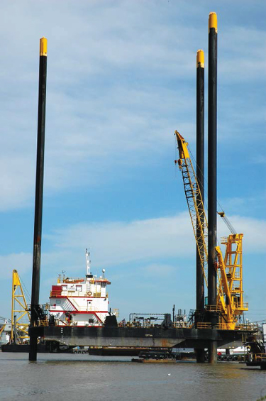
Figure 12.1 Liftboat docked at the Bollinger Shipyard in Louisiana (Courtesy of Cliff Whitcomb)
The longer leg lengths needed to provide deeper water capability results in heavier legs, which reduces the lifting capacity of the vessels, as well as reducing the stability both in getting the liftboat to the operational area, and when in operation. In order to look for possible design variations, several leg designs have been attempted with different types of leg internal structures. Figures 12.2 and 12.3 show two typical leg designs of leg structural internals for liftboats. The leg shown in Figure 12.2 uses plate internals, and Figure 12.3 shows a leg with “ladder-” or “lattice-”type internals. The legs are made of high-strength steel, and production is challenging in accomplishing the welding of the internals. Leg construction alternatives that result in a lower displacement are desired for a resulting design, as the lift weight is reduced.
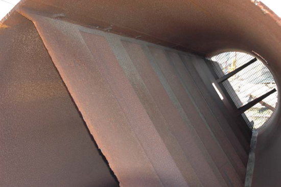
Figure 12.2 Liftboat leg internals using a plate construction (Courtesy of Cliff Whitcomb)
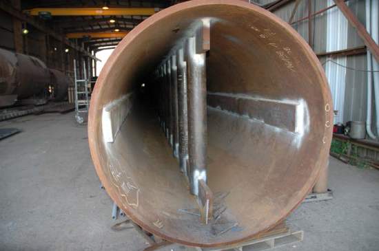
Figure 12.3 Liftboat leg internals using a lattice construction (Courtesy of Cliff Whitcomb)
12.2.1 Liftboat Fractional Factorial Design of Experiments
To explore the possibility of constructing liftboats with deeper water capability, a DOE was defined using a two-level five-factor fractional factorial design. This notional example DOE was used to study the design possibilities for reaching deeper operational water depths using various factors of leg diameters, lengths, and thicknesses and responses of displacement and lift weight. The leg internals are not used in this first trade-off, as they would be designed after the overall liftboat study of displacement and lift weight based on leg diameter, length, and thickness. The results were analyzed using regression analysis using JMP statistical analysis software. The fractional factorial was chosen as the ability to synthesize liftboat designs to cover the design space was limited by the ability of the existing ship design synthesis tools to formulate liftboat designs, from both a technical aspect and the amount of time needed to design ship alternatives. The resulting set of liftboats for the analysis is shown in Table 12.1, which is a condensed version of the full data table limited to three factors and two responses (the full data table is available on the textbook website).
Table 12.1 Fractional Factorial Design for Liftboat
| Pattern | Leg Length | Leg Diameter | Leg Thickness | Displacement | Lift Weight |
| ++++++ | 445 | 9 | 3 | 1000 | 3840 |
| +−+−+− | 445 | 9 | 0.757 | 640 | 240 |
| ++−+−− | 445 | 3 | 0.757 | 700 | 2000 |
| +−++−+ | 445 | 3 | 3 | 550 | 500 |
| −+−+−+ | 130 | 3 | 3 | 300 | 1200 |
| −++−−+ | 130 | 3 | 3 | 300 | 1200 |
| +−−−−+ | 445 | 3 | 3 | 600 | 250 |
| −−++−− | 130 | 3 | 0.757 | 210 | 300 |
| ++−−++ | 445 | 9 | 3 | 1000 | 3840 |
| +−−++− | 445 | 9 | 0.757 | 640 | 240 |
| −−+−++ | 130 | 9 | 3 | 300 | 3500 |
| −−−+++ | 130 | 9 | 3 | 600 | 5200 |
| +++−−− | 445 | 3 | 0.757 | 1050 | 3000 |
| −+−−+− | 130 | 9 | 0.757 | 300 | 1200 |
For displacement, the leg length is found using JMP to be statistically significant, with a p-value of 0.0013. For lift weight, both leg diameter, p-value of 0.0142, and leg thickness, p-value of 0.0209, were found to be statistically significant in the JMP analysis. Figure 12.4 presents an example leg configuration in terms of leg length, leg diameter, and leg thickness. Recall that operating depths of over 300 ft are desirable; accordingly, the leg length is fixed as 335 ft, the leg diameter is set at 9 ft, and the leg thickness is set at 1.875 ft. More detailed examination of this complete trade-off space is required to investigate the appropriateness of the values for leg diameter and leg thickness.
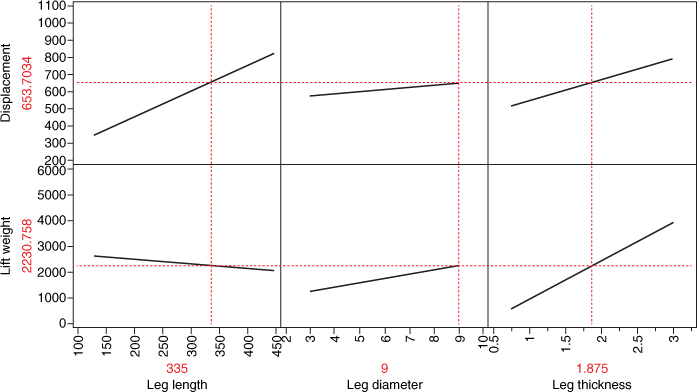
Figure 12.4 Liftboat tradespace for the two responses with respect to the three factors
12.2.2 Liftboat Design Trade-Off Space
A potential desired design for a liftboat to achieve 335 ft leg length, indicated in Figure 12.4 by the lines on the x and y axes, shows a predicted displacement of 654 Ltons and a lift weight of 2,231,000 lb. Figure 12.5 shows a different view of the variable relationships in the form of a “cut” through the trade-off space. The graph shows displacement and lift weight as a function of leg diameter and leg length. Constraint for the designer's desired limit for minimum lift weight is set to 2,200,000 lb and the limit for maximum displacement is set to 675 Ltons. The gray shaded areas are regions that do not meet the constraints where the shaded on the left hand side of the graph corresponds to the leg length and leg diameter combinations that do not satisfy the lift weight constraint and the region shaded in the upper portion of the graph corresponds to the combinations that do not satisfy the displacement constraint. The white, unshaded region is the feasible trade-off space. The crosshairs on the right-hand side of the plot are set to a leg diameter of 9 ft and a leg length of 335 ft based on the values chosen in Figure 12.4. Further investigation of the trade-off space, with the leg thickness set to 1.875 inches, shows that the projected design appears feasible, as it is within the white space on the graph shown in Figure 12.5.
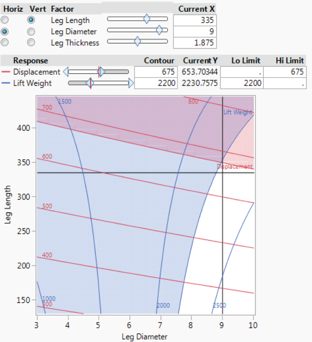
Figure 12.5 Liftboat design tradespace of displacement and lift weight versus leg length and leg diameter, at a leg thickness of 1.875 in
A quick investigation of existing liftboat designs reveals an existing liftboat, the Robert, that has a leg length of 335 ft, a leg diameter of 9.5 ft, a leg thickness of 1.875 in., with a displacement of 500 Ltons, a maximum water depth of operation at 280 ft, and a lift weight of 1,500,000 lb. Although the Robert's actual lift weight exceeds the constraint associated with this example trade-off, it is a reasonable choice to use for a quick check to verify the output of the liftboat design model as there are a very limited number of existing liftboat designs. The Robert is within the feasible region limit with respect to displacement. A brief study of the predicted design, based on the liftboat model, and an actual design, the Robert, can be accomplished by performing an uncertainty analysis.
12.2.3 Liftboat Uncertainty Analysis
To investigate the difference between the predicted result and the existing liftboat, a simulation with 5000 data points was performed using JMP to study the distribution of possible displacements in the model. The distribution, Figure 12.6, shows that the model has a mean of 655 Ltons and a standard deviation of 160 Ltons. The model shows a wide variability in the output. This is not surprising as there were few data points for this rough model. If a smaller variation about the mean were desired before using the model for decision-making, more time and effort would have to be put into developing more ship variants or collecting more actual ship data points design to attempt to reduce the variation and improve the prediction capability.
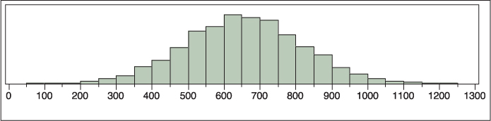
Figure 12.6 Distribution of liftboat model displacement outputs for N = 5000
12.2.4 Liftboat Example Summary
This example shows that DOE can be used to define the test points for a model of a liftboat before deciding on the detailed design for construction. The results of model analysis of the test points specified by the DOE can be used as a surrogate for available design tools when data, information, and design tools are limited or not available. The tradespace is then used to investigate the design possibilities, including using uncertainty analysis to further study the resulting liftboat design trade-off space.
12.3 Example 2: Cruise Ship Design
Traditionally, cruise ship design has been undertaken without consideration of system trade-offs. The two most important characteristics in designing a cruise ship are the economics, such as acquisition cost, profitability, operational cost, and the comfort of the cruise experience (Katsoufis, 2006). The naval architecture technical variable details of the ship characteristics are typically not as important as these business variables to the decision-makers. The trade-off is set up using a set of plots that show how the business variables are related to these technical variables.
12.3.1 Cruise Ship Taguchi Design of Experiments
In order to study the ramifications of early design decisions, a Taguchi screening experiment was performed on a notional cruise ship design. A set of eight factors was chosen to vary the technical aspects of the ship design, and three responses were selected to study their impact on the possible outcomes. The three responses are related to economic aspects are the ones used for decision-making. The fourth, the beam of the ship, is included since the beam can be limiting for transport through various canals, such as the Panama Canal. A Taguchi L18 design was selected for the experiment, Table 12.2.
Table 12.2 Cruise Ship Taguchi L18 Experimental Design
| Pattern | Passenger Capacity | Operational Range | Days of Stores | Propulsion Type | Number of Propulsors | Number of Engines | Brand Quality | Power Plant Type | Revenue | Acquisition Cost | Operating Cost | Beam |
| −−−−−−++ | 1,000 | 4,000 | 10 | Pod | 2 | 2 | Ultra | Diesel | 6,828 | 914 | 3,493 | 92 |
| +−−++−−0 | 3,000 | 4,000 | 10 | Screw | 4 | 2 | Budget | Combined | 12,049 | 1,590 | 5,655 | 118 |
| −−++−−0- | 1,000 | 4,000 | 20 | Screw | 2 | 2 | Premium | Gas turbine | 5,342 | 884 | 3,747 | 90 |
| ++++++++ | 3,000 | 8,000 | 20 | Screw | 4 | 4 | Ultra | Diesel | 20,483 | 2,115 | 7,816 | 137 |
| −++−−+−0 | 1,000 | 8,000 | 20 | Pod | 2 | 4 | Budget | Combined | 4,017 | 730 | 2,784 | 83 |
| +−+−+−0+ | 3,000 | 4,000 | 20 | Pod | 4 | 2 | Premium | Diesel | 16,025 | 1,914 | 6,837 | 130 |
| ++−+−−00 | 3,000 | 8,000 | 10 | Screw | 2 | 2 | Premium | Combined | 16,025 | 1,935 | 6,976 | 130 |
| +++−−−−− | 3,000 | 8,000 | 20 | Pod | 2 | 2 | Budget | Gas turbine | 12,049 | 1,577 | 6,267 | 118 |
| −−+−++00 | 1,000 | 4,000 | 20 | Pod | 4 | 4 | Premium | Combined | 5,342 | 857 | 3,241 | 90 |
| −+−+−+0+ | 1,000 | 8,000 | 10 | Screw | 2 | 4 | Premium | Diesel | 5,342 | 879 | 3,268 | 90 |
| +++++++0 | 3,000 | 8,000 | 20 | Screw | 4 | 4 | Ultra | Combined | 20,483 | 2,112 | 7,914 | 137 |
| −−−−−−+0 | 1,000 | 4,000 | 10 | Pod | 2 | 2 | Ultra | Combined | 6,828 | 973 | 3,688 | 96 |
| ++−−++0− | 3,000 | 8,000 | 10 | Pod | 4 | 4 | Premium | Gas turbine | 16,025 | 1,899 | 7,658 | 130 |
| +−++−+−+ | 3,000 | 4,000 | 20 | Screw | 2 | 4 | Budget | Diesel | 12,049 | 1,620 | 5,669 | 119 |
| −++++−+− | 1,000 | 8,000 | 20 | Screw | 4 | 2 | Ultra | Gas turbine | 6,828 | 1,033 | 4,366 | 99 |
| −+−−+−−+ | 1,000 | 8,000 | 10 | Pod | 4 | 2 | Budget | Diesel | 4,017 | 803 | 2,972 | 88 |
| −−−+++−− | 1,000 | 4,000 | 10 | Screw | 4 | 4 | Budget | Gas turbine | 4,017 | 785 | 3,351 | 86 |
| +−−−−++− | 3,000 | 4,000 | 10 | Pod | 2 | 4 | Ultra | Gas turbine | 20,483 | 2,085 | 8,615 | 135 |
12.3.2 Cruise Ship Design Trade-Off Space
The cruise ship L18 point designs shown in Table 12.2 were synthesized using a Microsoft Excel spreadsheet model provided on the textbook website. The Microsoft Excel spreadsheet was used to synthesize the ships, while JMP provided the DOE and resulting statistical analysis. The results were analyzed using JMP. The JMP results are shown in Figure 12.7 for the design point with the highest revenue.
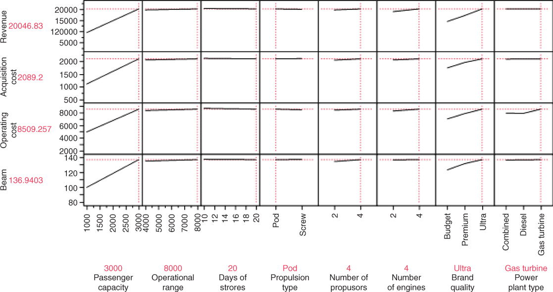
Figure 12.7 Trade-off space for cruise ships with variables set to the point with the highest revenue
The design space can be used to vary the factors to study the possibilities for different ship characteristics, such as number of passengers, propulsion type, power plant, and number of propulsors, and the range of possibilities for costs and revenue, within desired beam restrictions. The technical variable factors on the x-axes of Figure 12.7 can be set interactively in JMP, and the resulting business variable responses on the y-axes. The results show that five factors (operational range, days of stores, propulsion type, number of propulsors, and number of engines) have little or no impact on any of the MOEs that are the primary concern of the stakeholders. These do, however, maintain a link to the variables that the shipbuilders are primarily concerned with, so they are valuable to maintain an ability to discuss the ship characteristics among all stakeholders. The ship characteristics technical variables are set in Figure 12.7 to indicate the maximum revenue, while showing the ship beam in case this becomes an important consideration for passage through canals and other restricted waterways.
The design space can also be explored using the trade-off approach employed for the liftboat example. Figure 12.8 shows revenue, acquisition cost, operating cost, and beam as a function of passenger capacity and brand quality. A $10,000 minimum constraint is set for the Revenue at $10,000, a $1500 maximum constraint is set for the acquisition cost, a $5600 maximum constraint is set for the operating cost, and a 120 ft maximum constraint is set for the beam.
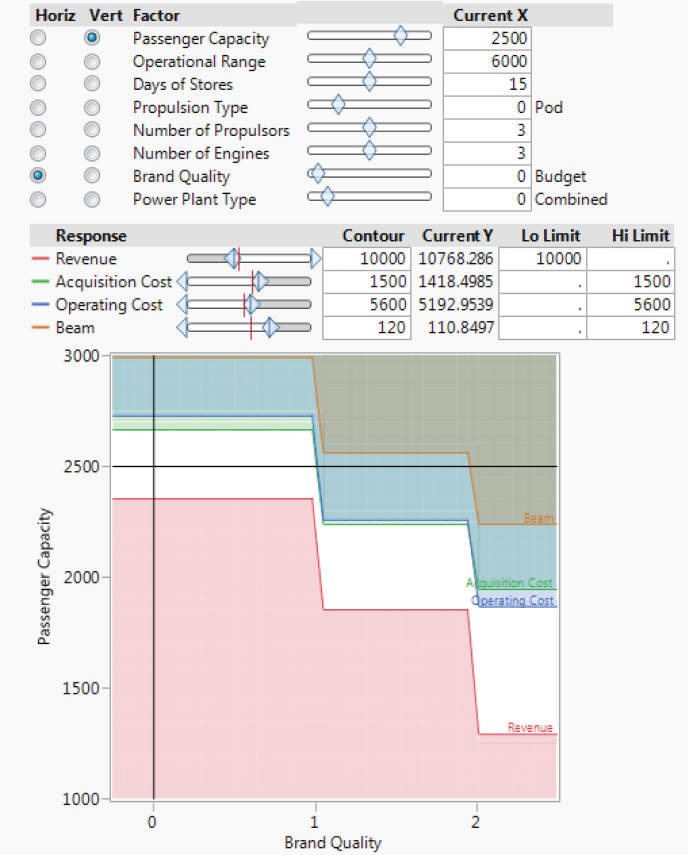
Figure 12.8 Cruise ship design tradespace of revenue, acquisition cost, operating cost, and beam versus passenger capacity and brand quality
The gray shaded areas correspond to the regions of the design space that do not meet the constraints (where referring to the right hand side of the graph where labels for the respective shaded regions are located the region corresponds to combinations that do not satisfy the revenue constraint, the shaded region just above the white region corresponds to operating cost, the next region up corresponds to the acquisition cost, and top-most shaded region corresponds to the beam). Note that the white, feasible region suggests that as the brand quality Increases, fewer passengers can be included in the ship. Currently, Figure 12.8 identifies a ship configuration with a budget brand quality and 2500 passengers as a feasible ship configuration. Note that the size of the feasible region will be reduced if the constraints are altered (Figure 12.9 presents an example).
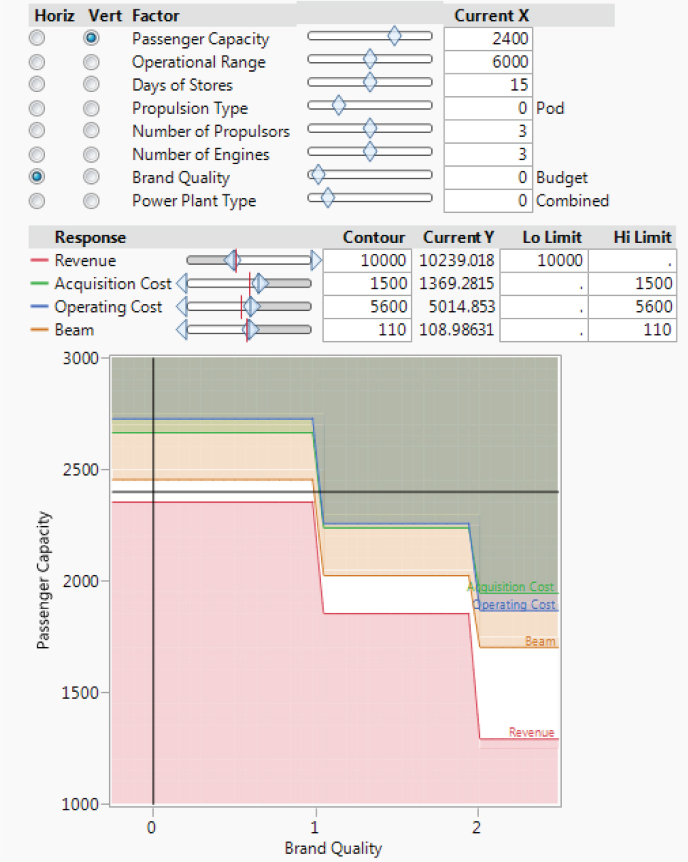
Figure 12.9 Cruise ship design tradespace of revenue, acquisition cost, operating cost, and beam versus passenger capacity and brand quality
Figure 12.9 shows the impact of a reduction in the allowable ship beam (note that it has been reduced from 120 ft in Figure 12.8 to 110 ft in Figure 12.9). This has rendered the previous ship configuration of 2500 passengers with a budget brand quality infeasible. Now it is only possible to accommodate 2400 passengers, even with a budget brand quality, due to the reduction in acceptable ship beam.
12.3.3 Cruise Ship Example Summary
This example shows a more basic trade-off structure where technical variables can be set to indicate the levels of business variable outcomes. The technical variables summarize the various ship variant alternatives that can be designed in order to meet desired business goals, while simultaneously checking a technical variable that might constrain operations in some desired concepts of operation.
12.4 Example 3: NATO Naval Surface Combatant Ship
NATO has planned a surface force concept to enable effective combat in littoral areas (NATO, 2004). The ship is envisioned as an integrated system-of-systems made up of sensors, decision aids, weapons and related support systems as part of a comprehensive maritime-based network. The combined capabilities of this surface strike force (SSF) concept will result in an integrated, multi-dimensional operational capability through which the joint force commander can both project power and protect joint forces from the sea.
In partial support of the overall SSF, a particular operations concept (OpsCon) is envisioned based on guidance for a series of flexible mission combatants, dubbed the flexible surface strike force (FSSF), which is to operate in littoral areas, and provide robust antiair warfare (AAW) self-defense, power projection ashore using gunfire support (GFS) and strike (STK), antisubmarine warfare (ASW), and antisurface warfare (ASUW). The FSSF must operate in conjunction with Aegis ships both as a net-centric asset and in independent operations. It must be capable of performing unobtrusive peacetime presence missions in an area of hostility and immediately respond to escalating crisis and regional conflict. The ship is likely to be forward deployed in peacetime, conducting extended cruises to sensitive littoral regions. Small crew size and limited logistics requirements will facilitate efficient forward deployment.
The FSSF will be among the first naval forces present in a region. It will perform detailed reconnaissance of surface and subsurface topography and the activities of potentially hostile forces. As hostilities intensify, the FSSF may be required to perform preemptive strike, lay mines, and conduct preassault shore bombardment. The FSSF may fall back to escort Amphibious Readiness Groups (ARG), mine counter measure (MCM) groups, or replenishment groups. It will continue to escort these groups or operate independently throughout the course of the conflict, providing flexible and robust ASW, ASUW, and STK capabilities as required. Although AAW emphasis will be on unit self-defense, some local area AAW defense capability will be required, particularly in cooperative engagement. As a conflict proceeds to conclusion, the FSSF will continue to monitor all threats. The FSSF may likely be the first to arrive and last to leave the conflict area. A notional ship design example is shown in Figure 12.10.
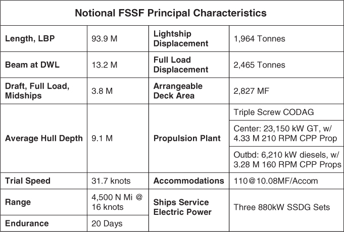
Figure 12.10 Notional FSSF ship design (Source: NATO. Reproduced with permission of NATO)
The FSSF is envisioned to be part of a NATO developed and deployed force. A reference study, the NATO NAVAL GROUP 6 SPECIALIST TEAM ON SMALL SHIP DESIGN NATO/PfP Working Paper on Small Ship Design, May 2004, is used as a basis for this example of design and acquisition of potential Offshore Patrol Vehicle (OPV) and Small Littoral Combatant (SLC) platforms. These platforms comprise the ships in the FSSF. The primary vessels to be procured as part of the initial effort are the corvette ships, with displacement of approximately 2000 Ltons.
12.4.1 NATO Surface Combatant Ship Stakeholder Need
The first step in this project is to determine the high-level stakeholder needs and requirements. Based on the NATO report, the stakeholder needs for this example are listed in Table 12.3.
Table 12.3 Stakeholder Needs for an FSSF
| FSSF Stakeholder Need |
| Information gathering |
| Protect sea lines of communications (SLOC) |
| Protection of high-value units |
| Embargoes and sanctions |
| Amphibious operations |
| Neutralize naval forces |
| JTF campaign |
| Support operations |
| Mobile capability |
| Independent operation capability |
| Flexible capability |
Understanding the priorities for these stakeholder needs is useful to accomplish a decision analysis. Using value functions, the stakeholders were found to have priorities as shown in Table 12.4.
Table 12.4 Prioritized Stakeholder Needs
| FSSF Stakeholder Need | Priority Weight |
| Information gathering | 0.05 |
| Protect sea lines of communications (SLOC) | 0.17 |
| Protection of high-value units | 0.17 |
| Embargoes & sanctions | 0.02 |
| Amphibious operations | 0.17 |
| Neutralize naval forces | 0.17 |
| JTF campaign | 0.09 |
| Support operations | 0.02 |
| Mobile capability | 0.03 |
| Independent operation capability | 0.02 |
| Flexible capability | 0.09 |
Next, the stakeholder value function curves for each of the needs were determined, with the results shown in Figure 12.11.
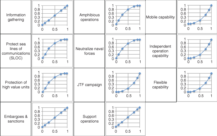
Figure 12.11 Stakeholder value functions for the various high-level needs
The individual value functions were rolled up into an alternative value, labeled in this case as Overall Measure of Effectiveness (OMOE), by multiplying the value for each need as indicated in the design outcome by the priority weight for each respective need (see Chapter 2 for further discussion of the additive value model).
12.4.2 NATO Surface Combatant Ship Box–Behnken Design of Experiments
In order to study the possibility for surface combatant ships that might meet the mission requirements, a DOE is conducted. The DOE used is a Box–Behnken design, with four factors at three levels, summarized in Table 12.5.
Table 12.5 DOE Data Table for FSSF Surface Combatant
| Pattern | Factors | Responses | |||||
| Speed (knot) | Range (nm) | Payload (Ltons) | Margin (%) | Cost (M$) | OMOE | Displacement (Ltons) | |
| 0+−0 | 30 | 6000 | 250 | 7.5 | 353.4 | 0.1776 | 2299.3 |
| +0−0 | 34 | 4500 | 250 | 7.5 | 415.2 | 0.1355 | 2476.1 |
| 0000 | 30 | 4500 | 300 | 7.5 | 360.7 | 0.5868 | 2259.6 |
| 0−0− | 30 | 3000 | 300 | 5.0 | 352.7 | 0.5102 | 2071.8 |
| 00−− | 30 | 4500 | 250 | 5.0 | 345.3 | 0.1010 | 2107.3 |
| −−00 | 26 | 3000 | 300 | 7.5 | 318.1 | 0.4858 | 1924.4 |
| +−00 | 34 | 3000 | 300 | 7.5 | 422.3 | 0.5448 | 2421.2 |
| ++00 | 34 | 6000 | 300 | 7.5 | 430.7 | 0.6878 | 2737.3 |
| +0+0 | 34 | 4500 | 350 | 7.5 | 460.8 | 0.9238 | 2686.9 |
| −00+ | 26 | 4500 | 300 | 10 | 325.1 | 0.5624 | 2099.1 |
| 0++0 | 30 | 6000 | 350 | 7.5 | 394.9 | 0.9655 | 2491.4 |
| −0+0 | 26 | 4500 | 350 | 7.5 | 356.6 | 0.8645 | 2165.0 |
| +00+ | 34 | 4500 | 300 | 10 | 436.6 | 0.6213 | 2669.7 |
| 0+0− | 30 | 6000 | 300 | 5.0 | 356.3 | 0.6533 | 2316.6 |
| −00− | 26 | 4500 | 300 | 5.0 | 314.7 | 0.5523 | 1974.6 |
| −0−0 | 26 | 4500 | 250 | 7.5 | 310.6 | 0.0766 | 1948.5 |
| 0−0+ | 30 | 3000 | 300 | 10 | 365.1 | 0.5203 | 2204.1 |
| 0−+0 | 30 | 3000 | 350 | 7.5 | 391.1 | 0.8224 | 2229.7 |
| 00−+ | 30 | 4500 | 250 | 10 | 357.7 | 0.1111 | 2240.3 |
| +00− | 34 | 4500 | 300 | 5.0 | 420.6 | 0.6112 | 2512.7 |
| 0−−0 | 30 | 3000 | 250 | 7.5 | 349.7 | 0.0345 | 2052.6 |
| 00+− | 30 | 4500 | 350 | 5.0 | 386.6 | 0.8889 | 2287.5 |
| 0+0+ | 30 | 6000 | 300 | 10 | 369.0 | 0.6634 | 2460.2 |
| −+00 | 26 | 6000 | 300 | 7.5 | 321.6 | 0.6288 | 2153.4 |
| 00++ | 30 | 4500 | 350 | 10 | 399.4 | 0.8990 | 2492.2 |
For this envisioned combatant ship, as is typical for many combatant ship designs, both speed and range have a key interest to both stakeholder and naval architects. The amount of payload that can be carried in this case is used as a surrogate for the weight of the weapons and combat systems equipment that the ship can carry. This is related to the OMOE, as the weapons and combat systems determine the warfighting capability of the ship, but is not modeled explicitly in this example. The margin variable reflects both a design margin, used during ship design to account for design uncertainties, and through-life margin, used to allow for growth in added ship systems that can be accommodated without negatively impacting the level of the design waterline, in the ship during the operation phase of the ship life cycle. The larger the margin, the more flexible the ship is in its ability to allow for engineering changes or upgrades to weapons and other ship systems, while still being able to meet ship operational requirements such as stability and maximum speed through the maintenance of the ship at the design waterline through the life cycle. Margin then has an upside value to stakeholders as it provides for a hedge against uncertainty during design and for a more robust ship over the operational life cycle in that it can adapt to technology advancements in ship systems. The downside to margin is that it adds to displacement at the expense of payload in the end result.
The ship variants for this design study are synthesized using a Microsoft Excel spreadsheet computer program with the factors as inputs. Each ship variant is created individually and balanced from a naval architecture perspective to achieve a feasible ship for each variant.
12.4.3 NATO Surface Combatant Ship Cost-Effectiveness Trade-Off
Displacement and length are model responses of interest to the naval architects and marine engineers, and for comparison to other existing ships during a decision-making process, so they are kept in the model results. The key responses of interest for the decision-makers are the cost and the OMOE, so these are the focus of this example. These results are summarized in Table 12.6, with each variant given a unique alternative design number, labeled as A1 through A25.
Table 12.6 Cost and OMOE for FSSF Surface Combatant Variants
| Ship Variant | Cost | OMOE |
| A1 | $353.4 | 0.1776 |
| A2 | $415.2 | 0.1355 |
| A3 | $360.7 | 0.5868 |
| A4 | $352.7 | 0.5102 |
| A5 | $345.3 | 0.101 |
| A6 | $318.1 | 0.4858 |
| A7 | $422.3 | 0.5448 |
| A8 | $430.7 | 0.6878 |
| A9 | $460.8 | 0.9238 |
| A10 | $325.1 | 0.5624 |
| A11 | $394.9 | 0.9655 |
| A12 | $356.6 | 0.8645 |
| A13 | $436.6 | 0.6213 |
| A14 | $356.3 | 0.6533 |
| A15 | $314.7 | 0.5523 |
| A16 | $310.6 | 0.0766 |
| A17 | $365.1 | 0.5203 |
| A18 | $391.1 | 0.8224 |
| A19 | $357.7 | 0.1111 |
| A20 | $420.6 | 0.6112 |
| A21 | $349.7 | 0.0345 |
| A22 | $386.6 | 0.8889 |
| A23 | $369.0 | 0.6634 |
| A24 | $321.6 | 0.6288 |
| A25 | $399.4 | 0.899 |
A plot of the cost versus OMOE is shown in Figure 12.12.
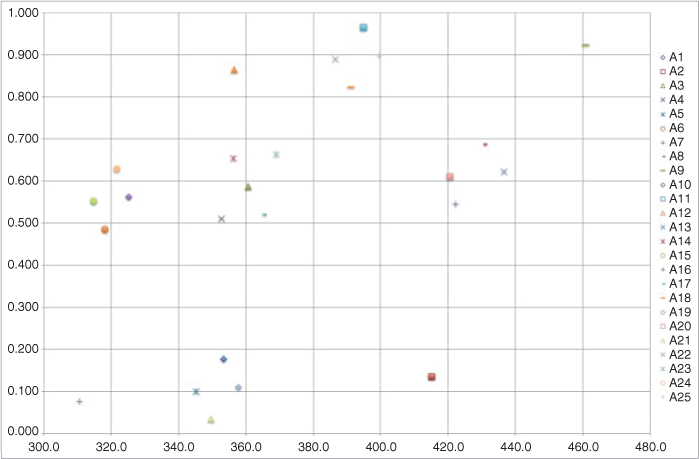
Figure 12.12 Cost versus OMOE for FSSF surface combatant variants
The variants that fall on the Pareto frontier are the ones with the highest OMOE at the lowest cost. These are clustered along a line that traces a path along the upper left edge of the plot. This region is magnified in Figure 12.13 to show the four variants that are nondominated. The four variants range in cost from $314.7 to $394.9 M, and OMOE from 0.629 to 0.966. The selection of the best variant is up to the decision-makers in trading off cost versus effectiveness, as all four solutions are equally optimal in a multiple criteria sense. Affordability considerations (Chapter 4) will be important in this decision. All other variants are dominated by these four, and unless there is significant uncertainty in the variants, these do not need to be considered further in the decision-making process.
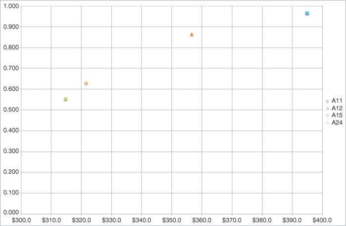
Figure 12.13 Magnified plot region showing only Pareto frontier of nondominated variants for cost versus OMOE for FSSF surface combatants
12.4.4 NATO Surface Combatant Ship Design Tradespace
In order to more thoroughly explore the design space, the factors and response outputs from the DOE are studied using interaction profilers as well as contour profilers. The variables for the design variants are explored by studying their relationship to the outputs used for overall decision-making; in this case, cost and effectiveness, as indicated by OMOE, are used as the basis for decision-making. The resulting Effects plot is shown in Figure 12.14.
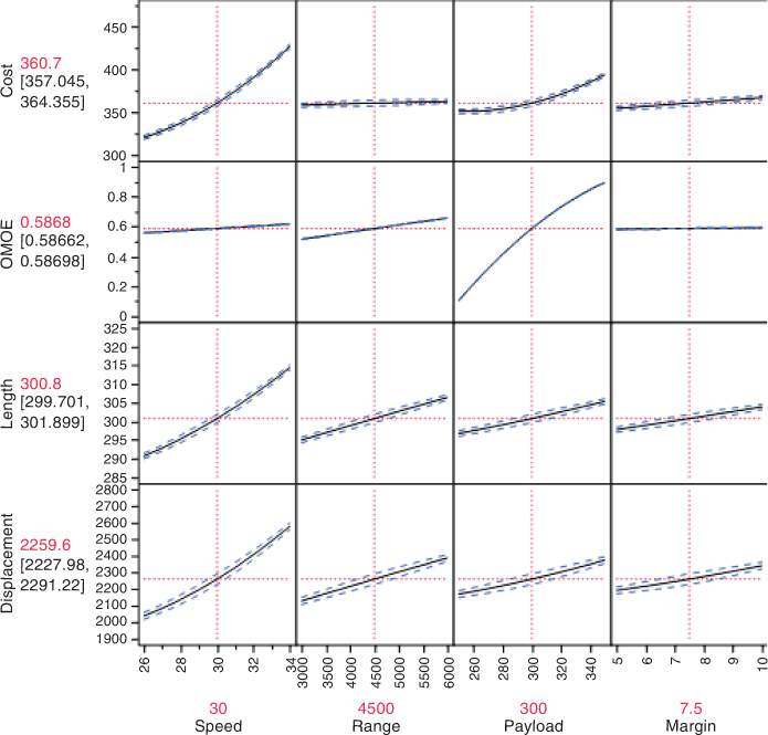
Figure 12.14 Effects plot for NATO FSSF surface combatant ship
By visually inspecting the curves, lines with steep slopes correspond to variables that have substantial impacts on each MOE. The factor that impacts cost the most is speed, while the factor that impacts the OMOE the most is payload. This is confirmed by examining the JMP Effects Pareto Plots, Figures 12.15 and 12.16, with the x-axis as percent effect.
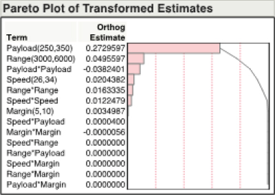
Figure 12.15 OMOE effects Pareto
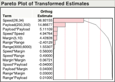
Figure 12.16 Cost effects Pareto
Since payload and speed have the most impact on the design decisions, as indicated by the longest bars in Figures 12.15 and 12.16, respectively, these factors are the primary ones varied to explore the design space. This exploration provides a more detailed look at design possibilities beyond the four Pareto solutions by including variations in the design variables that fall between the data points used for creation of the bounds of the design space.
12.4.5 NATO Surface Combatant Ship Design Trade-Off
To begin with, a series of design space portions have to be viewed on trade-off space plots generated by JMP. The plots can be studied interactively in JMP, but static images are used here to demonstrate a process for investigating the tradespace. The two factors of payload versus speed are plotted with several responses overlaid. For now, the high cost limit is set to $400 M and the low OMOE value is set to 0.83. The resulting feasible design decision space is now shown with a white background in Figure 12.17. The trade-off example is not exhaustive and is used only to show how the process of studying a trade-off space can be accomplished.
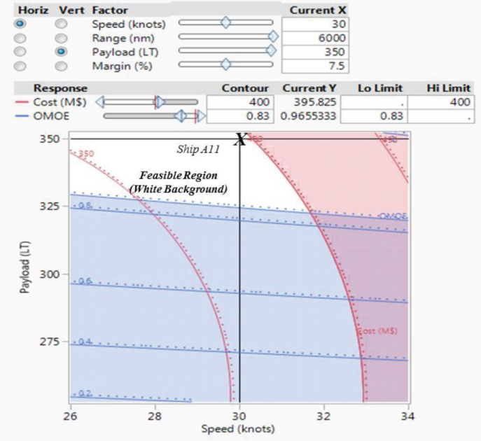
Figure 12.17 Trade-off space of speed versus payload (Ship A11)
The design variant defined by Figure 12.17 is detailed in Table 12.7. Note that Ship A11 is one of the original variants from the DOE table.
Table 12.7 Design Variant
| Ship Variant | Cost | OMOE | Length (ft) | Displacement (Ltons) | Margin (%) | Payload (Ltons) | Speed (knot) | Range (nm) |
| A11 | $395.8 | 0.9655 | 311 | 2491 | 7.5 | 350 | 30 | 6000 |
Ship variant A11 is the best performing alternative with respect to the OMOE that also satisfies the cost constraint of $400 M. However, it may be useful to examine alternative scenarios. As designs mature from concept to preliminary stages, information generated about the design details may make a design impossible to achieve. Unforeseen design changes may also make it impossible to actually create Ship A11. Examination of Figure 12.17 suggests that it may be interesting to examine an alternative ship (termed Ship A11a) that is unable to achieve a total payload of 350 Ltons and can only achieve a payload of 320 Ltons. A visualization of this ship is shown in Figure 12.18; note that it is incapable of satisfying the OMOE constraint of 0.83 and is therefore currently an infeasible system alternative.
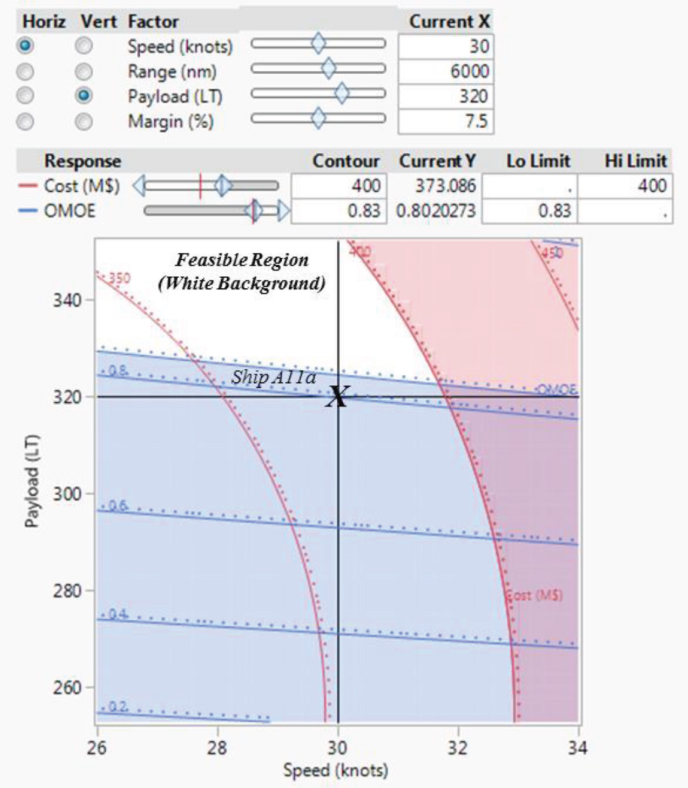
Figure 12.18 Trade-off space of speed versus payload where payload is restricted and the system becomes infeasible (Ship A11a)
The utility of the interactive design space exploration approach is easily demonstrated through presentation of additional design trade-off spaces. For instance, while Figure 12.18 suggests that Ship A11a, which can only achieve a payload of 320 Ltons, is incapable of satisfying the OMOE constraint, examination of an alternative visualization of the trade-off space suggests a potential solution. Figure 12.19 presents a visualization of the same trade-off space but presents the speed and the range (rather than speed and payload, as shown in the previous visualizations).
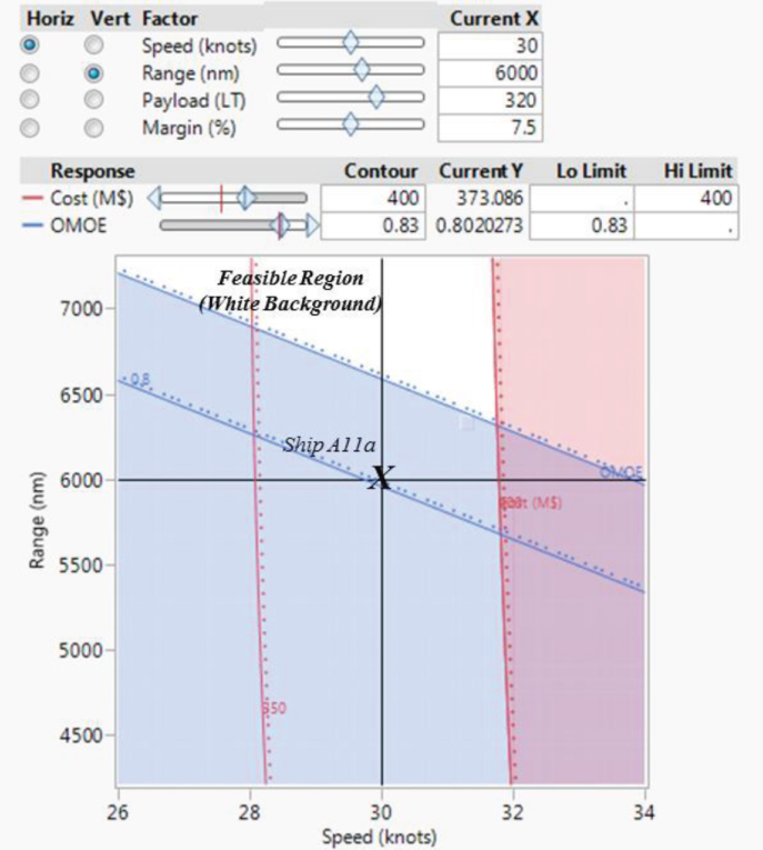
Figure 12.19 Trade-off space of speed versus range (Ship A11a)
Note that Ship A11a is still shown as infeasible, but the alternative visualization suggests that by increasing the range to 6600 nm, the ship (now termed Ship A11b in Figure 12.20) becomes feasible.
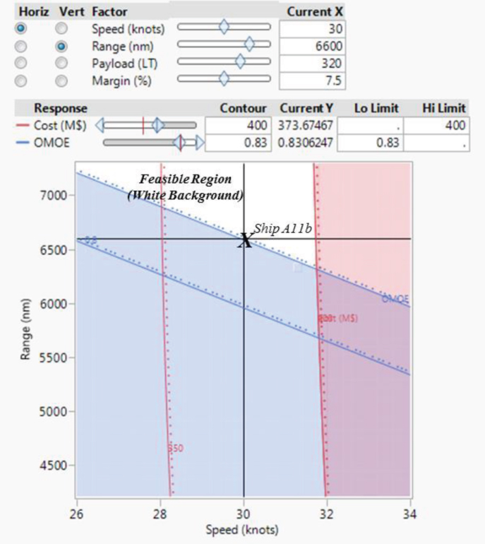
Figure 12.20 Trade-off space of speed versus range (Ship A11b)
The impact of this change can be visualized more clearly by a reexamination of the original trade-off space of speed and payload. Figure 12.21 presents an example of Ship A11b from this perspective. Note that Ship A11b is feasible with respect to both the OMOE and cost despite only having a payload of 320 Ltons (compared to 350 Ltons for the original Ship A11). This is a result of the increase in range from 6000 nm for Ship A11 to 6600 nm for Ship A11b.
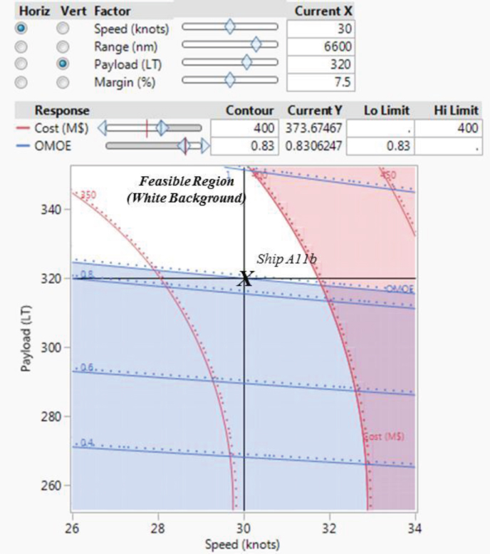
Figure 12.21 Trade-off space of speed versus payload (Ship A11b)
Further study of the feasibility of Ship B with respect to payload versus speed at 5% margin is shown in Figure 12.22. This ship alternative is within the feasible region, indicated with a white background. This example highlighted the utility of the design trade-off space exploration approach for scenarios where constraints are imposed that cause the system to become infeasible. The design trade-off space exploration approach is also useful when requirements are imposed by a stakeholder that may conflict with analysis results. For example, a stakeholder may desire a modification to Ship A11 that increases the speed from 30 to 32 knot while also reducing the payload to 325 Ltons. A visualization of such a scenario is shown in Figure 12.22 (the ship is now termed Ship A11c).
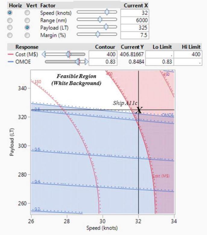
Figure 12.22 Trade-off space of speed versus payload (Ship A11c)
The stakeholder requirement for increased speed, coupled with the decrease in the acceptable payload, has caused the ship to become infeasible with respect to cost. Note that the system can actually become feasible by decreasing the speed to the original value of 30 knot. However, if the stakeholder is unwilling to accept a restricted speed, the design trade-off approach can explore alternative views to define an acceptable system. Figure 12.23 presents a visualization of the trade-off space between the margin and the payload. Note that there is a small feasible region associated with ship configurations with a payload of 325 Ltons and a margin of 5% (reduced from the original value of 7.5%). This ship configuration is plotted as Ship A11d.
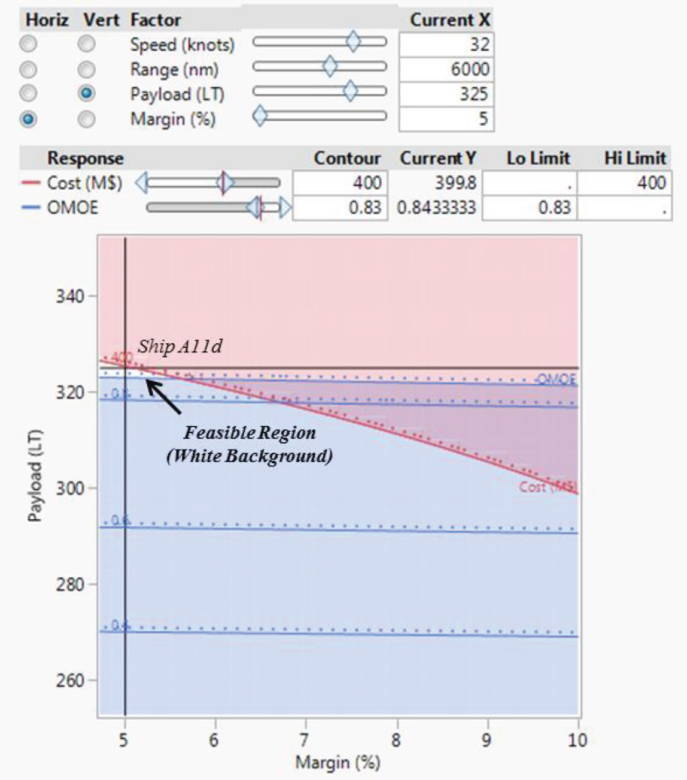
Figure 12.23 Trade-off space of margin and payload (Ship A11d)
Ship A11d is feasible within the cost and OMOE constraints, even though the ship speed is increased to 32 knot and the payload is restricted to 325 Ltons. This highlights the alternative usage of the design trade-off space exploration approach, which allows a stakeholder to examine the impact that system requirements may have on the size of the total number of feasible system configurations as well as the interactions between input factors that must be investigated as a result of each new system requirement.
12.4.6 NATO Surface Combatant Ship Trade-Off Summary
This example shows a design trade-off beginning with consideration of stakeholder needs and requirements and continuing to the development of a DOE trade-off space. Several cost versus Effectiveness optimal solutions are identified from the DOE results. Next, a possible design trade-off is then studied by varying design variable factors and responses to investigate the space for solutions that are interpolated between the DOE points. The resulting designs are summarized in a form that decision-makers can review as a series of variant alternatives that are both feasible and reach the limits of the trade-off since the variables cannot be set to achieve all of the available values simultaneously.
12.5 Key Terms
- Box–Behnken Design: A Box–Behnken design is a three-level experimental design. It has no design points at the vertices of the cube defined by the ranges of the factors. This is sometimes useful when it is desirable to avoid these points due to engineering considerations. The price of this characteristic is the higher uncertainty of prediction near the vertices compared to the central composite design (SAS Institute, 2015a,b).
- Central Composite Designs: A central composite design combines a two-level fractional factorial and two other kinds of points, center points and axial points. The center points are defined such that all the factor values are at the zero (or midrange) value. The axial points are defined such that all but one factor are set at zero (midrange) and that one factor is set at outer (axial) values (SAS Institute, 2015a,b).
- Design of Experiments: A designed experiment is a controlled set of tests designed to model and explore the relationship between factors and one or more responses (SAS Institute, 2015a,b).
- Design Space: A region of interest for a design described by the experimental range of the factor settings chosen for study (SAS Institute, 2015a,b).
- Effects Plots: Graphs that indicate the relationships among the effects in a design.
- Factor Fractional Factorial Design: A design that uses a portion, or fraction, of a full factorial design set of points for the design factors.
- Feasible Region: The area of a design space that contains the points that satisfy constraints and provide solutions.
- p-Value: The calculated probability of finding the observed result when testing a statistical hypothesis.
12.6 Exercises
The following exercises are based on a notional early-stage ship design effort for a small surface combatant, as previously discussed in Section 12.4. This example requires the utilization of JMP to conduct trade-off analysis. Note that the previous example in Section 12.4 utilized a different experimental design and a different dataset, these exercises are focused on the same system but are not related to the data used in Section 12.4.
- 12.1 Upload the following dataset into JMP. Note that the design is a central composite design generated using JMP. The three responses (cost, OMOE, and displacement) are functions of the four factors (speed, range, payload, and margin). Use the Analyze → Fit Model functionality in JMP to develop prediction formulas for each of the responses. When prompted to Construct Model Effects, include all two-way interactions (using the Factorial to Degree functionality) as well as all quadratic effects (using the Polynomial to Degree functionality). Conduct Least Squares Regression and save the prediction formula (Save Columns → Save Prediction Formula) for each of the responses.
- 12.2 Open a Contour Profiler (Graph → Contour Profiler) using each of the prediction formulas developed in Problem 1. Impose constraints for each of the responses. Impose a high limit on cost of $1750 M, a low limit on OMOE of 0.50, and a high limit on displacement of 4750 Ltons. Describe the feasible space.
- 12.3 Based on your response to Problem 2, explore alternate two-dimensional projections (projections other than speed and range) and suggest at least two potential feasible ship configurations without altering any of the constraints imposed on the responses.
Pattern Factors Responses Speed (knot) Range (nm) Payload (Ltons) Margin (%) Cost (M$) OMOE Displacement (Ltons) −−−− 26 3000 250 5 398.81185 0.0104 3484.287 −−−+ 26 3000 250 10 675.443203 0.3020 3848.332 −−+− 26 3000 350 5 656.090758 0.5811 3707.986 −−++ 26 3000 350 10 911.019546 0.8458 4028.422 −+−− 26 6000 250 5 1828.8852 0.0338 3976.728 −+−+ 26 6000 250 10 2295.84548 0.3125 4330.991 −++− 26 6000 350 5 2169.71101 0.6055 4206.921 −+++ 26 6000 350 10 2642.01684 0.9904 4541.402 +−−− 34 3000 250 5 950.393424 0.0245 5444.087 +−−+ 34 3000 250 10 1210.58148 0.3369 5741.125 +−+− 34 3000 350 5 1268.01422 0.6970 5505.467 +−++ 34 3000 350 10 1532.41456 0.9007 5961.524 ++−− 34 6000 250 5 2474.35812 0.0498 5998.325 ++−+ 34 6000 250 10 2920.50349 0.3519 6204.49 +++− 34 6000 350 5 2725.02865 0.7573 6132.663 ++++ 34 6000 350 10 3185.3991 0.9697 6477.513 a000 26 4500 300 7.5 1379.07059 0.4224 4063.652 A000 34 4500 300 7.5 1978.00227 0.4873 6052.191 0a00 30 3000 300 7.5 969.966418 0.4399 4727.896 0A00 30 6000 300 7.5 2466.02425 0.4951 5212.494 00a0 30 4500 250 7.5 1517.93628 0.1128 4759.32 00A0 30 4500 350 7.5 1750.40849 0.7623 5032.142 000a 30 4500 300 5 1490.98832 0.2887 4870.674 000A 30 4500 300 10 1797.51409 0.6535 5151.25 0 30 4500 300 7.5 1629.584 0.4304 4882.302 0 30 4500 300 7.5 1586.39436 0.5131 4934.937 - 12.4 After selecting a feasible ship configuration (from Problem 3), reset the axes such that the speed is shown on the x-axis and the range is shown on the y-axis. Compare the feasible and infeasible spaces shown to the original feasible space identified in Problem 2. The constraints have not changed and the two-dimensional projection has not changed, why has the shape of the feasible region changed?
- 12.5 Provided that there is a feasible region shown in the answer to Problem 4, select a design point in the feasible region (if there is not, alter the payload and/or margin to create a feasible region). Next, change the y-axis from range to payload. Is the selected design point still feasible? Change the y-axis to Margin, is the selected design point still feasible? Discuss why changing the axes does not alter the feasibility of the selected design point.
- 12.6 Reset each of the factor values to their initial levels (30 knot speed, 4500 nm range, 300 Ltons payload, and 7.5% margin). Increase the OMOE constraint to 0.80. Identify the changes necessary to define a feasible set of ship configurations. Is it possible to select a ship configuration with a speed of 30 knot? If not, what constraint must be relaxed to enable the selection of such a ship? Is it possible to select a ship with a maximum range of 5000 nm? If not, what constraint must be relaxed to enable the selection of such a ship?
- 12.7 The previous question suggested that it may be desirable to relax constraints to enable the selection of ships with higher speed or a higher range. However, this example utilizes three responses that address the cost, effectiveness, and physics (through the displacement of each ship). Discuss how such a tool can be used to highlight potentially unnecessary increases to factors such as speed and range.
References
- Katsoufis, G. (2006) A decision making framework for cruise ship design, Master thesis, MIT.
- NATO (2004) NATO/PfP Working Paper on Small Ship Design, NATO Naval GROUP 6 SPECIALIST TEAM ON SMALL SHIP DESIGN.
- SAS Institute Inc (2015a) JMP® 12 Design of Experiments Guide, SAS Institute Inc., Cary, NC, ISBN 978-1-62959-443-9.
- SAS Institute Inc (2015b) Using JMP® 12, SAS Institute Inc., Cary, NC, ISBN 978-1-62959-479-8.