
13
Harmonics in Power Systems
Ideally the currents flowing throughout the power system should be sinusoidal, since the voltages exciting them are sinusoidal, or nearly so. However, when a customer’s load contains non‐linear (or distorting) elements then non‐linear currents will occur as a result. Such currents can be resolved into a component at the system frequency, henceforth referred to as the fundamental frequency (f1), and harmonic components occurring at integral multiples of the fundamental (nf1). Therefore we might expect 2nd, 3rd, 4th and 5th harmonic currents, for example, to appear as a result of distorting loads connected to the network; however, we will see that under most conditions even harmonics are generally absent.
Harmonics are not new; as long ago as 1916 the third harmonic, caused by the saturation of machines and power transformers, was noticeable. Improvements in transformer design reduced this problem substantially until the 1930s when the introduction of large rectifier equipment for rail transport again introduced significant harmonics into the power system. Interestingly, the main problem presented by harmonics was interference with the open wire telephony circuits of the day.
Prior to 1960 one of the main sources of harmonic distortion was television receivers with power supplied from a half wave rectifier. As a result each receiver introduced a small DC current into the LV network, as well as even and odd harmonics. The DC currents in the LV network approximately cancelled due to the fact that the AC connector could be reversed, but any residual current created a DC flux in distribution transformers, increasing their magnetising losses slightly. During the period 1960–75 the availability of thyristors led to the introduction of phase‐controlled dimmers for domestic and industrial lighting and heating applications. These produced considerable harmonic distortion, as well as high frequency radio emissions, and led to the publication of the first standards restricting harmonics in power systems.
The 1980s and early 1990s saw a rapid expansion in the use of on line switch mode power supplies in television receivers, personal computers and numerous other consumer appliances. These employed single‐phase full wave rectifiers and capacitive filters which consumed short duration, high amplitude current pulses, close to the peak of the AC cycle. This resulted in a substantial flattening of the peak of the AC waveform, as well as the generation of many low‐order harmonics, particularly the third, fifth and seventh. This period saw the development of European standards on consumer products, and by 1995 IEC 61000‐3‐2 defined requirements and harmonic current limits for four classes of consumer equipment, Classes A–D.
Today, in addition to a vast array of consumer electronics, there are also many large non‐linear devices connected to the power system. With the advent of high current thyristors and insulated gate bipolar junction transistors (IGBJTs), AC to AC and AC to DC converter circuits frequently appear in industrial loads. Since this equipment is inherently non‐linear, the current it consumes is often rich in harmonics.
The presence of harmonics in the power system leads to many adverse effects, including increased losses in transmission lines, transformers and rotating machines, in addition to the possible mal‐operation of some items of customer equipment. We will show that the presence of harmonic currents requires that the power factor definition be amended to include their effects, and that harmonic currents always act to reduce the total power factor of a load.
Harmonics generated by one customer may interfere with the load of another, and to avoid this, the background level of individual harmonics in the system must be carefully managed. This task falls broadly into two areas. Firstly, it is the responsibility of customers to ensure that any harmonic distortion their load creates does not exceed the emission limit defined in the relevant standard or in the supply agreement with the network service provider. This may require selection of equipment designed to avoid excessive harmonic generation, or the installation of harmonic filters to ameliorate their effects. The connection agreement either places limits on the customer’s contribution to the harmonic voltage distortion or to the harmonic currents that can be injected into the network at the customer’s connection point, or alternatively at the point of common coupling between the customer’s load and other loads on the network. (A limit on the harmonic currents that may be injected is relatively easy to enforce, since the harmonic current spectrum can be measured with an energy meter having power quality capabilities. On the other hand, determining the component of harmonic voltage distortion introduced by a particular customer is not so straightforward, unless the harmonic impedances are known at the point of common coupling.)
Secondly, the network service provider also has a responsibility to ensure that the level of harmonic distortion allocated to each new customer does not result in an overall harmonic level sufficient to cause disturbances to any customer equipment. This usually requires an investigation of a customer’s proposed load prior to connection, in addition to a knowledge of the background level of harmonic distortion pre‐existing in the network. (It is much easier to determine the background voltage distortion levels prior to connection of the proposed load than post connection.)
Harmonic Propagation
Harmonic sources can usually be modelled by a harmonic current source connected in parallel with a distorting load. As a result, harmonic currents are shared between those linear components of the load and the upstream network where they generate small harmonic voltages across the local network impedance. This produces a degree of harmonic voltage distortion which is propagated throughout the network. Thus the effect of one customer’s distorting load is frequently felt by others.
Where harmonic disturbances must be suppressed, it is common to install harmonic filters within or close to the offending load. Large variable speed drives, for example, are often designed to minimise the export of harmonic currents to the upstream network. Alternatively, harmonic filters can be installed in parallel with a load. These are circuits designed to provide an alternative low impedance path for selected harmonics, which may then flow harmlessly to ground rather than into the local network. In this way, harmonic voltage distortion can be minimised, together with the harmonic current the load injects into the network.
13.1 Measures of Harmonic Distortion
There are several simple numerical measures of the harmonic content of either a voltage or a current. We will consider the total harmonic distortion (THD), the total demand distortion (TDD) and the crest factor (CF). However, we initially consider the RMS current arising from a fundamental current together with an assortment of its harmonics, which can be expressed in the form:

A similar result applies for voltage, thus:

Where Ih and Vh are the current and voltage magnitudes of the harmonic h respectively and hmax is the maximum harmonic order present.
The total harmonic current distortion (THDi) is the ratio of the RMS harmonic current present to the fundamental current, expressed as a percentage:

(Note that the RMS summation in Equation (13.3) excludes the fundamental component.)
Similarly the total harmonic voltage distortion (THDv):

Handheld instruments are capable of determining the THD of voltage and current waveforms, and in some cases they are also able to resolve the levels of the individual harmonics present.
It is possible for a load to exhibit quite high THDi at times when the fundamental current demand is low, without imposing an unacceptable burden on the network, and thus the THDi can provide a slightly misleading estimate of a load’s actual harmonic content. The total demand distortion (TDD) is a way of quantifying the harmonic content in terms of the fundamental current, corresponding to the maximum VA demand. The TDD is the ratio of the (worst case) RMS harmonic current to the fundamental component at maximum demand. The expression for TDD is therefore similar to that for THDi, except that the RMS harmonic current is referenced to the maximum demand load current IL, rather than the fundamental current recorded at the time of the measurement, I1. The TDD will therefore be lower that the THDi and is used to define the harmonic current limits in IEEE Std 519‐2014, Recommended Practice and Requirements for Harmonic Control in Electric Power Systems.

As well as THD and TDD, the crest factor of a waveform (usually a current) is also used as a measure of its harmonic content. This is defined as follows:

The crest factor provides a measure of the ‘peakiness’ of a waveform. So, for a current or voltage without significant harmonic content, the crest factor will be close to ![]() . Crest factors higher than this correspond to peaky waveforms, while values less than
. Crest factors higher than this correspond to peaky waveforms, while values less than ![]() relate to flat topped waveforms, both of which imply that harmonics are present. However, a heavy harmonic content is generally characterised by large crest factors. Such loads impose a severe burden on the source of power supplying them, since unless the peak current can be delivered, the supply voltage at the load will become distorted. Well‐designed loads will therefore have crest factors approaching
relate to flat topped waveforms, both of which imply that harmonics are present. However, a heavy harmonic content is generally characterised by large crest factors. Such loads impose a severe burden on the source of power supplying them, since unless the peak current can be delivered, the supply voltage at the load will become distorted. Well‐designed loads will therefore have crest factors approaching ![]() .
.
While all these indices provide a useful quantitative measure of harmonic distortion, they provide no information as to which of the harmonic(s) present have the largest amplitude and therefore should be targeted in the first instance. We will see that harmonic components roughly diminish as 1/h (or sometimes as 1/h2), and therefore it is frequently the lower‐order harmonics that are most problematic.
13.2 Resolving a Non‐linear Current or Voltage into its Harmonic Components (Fourier Series)
Sinusoidal waveforms, be they voltage or current, have the unique property that they only contain energy at one frequency. It was shown in 1822 by Joseph Fourier, in his solution to the heat equation, that any other periodic wave shape can be resolved into a series of sinusoidal components at different frequencies; specifically the fundamental frequency and a series of harmonics. The fundamental frequency is the reciprocal of the period T of the waveform and harmonics are integer multiples of this frequency.
In the steady state analysis of AC networks, voltages and currents are represented by periodic functions. A function f(t) is said to be periodic with period T, if for any t we can write:
Any periodic function may be decomposed into a sum of its Fourier components, consisting of a DC term (or average value), a component at the fundamental frequency, plus a series of harmonic components, represented by sine and cosine functions at integer multiples of the fundamental frequency. The Fourier series of a periodic current i(t) can be expressed as follows:

where ![]() is the angular frequency of the fundamental component and iDC is the average value of the waveform i(t), i.e.
is the angular frequency of the fundamental component and iDC is the average value of the waveform i(t), i.e.

The weightings ak and bk are known as the Fourier coefficients, and are given by:

Thus any function (except for purely sinusoidal functions, where ak and ![]() for all k ≠ 1), can be expressed as a DC term (should one exist), a component at the fundamental frequency, plus a sum of harmonic components.
for all k ≠ 1), can be expressed as a DC term (should one exist), a component at the fundamental frequency, plus a sum of harmonic components.
By way of example, consider the current waveform shown in Figure 13.1. This is typical of the current drawn by a power supply consisting of a full wave bridge rectifier with a simple capacitive filter, as found in many personal computers and other consumer equipment. The waveform consists of a current pulse near the crest of the voltage; its harmonic spectrum shows that it contains no even harmonics, and the magnitudes of the third and fifth harmonics are comparable to that of the fundamental. As a result, the total harmonic current distortion of this waveform is in excess of 100% and its crest factor is about 3.5. In recent years, manufacturers of computing equipment have begun to move away from this type of power source, constructing instead power factor corrected supplies. These present an almost resistive load, and do not consume significant harmonic currents.
Figure 13.1 (a) Personal computer current and voltage waveforms (b) Current harmonic spectrum.
13.2.1 Fourier Simplifications Due to Waveform Symmetry
Not all waveforms contain both sine and cosine terms. For example, if a waveform has odd symmetry there are no cosine terms. Odd symmetry exists if ![]() , after any DC term has been removed, therefore it can be shown that
, after any DC term has been removed, therefore it can be shown that ![]() . Similarly the sine terms are absent if the signal has even symmetry whereby
. Similarly the sine terms are absent if the signal has even symmetry whereby ![]() , after any DC terms have been removed, thus
, after any DC terms have been removed, thus ![]() .
.
Of more importance from the point of view of power system harmonics is the concept of half wave symmetry, which exists if the positive and negative halves of a waveform are identical in shape but opposite in sign, i.e. ![]() . When a waveform has half wave symmetry it contains no even harmonics. Half wave symmetry is common in power systems and thus most current or voltage waveforms contain only odd harmonics. The current waveform in Figure 13.1 is a case in point. Note that the presence of a DC term precludes half wave symmetry. As a result of half wave symmetry, the Fourier coefficients can be expressed in the form:
. When a waveform has half wave symmetry it contains no even harmonics. Half wave symmetry is common in power systems and thus most current or voltage waveforms contain only odd harmonics. The current waveform in Figure 13.1 is a case in point. Note that the presence of a DC term precludes half wave symmetry. As a result of half wave symmetry, the Fourier coefficients can be expressed in the form:

Examples: Consider the square waveform shown in Figure 13.2. By inspection it has both odd symmetry and half wave symmetry, and thus it contains no cosine terms and no even harmonics.

Figure 13.2 Square waveform.
In this case, the only non‐zero Fourier coefficients are bk when k is odd. Thus:

This result is interesting, since the odd harmonics present decrease as 1/k, thus higher‐order harmonics tend to have smaller amplitudes. This fact is significant in reducing the impact of large non‐linear loads on power systems, as will be shown later.
Consider the triangular waveform in Figure 13.3. Here even symmetry and half wave symmetry exist, so the triangular waveform will have no sine terms and no even harmonics. Accordingly ak is given by:


Figure 13.3 Triangular waveform.
And the harmonics decrease as 1/k2.
Finally, consider the half wave rectified current waveform in Figure 13.4. This has a DC term and therefore has no half wave symmetry, although it does have even symmetry, thus ![]() .
.

Figure 13.4 Half wave rectified current.
So:

In this case, there are no odd harmonics, and this waveform contains harmonic components whose amplitude decrease approximately as 1/k2. The DC component of this current is given by:

13.2.2 Transformer Inrush Current (Second Harmonic Restraint)
Since half wave symmetry occurs frequently, odd harmonics generally occur much more often than even ones. There is one particular instance, however, where a transient DC term occurs and with it the brief existence of even harmonics. The situation in question relates to the inrush currents that flow when a transformer is energised. Depending on the instant of switching, the magnetising current may take on values very much higher than normal. This phenomenon was discussed in Section 7.5.4, and Figure 7.18 illustrates typical magnetising currents that arise immediately after switch on. Until the B–H loop re‐centres itself on the origin, the magnetising current possesses a DC component in addition to even harmonics.
This fact is used to advantage by protection engineers who must protect transformers from faults at switch‐on, as well as during normal operation. The large inrush current can cause false trips in transformer differential protection relays (which compare primary and secondary currents on an instantaneous basis). Since the magnetising current is consumed within the transformer, the large inrush appears as an internal fault to a differential relay, which therefore must be restrained for a short period following switch‐on.
Inrush current can be distinguished from fault current by detecting the presence of even harmonics, notably the second harmonic, since it is generally the largest. In this instance, transformer protection relays are usually restrained from operating for a period, so long as there is a sufficiently large second harmonic component present. This restraint may mean that trips are inhibited entirely until the steady state has been achieved (which can take tens of seconds) or alternatively, a group of higher trip settings are enabled instead, so that should a fault also occur at switch on, the transformer will still be protected. Once the steady state has been reached and the even harmonics have disappeared, the normal protection settings are restored.
13.3 Harmonic Phase Sequences
Since large non‐linear industrial loads such as variable speed drives are generally well balanced, so are the harmonics that they create. In other words currents or voltages of a particular harmonic tend to exist as balanced three‐phase systems in their own right. This enables them to assume either positive, negative or zero‐sequence characteristics.
Consider the case of a balanced three‐phase system of currents from a distorting load, including harmonics. The fundamental phase currents may be expressed as:

In general, the hth order harmonic takes the form:

where Fh is a harmonic scaling factor, and depends on the shape of the current waveform in question. Generally Fh will diminish as h increases, possibly as 1/h or 1/h2.
Of significance here is the fact that not only is the frequency of the fundamental scaled by the factor h, but also its phase as well. These equations demonstrate that when the fundamental currents are balanced then so are their harmonics. However, this does not necessarily mean that the phase sequence of these harmonics is the same as that of the fundamental. Consider, for example, the case of the third harmonic:

Since the third harmonic phase shifts are three times as large as those of the fundamental, the resulting third harmonic currents are co‐phasal. In other words, the third harmonic is a zero‐sequence harmonic. This property is also true of any harmonic that is a multiple of three, i.e. the 3rd, 6th, 9th etc. These harmonics are often called triplen harmonics.
Non‐triplen harmonics may have either a positive or a negative phase sequence. In the case of the 5th harmonic we find:

Comparing these equations with those of the fundamental, we see that the B and C phasors have swapped positions, and therefore the phase sequence of the 5th harmonic is ACB; it is therefore a negative sequence harmonic. In contrast the 7th is a positive sequence harmonic, as shown below.

Harmonic phase sequences are summarised in Table 13.1.
Table 13.1 Harmonic phase sequences.
| Positive sequence harmonics (+) | Negative sequence harmonics (−) | Zero‐sequence harmonics |
| 1st | 2nd | 3rd |
| 4th | 5th | 6th |
| 7th | 8th | 9th |
| 10th | 11th | 12th |
| 13th | 14th | 15th |
13.3.1 Voltage Harmonic Distortion
Even harmonics are rare in power systems, so the odd harmonics tend to be the most troublesome, and since these generally diminish with the harmonic number, it is the first few odd harmonics (3rd, 5th, 7th, 11th and 13th) that can be problematic. Longer duration harmonic currents (existing for 10 minutes or more), cause additional losses in rotating machines, transformers and transmission lines, while in the very short term (less than 3 seconds), elevated levels of harmonic voltage distortion may lead to the mal‐operation of some items of customer equipment.
In order to avoid the propagation of harmonic currents throughout the entire network, harmonic standards require that network operators maintain relatively low levels of harmonic voltage distortion, particularly at transmission potentials. Because most distorting loads exist in the LV network (and to a lesser extent in the MV), it is to be expected that voltage distortion will be highest at LV potentials, becoming progressively less so at MV and HV. Some typical harmonic planning levels used by network owners at various network voltages are shown in Table 13.2. These can be considered a quality objective to be achieved in a particular locality where various distorting loads are connected. They are used in the establishment of the harmonic emission limits assigned to individual customers, taking into account all distorting loads connected to the local network, with the aim of sharing the capacity of the network to absorb harmonic currents between all customers.
Table 13.2 Typical harmonic planning levels for low‐order, non‐triplen harmonics.
| Typical voltage distortion planning limits (% of Fundamental) | |||||
| Harmonic | EHV | 33–69 kV | 11–22 kV | 6.6 kV | 400 V |
| 5th | 2.00 | 3.1 | 5.1 | 5.3 | 5.5 |
| 7th | 2.00 | 2.7 | 4.2 | 4.3 | 4.5 |
| 11th | 1.5 | 1.9 | 3.0 | 3.1 | 3.3 |
| 13th | 1.5 | 1.8 | 2.5 | 2.6 | 2.8 |
Table 13.2 shows that harmonic planning levels are considerably reduced at HV potentials as compared to those at MV and LV. In addition, as the harmonic number increases, the planning level reduces. This is largely due to the natural tendency for the harmonic amplitude to reduce with increasing harmonic number. More will be said about planning levels and emission limits in Section 13.8.
Finally, in the unusual case where the distorting load is particularly unbalanced, then so will be the harmonics it creates. In this situation, all harmonics behave in a similar fashion to unbalanced fundamental currents, each having positive, negative and zero‐sequence components.
13.4 Triplen Harmonic Currents
Because of their zero‐sequence characteristics triplen harmonics can be the source of localised overheating problems, particularly in LV neutral conductors where the residual current flows towards the star point of the supply transformer. Since network owners attempt to balance LV loads evenly across all three phases, the neutral conductor is generally not expected to carry a significant current. However, this situation can change dramatically in the presence of triplen harmonic currents (notably the third), since these accumulate in the neutral and may become sufficiently large to overload this conductor.
Consider the case of a distorting LV load including a ‘modest’ 40% third harmonic component, in addition to the fundamental. The resulting RMS phase current will be:
This current is little different from that which might be expected to flow in each phase in the absence of harmonics, but the amplitude of the neutral current will be an unexpected ![]() . This can overload the neutral conductor which may be of a smaller size than the associated phase conductors. One method often used in larger LV networks to reduce this effect is to install a grounded zigzag transformer on the LV bus, close to the distorting load. Operating in a similar way to an earthing transformer, this arrangement provides a low zero‐sequence ground impedance, diverting much of the 3rd harmonic current away from the supply transformer and out of the neutral conductor(s), in addition to reducing the transformer’s triplen harmonic loss. To assist this, a small inductance is often inserted in the neutral connection of the distribution transformer, to increase its zero‐sequence impedance and therefore further reduce the triplen harmonic current flowing.
. This can overload the neutral conductor which may be of a smaller size than the associated phase conductors. One method often used in larger LV networks to reduce this effect is to install a grounded zigzag transformer on the LV bus, close to the distorting load. Operating in a similar way to an earthing transformer, this arrangement provides a low zero‐sequence ground impedance, diverting much of the 3rd harmonic current away from the supply transformer and out of the neutral conductor(s), in addition to reducing the transformer’s triplen harmonic loss. To assist this, a small inductance is often inserted in the neutral connection of the distribution transformer, to increase its zero‐sequence impedance and therefore further reduce the triplen harmonic current flowing.
An alternative way of avoiding triplen neutral currents is to operate a star connected load without a neutral connection, although clearly this method is unsuitable for LV loads. Without a neutral connection, triplen currents cannot flow and, as a result, a triplen oscillation occurs at the star point, in a similar fashion to that described in Section 7.5.1. This method is frequently used in voltage support capacitor banks and harmonic filters, where it is usually desirable to avoid triplen currents.
13.5 Harmonic Losses in Transformers
Winding temperatures in all transformers are exacerbated by the presence of harmonic currents, particularly as the harmonic number increases, due to the effects of the additional eddy current losses occurring within the conductors themselves. These losses arise as a result of the electromagnetic field surrounding a current carrying conductor, produced by the current itself. When the associated flux passes through the face of a conductor, a small potential is generated which causes eddy currents to circulate around the conductor periphery, in much the same way as eddy currents occur within magnetic laminations. The associated losses increase the temperature of the winding and any other metallic components in which they occur. They are proportional to the square of the electromagnetic field strength (and thus the square of the current producing it), as well as to the square of the frequency of the field.
Eddy current losses are frequently concentrated towards the ends of the winding closest to the core (usually the LV winding) since the flux there has a tendency to fringe towards the core, passing through the face of conductors as it does so. Because these losses vary as the square of both the current and frequency, high‐order harmonics can have a disproportionate influence, despite their having generally lower amplitudes.
Some small distribution transformers are built without oil immersion cooling. This saves considerably on size, weight and expense, but these transformers are totally reliant on natural airflow for their cooling. They are known as dry transformers, and as shown in Figure 7.1b, their windings are cast in epoxy resin. Because they are not flooded with oil, the heat generated must be dissipated by conduction through the windings themselves and convection and radiation from their surfaces. This can lead to high hot spot temperatures occurring, particularly in the presence of a harmonic rich load. If the hot spot temperature exceeds the insulation’s limiting temperature, it will become degraded, reducing the expected life of the transformer.
The cooling of all transformers becomes considerably more difficult in the presence of harmonics, to the extent that harmonic rich loads may demand the de‐rating of the transformer concerned.
13.5.1 Harmonic Loss Factor
The IEEE standard C57.110 Recommended Practice for Establishing Liquid Filled and Dry Type Power and Distribution Transformer Capability when Supplying Non‐Sinusoidal Load Currents, considers the effect of the harmonic content of the load current in establishing the effective capacity of a transformer when supplying non‐sinusoidal load currents. A transformer’s load losses (those associated with its load current as opposed to magnetising losses) can be expressed, in terms of the symbolism of C57.110, as:
where PLL is the total load loss (watts), I2R is the resistive portion of the load loss, and I is the RMS load current flowing, PEC is the winding eddy current loss and POSL is the other stray losses.
An allowance is made for the eddy current loss (PEC) occurring at the fundamental frequency in the design of a transformer. However, this loss increases substantially in the presence of harmonic load currents and so the rated capacity of the transformer must often be reduced when a significant harmonic content is present.
The other stray losses include eddy current losses in the tank walls, clamping structures and internal busbars etc., and since these also increase the cooling load on liquid‐filled transformers, they must also be included in the overall transformer loss. Dry transformers on the other hand, are not so restricted, since losses in clamping structures do not generally affect the temperature of the windings, as both reject heat independently into the atmosphere.
Since the eddy current loss is proportional to the square of the harmonic frequency, the total eddy current loss, including contributions at both the fundamental and harmonic frequencies, is given by:

where ![]() is the measured eddy current loss at the fundamental frequency,
is the measured eddy current loss at the fundamental frequency, ![]() is the rated eddy current loss at the fundamental frequency, Ih is the RMS current of order h, I is the measured RMS transformer secondary current
is the rated eddy current loss at the fundamental frequency, Ih is the RMS current of order h, I is the measured RMS transformer secondary current  , IR is the rated fundamental current of the transformer and Ih(pu) is the per‐unit harmonic current (relative to the rated fundamental current).
IEEE C57.110 defines the harmonic loss factor (FHL) for a transformer as:

where I1 is the RMS fundamental load current.
F HL quantifies the increase in the eddy current loss occurring in the presence of harmonic currents. As suggested by Equation (13.7), it can be calculated from per‐unit measurements of the harmonics present as assessed using a handheld harmonic analyser. FHL can therefore be readily determined for any particular load spectrum. It is used in determining by how much a transformer must be de‐rated when supplying a particular spectrum of harmonic currents, as shown in the following example for a dry type transformer.
13.5.2 Harmonic Capacity Constraints in Dry‐Type Transformers
Consider the de‐rating necessary for a dry transformer when supplying a harmonic rich load. Since the stray loss component POSL does not substantially affect the winding temperature of a dry transformer, it can be ignored. Equation (13.6) can then be written in per‐unit form, where the rated resistive loss IR2R is taken as the base:
However, since in the presence of harmonics the measured load current may exceed the rated current, each term is scaled according to the square of the measured per‐unit load current I(pu)2 to yield the actual per‐unit load loss PLLact(pu), dissipated by the transformer.
When the transformer carries its rated fundamental current the measured eddy current loss ![]() , becomes equal to the rated eddy current loss
, becomes equal to the rated eddy current loss ![]() , thus we may write:
, thus we may write:
If the transformer is not to be overheated by the additional eddy current losses, then the actual load loss PLLact(pu) must remain less than or equal to the rated load loss, ![]() applicable to the transformer, i.e.:
applicable to the transformer, i.e.:
We may rearrange Equation (13.9) to obtain the maximum per‐unit load current that can be permitted to flow in the transformer in the presence of harmonics, subject to preserving its rated load loss, thus:
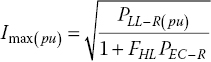
Example: Consider a transformer in which the load current has the harmonic spectrum shown in Table 13.3. Assume that the magnitude of the rated eddy current loss ![]() occurring at the fundamental frequency is 15% of the rated I2R load loss. Therefore the total rated load loss
occurring at the fundamental frequency is 15% of the rated I2R load loss. Therefore the total rated load loss ![]() is 1.15 pu.
is 1.15 pu.
Table 13.3 Harmonic Spectrum.
| h | 1 | 5 | 7 | 11 | 13 | 17 | 19 |
| Ih/I1 | 1.00 | 0.24 | 0.12 | 0.048 | 0.029 | 0.015 | 0.009 |
From the harmonic spectrum the RMS load current I can be calculated, since  . Next, the harmonic loss factor FHL can be evaluated, as shown in Table 13.4.
Table 13.4 Harmonic calculations.
| h | (Ih/I1) | (Ih/I1)2 h2 |
| 1 | 1.00 | 1.00 |
| 5 | 0.24 | 1.44 |
| 7 | 0.12 | 0.705 |
| 11 | 0.048 | 0.279 |
| 13 | 0.029 | 0.142 |
| 17 | 0.015 | 0.065 |
| 19 | 0.009 | 0.029 |
| Σ = 3.66 | ||
Thus:

We can now apply Equation (13.10) to obtain the per‐unit maximum non‐sinusoidal load current which the transformer can safely support:

Therefore as a result of the harmonic content in its load, this transformer must be de‐rated by 13%. A similar approach is used in evaluating the maximum load current for oil‐filled transformers, except that in this case the other stray losses (POSL) must also be taken into account, since they also contribute to the transformer top oil temperature and therefore to the winding temperature as well. Examples of such calculations are provided in IEEE C57.110.
13.5.3 K‐Factors
The concept of a K‐factor was introduced by the Underwriter’s Laboratory in the USA in the early 1990s. This index is an indication of a transformer’s ability to supply a harmonic rich load while operating within the temperature limitations of its insulation. The K‐factor is defined as:

where Ih is the RMS value of harmonic current h and IR is the rated transformer current.
The K‐factor is clearly similar to the harmonic loss factor, except that it is based on the rated transformer current IR rather that the actual load current flowing I. As a result, the K‐factor for a given load varies inversely with the size of the transformer.
Manufacturers build K‐rated transformers capable of supplying load currents of a particular K‐factor. These oversized transformers require no further de‐rating, provided the K‐factor of the connected load is less than or equal to that for which the transformer has been built. Designers take the following steps to reduce the effects of eddy current losses in a K‐rated transformer:
- Design the core to operate at a lower flux density than might normally be chosen, so as to reduce the magnetising losses.
- Provide oversized windings comprising several parallel connected conductors to mitigate the increased resistance due to the skin effect at harmonic frequencies. This technique allows harmonic currents to be carried by several conductors. By so doing, the total resistance at each harmonic is reduced, since a greater portion of each conductor is used to carry current, reducing the total harmonic loss in the winding.
- Provide increased clearances between the core and other metallic components such as the windings and the tank. The use of non‐magnetic materials (where possible) and the avoidance of closed circulating current paths within clamping structures, as well as the use of magnetic shielding materials to avoid inducing eddy currents within metallic components, all contribute to a reduction in these losses.
- Provide an oversized neutral conductor to avoid the excessive heating effects of triplen harmonics.
Table 13.5 shows some typical transformer K‐ratings and their likely applications.
Table 13.5 K‐factor transformer ratings and applications.
| K‐factor rating | Harmonic content | Likely application |
| 1 | Nil | Sinusoidal loads, resistive heating, incandescent lighting, motors (without VSDs) |
| 4 | 16% 3rd, 10% 5th 7% 7th, 5.5% 9th | Welders, induction heaters, high intensity discharge lighting, fluorescent lighting |
| 9 | 150% of the harmonic loading of a K4 transformer | Healthcare facilities, schools, office buildings |
| 13 | 200% of the harmonic loading of a K4 transformer | UPS & VSD systems, healthcare facilities, schools |
| 20 | Very large | Critical care areas in hospitals, operating facilities, data processing equipment, computer installations |
13.6 Power Factor in the Presence of Harmonics
Just as harmonics increase the losses within individual transformers, they also increase the losses in the distribution system since harmonic currents increase the reactive power consumed through the presence of harmonic VArs. The presence of harmonics requires that the power factor definition be amended accordingly. In the presence of harmonic distortion, we may use Equations (13.1) and (13.3) to express the RMS load current as follows:
Similarly, from Equations (13.2) and (13.3), we may write:
The power delivered to a load will generally include a major component at the fundamental frequency, as well as minor components at each harmonic, provided that both harmonic voltages and harmonic currents exist. The total power can therefore be expressed as:

Where Ph is the power associated with harmonic h. The power factor in the presence of harmonics is still defined by the ratio of the power consumed to the volt‐amps supplied; however, the latter now includes a harmonic component.

Equation (13.12) can usually be simplified. Since the total harmonic voltage distortion is generally small with respect to the fundamental, the vast majority of the power is supplied by the fundamental voltage and current, i.e. ![]() . This assumption is quite reasonable because THDv is likely to be less than 5%, and consequently
. This assumption is quite reasonable because THDv is likely to be less than 5%, and consequently ![]() . (On the other hand, THDi may be very high, often in excess of 100%). Therefore Equation (13.12) can be rewritten in the form:
. (On the other hand, THDi may be very high, often in excess of 100%). Therefore Equation (13.12) can be rewritten in the form:

In this case the displacement power factor, cos(ϕ1) is that previously defined for the sinusoidal case. When harmonics are present, a new term known as the distortion power factor also arises, which further reduces the total power factor of the load. In order to increase the displacement power factor it is necessary to increase cos(ϕ1) through the addition of power factor correction capacitors. The distortion power factor on the other hand can only be increased by including harmonic filtering near the offending load, so that the harmonic currents it produces do not flow back into the upstream network. Interestingly, passive harmonic filters also improve the displacement power factor in addition to reducing harmonic levels, since they appear capacitive at the fundamental frequency.
Equation (13.12a) can be summarised by the diagrams in Figure 13.5, where the total power factor may be approximated by:
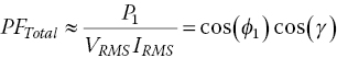
where ![]() .
.


Figure 13.5 (a) Simplified power triangle in the presence of harmonics (b) Modified power triangle.
We may simplify the expression for the total volt‐amps delivered to the circuit, by defining the harmonic VArs as:


where the harmonic VArs are defined as 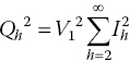 . This quantity is sometimes called the distortion power, and given the symbol D. If we define the total reactive power flowing as QT, where
 ![]() , then we may write
, then we may write ![]() , suggesting the simplified power triangle shown in Figure 13.5a, where the angle Φ is defined by:
, suggesting the simplified power triangle shown in Figure 13.5a, where the angle Φ is defined by:
This equation suggests that the power triangle can be redrawn to include the effect of the harmonic VArs, as shown in Figure 13.5b. The distortion power factor further reduces the total power factor since it increases the RMS current yet does not contribute to the power delivered to the load; harmonic currents only increase the network losses.
Note that Figures 13.5a and 13.5b can no longer be related to a phasor diagram, since the harmonic VArs rotate at angular frequencies different from that of the fundamental, and the angle Φ no longer represents the phase shift between the fundamental voltage and current. This diagram does however illustrate the Pythagorean relationship between the quantities concerned, and it is useful from this point of view. Figure 13.6 shows the variation in distortion power factor as a function of THDi; when this reaches 100% cos(γ) = 0.707.

Figure 13.6 Distortion power factor variation with current THD.
Example: Let us consider a numerical example to illustrate these concepts. The table below shows data collected from measurements on a small inverter‐driven compact fluorescent lamp, the current of which is rich in harmonics.
Compact fluorescent lamp measured data
| VRMS (V) | IRMS (mA) | Power (W) | Current THD (%) |
| 241 | 140 | 20.2 | 112.6 |
Using the equations above and this small amount of data, the information shown in the following table can be obtained. From the THDi value and the RMS current, the fundamental current I1 can be found. This leads to a quite reasonable displacement power factor of 0.9. However, when the reactive harmonic power is taken into account, the total power factor falls to 0.6. This poor result is largely due to the high harmonic component in the supply current and the harmonic VArs that the lamp thus consumes. The above calculations were possible from just four pieces of information, each available from a handheld power analyser.
Power factor analysis
| Fundamental current | Fundamental reactive power (Q1) |
Fundamental power factor cos(ϕ) |
Total reactive power (QT) |
Total power factor |
| 92.6 mA | 9.67 VArs | 0.9 | 27.02 VArs | 0.6 |
Non‐linear devices exhibiting such poor power factors consume a disproportionately large portion of the network capacity in comparison to the power they consume. Unfortunately some manufacturers occasionally state the displacement power factor, but omit to include the distortion power factor, making their product specifications appear better than they really are.
13.7 Management of Harmonics
The impact that a given distorting load will have on a network depends upon the capacity of the network at the point of connection, which is frequently expressed in terms of the three‐phase short circuit current ISC. Small loads may be defined as those whose maximum demand current is less than 1 per cent of ISC. Many ‘small’ customers are unaware that the harmonic content of their load needlessly increases network losses, but since their contribution is small this is generally of little consequence.
‘Large’ loads, on the other hand, demand currents that represent a considerably larger fraction of ISC, 5 or 10% of ISC for example. ‘Large’ customers must actively manage the effects that their distorting load has on the network, and harmonic emission limits are frequently included in connection agreements in order to enforce this. Harmonic management is often achieved by installing harmonic filters in parallel with the offending load, or by using harmonic cancellation techniques. These involve arranging the load in such a way that current flows smoothly over as much of the AC cycle as possible. Important examples of this appear in the design of electrowinning rectification equipment and variable speed drives (VSDs – also known as adjustable frequency drives, ASDs) where rectifier circuits are often arranged to achieve a high pulse number.
13.7.1 Harmonic Cancellation Techniques (Rectifier Pulse Number)
It is often necessary to rectify the three‐phase AC supply in order to produce a source of DC potential, perhaps for use in a variable frequency drive, a converter circuit or for the electrolytic deposition of metals such as zinc or tin. In all these applications a three‐phase bridge rectifier circuit is commonly used to produce a relatively smooth DC potential.
The circuit depicted in Figure 13.7 is a naturally commutated six‐pulse rectifier, so called because of the use of uncontrolled rectifier diodes to produce a DC waveform containing six ripple pulses per cycle of the fundamental. These switch in a sequence that presents the load with whichever line voltage is instantaneously the most positive; the DC voltage generated being equal to 1.35 times the magnitude of the RMS AC line voltage.

Figure 13.7 Three‐phase bridge rectifier and voltage waveforms.
Figure 13.8 shows the diode and line currents for a rectifier supplied from a set of star connected windings, each conducting for 120° every half cycle. When the rectifier is supplied from a delta connected set, the line current adopts the stepped waveform shown in Figure 13.9 and flows continuously throughout each cycle.

Figure 13.8 Star connected three‐phase rectifier line voltages, line current and harmonic spectrum.

Figure 13.9 Typical construction of a twelve‐pulse rectifier.
The AC line current of either rectifier configuration contains harmonics of order np ± 1, where p is the pulse number (in this case six), and n is a positive integer. Thus a six‐pulse rectifier’s line current includes 5th and 7th harmonics as well as 11th and 13th, 17th and 19th and so on, as shown in Figure 13.8. As the harmonic number h increases, so the harmonic current amplitude decreases, in roughly inverse proportion.
Although the amplitude spectrum is the same for each winding configuration, the phase spectrum is not, and when these line currents are added, a substantial reduction in the lowest harmonics results occurs due to harmonic cancellation. Because of this there is a significant benefit to be gained from using a rectifier with a high pulse number, since this means that the first harmonic present will have frequency of p − 1 times the fundamental, and if p is sufficiently large, its amplitude will be relatively small. Twelve‐pulse rectifiers are commonly used on this account, and can be built by introducing a 30° phase shift between two six‐pulse rectifiers, as shown in Figure 13.9.
A 30° phase shift is usually achieved by supplying one six‐pulse rectifier from a delta connected transformer winding and the other from a star connected one. The traditional method for combining the outputs of two such rectifiers is to use an inter‐phase transformer (shown in Figures 13.9 and 13.10), which supports the difference between their output voltages while summing their currents. This transformer usually has a single turn winding on each side, made by passing the DC busbars through a transformer core, in much the same way that an AC busbar passes through a current transformer. The busbars are arranged so that the DC currents from the rectifiers flow in opposite directions through the core, avoiding the creation of a DC flux, while supporting the cumulative ripple voltage that exists between them. In this way, each rectifier continues to operate as an independent six‐pulse unit, while the output voltage and current of the combination appear as twelve‐pulse.

Figure 13.10 A 20 kA inter‐phase transformer used in a small electrolytic zinc plant.
Modern electrolytic rectifiers generally do not employ inter‐phase transformers; they rely instead on the reactance of the outgoing DC busbars across which to drop the difference in ripple voltages. For this approach to be successful, these busbars must be of sufficient length and each must only carry the current from one rectifier bridge.
Figure 13.11 shows the effect of adding the winding currents from each six‐pulse bridge, the combination of which provides a considerably smoother line current. The twelve‐pulse harmonic spectrum begins at the 11th harmonic and, as mentioned, contains components at ![]() times the fundamental frequency. However, as shown in the figure, the degree of cancellation of the 5th and 7th harmonics depends on the precision of the matching between the component rectifiers. When the star and delta bridges are not precisely matched in terms of DC voltage and current, residual 5th and 7th harmonic currents may remain, although these will generally be much lower in amplitude than those of the 11th and 13th.
times the fundamental frequency. However, as shown in the figure, the degree of cancellation of the 5th and 7th harmonics depends on the precision of the matching between the component rectifiers. When the star and delta bridges are not precisely matched in terms of DC voltage and current, residual 5th and 7th harmonic currents may remain, although these will generally be much lower in amplitude than those of the 11th and 13th.


Figure 13.11 Harmonic cancellation in a twelve pulse rectifier.
Similar arrangements are used in the design of variable speed drives (VSDs), where a variable frequency three‐phase system is synthesised from a DC voltage produced by rectifying the incoming AC supply. Low voltage drives often use 12‐ or 18‐pulse rectifiers instead of a 6‐pulse bridge, while medium voltage drives frequently use 24‐pulse rectifiers in order to reduce the supply current distortion to acceptably low levels.
However, this harmonic cancellation concept can be extended much further. Aluminium and zinc producers, for example, frequently pass DC currents in excess of 200 kA through their electrolytic cells. Currents of this magnitude are traditionally obtained from a fleet of naturally commutated rectifiers, each one phase shifted from the others by a small angle, so that when seen from the supply side, a very high pulse number results. For example, when a fleet of six 12‐pulse rectifiers is employed, each phase shifted from its neighbours by 5°, a pulse number of 72 results. The first significant harmonics are the 71st and the 73rd, and as a result the resulting line currents will be almost sinusoidal, since the amplitudes of these harmonics will be very low.
13.7.2 Harmonic Filters
In the past three decades there has been a move away from naturally commutated rectifiers for electrolytic plants towards thyristor controlled rectifiers. Thyristors provide the ability to adjust the DC output voltage by delaying the point on the line voltage waveform at which each thyristor fires (i.e. by controlling its firing angle). This avoids the expense and complexity of an on‐load tap‐changer within the transformer tank.
Because both the amplitude and phase of current harmonics in controlled rectifiers are strongly influenced by the firing angle, the phase shifting techniques described above are generally not successful, since small differences in firing angles will result in incomplete harmonic cancellation. As such, achieving a high pulse number will not provide a reliable means of harmonic reduction. Instead it is usual to install a harmonic filter on the supply bus, close to the rectifier, to provide a path to ground for harmonic currents that would otherwise flow into the upstream network.
There are also many other large industrial devices connected to the power system today, including inverters, static VAr compensators (SVCs), cycloconverters, DC Motor controllers and high voltage DC (HVDC) transmission equipment, all of which employ thyristors or insulated gate bipolar transistors (IGBTs). This equipment also consumes currents rich in harmonics and it is often necessary to install harmonic filtering equipment to suppress the harmonic currents that would otherwise flow into the local network. There are various harmonic filter circuits used for this purpose, but we will consider one of the more common, the series tuned LC circuit, which is designed to provide a current sink at a discrete harmonic frequency.
Figure 13.12a shows a typical single stage series resonant harmonic filter used to sink non‐triplen harmonic currents. The series connected tuning inductances supply two star connected sets of capacitors, collectively resonant just below the target harmonic. This circuit presents a low impedance at the target frequency and thus provides a local sink for harmonic currents. The filter’s single‐phase equivalent circuit appears in Figure 13.12b, the resistive component of which (Rf) represents the losses associated with the tuning reactors.

Figure 13.12 (a) Typical schematic for a harmonic filter (b) Single‐phase equivalent circuit.
The capacitors are frequently split into two star connected groups as shown, with a balance current transformer inserted between the star points. So long as both star networks remain balanced, there will be no current flowing in this CT. However, if a partial capacitor failure occurs in one or more phases (usually as a result of the open‐circuiting of one or more of the internal capacitive elements), then a proportional unbalance current will flow in the CT. Small currents will not warrant tripping the filter and may simply raise an alarm, but a complete capacitor failure will result in a large current flow, requiring the immediate tripping of the filter.
Series and Parallel Resonance
A typical impedance plot for a 50 Hz high voltage 5th harmonic filter appears in Figure 13.13. The series resonant frequency (or notch frequency) is determined solely by the filter components and is given by:

Figure 13.13 Impedance plot of a 50 Hz single stage HV 5th harmonic filter.
In this example fseries is 240 Hz.
The local source inductance Ls appears in parallel with the filter elements, and it therefore creates a parallel tuned circuit, resonant just a little below the target frequency. The parallel resonant frequency is given by Equation (13.13b), occurring in this case at about 208 Hz.
While externally a parallel resonant circuit appears as an open circuit, internally there can be very large currents exchanged between the inductance and capacitance, particularly if the Q of the circuit is high. The danger of parallel resonance occurring at or near an active harmonic must be taken into account when installing harmonic filters or power factor correction capacitors. This is because large and destructive currents can be exchanged between the filter capacitance and the source should a parallel resonance be excited by harmonic currents already present in the network. Should such a situation occur, the capacitors will usually experience a substantial over voltage, usually followed by rapid failure.
The series resonant circuit is generally tuned a little below the target harmonic, since this will permit a partial capacitor or inductor failure without permitting the circuit’s resonant frequency to rise significantly above the target harmonic. Were this to occur, then the target harmonic may fall close to the parallel resonant frequency, presenting the possibility that the harmonic will be amplified as a result.
Away from these resonant frequencies, the filter’s impedance rises significantly with respect to that of the source, thus in these regions the network impedance is dominated by the inductive component of the source, scaled according to frequency. This effect is shown by the dotted line in Figure 13.13, which represents the system impedance in the absence of the filter.
Distorting loads frequently generate current at several harmonic frequencies, and therefore require the use of multi‐stage harmonic filters. Figure 13.14 shows the frequency response of a medium voltage, four‐stage 50 Hz series tuned LC filter, including the connected load.

Figure 13.14 Frequency response of a 50 Hz four‐stage MV harmonic filter and load.
In this example, the stages are tuned to the 5th, 7th, 11th and 13th harmonics, each corresponding to a notch in the response. Between adjacent notch frequencies lies a parallel resonance. In this case, most are not particularly sharp, due to the damping effect of the load, but each could give rise to unwanted harmonic amplification. Fortunately, the parallel resonant frequencies all lie close to even harmonics where little or no harmonic energy is expected.
Figure 13.14 illustrates an important point: whenever it is necessary to introduce a notch frequency into the spectrum, an associated parallel resonance will always occur a little below it, one that must not coincide with an active harmonic. For example, if the 7th harmonic current is to be targeted with a series tuned filter, it is usual to also install a 5th harmonic filter as well, so as to force a low system impedance at the 5th harmonic, and hence avoid any parallel resonance that may otherwise occur there.
The installation of power factor correction and voltage support capacitors also gives rise to parallel resonant frequencies. It is usual therefore to include a de‐tuning reactance in such circuits to ensure that the parallel resonant frequency does not lie near an active harmonic. This reactance is chosen so that the series resonant frequency generally lies well below the 5th, thereby preventing 5th harmonic currents from overloading the capacitors. Such circuits are said to be de‐tuned. The de‐tuning reactance is also useful in limiting the transient inrush current that flows into the capacitors at switch on. Its impedance is usually expressed in terms of the de‐tuning ratio p, which is given by:

where XL is the reactance of the inductor at the fundamental and XC is the reactance of the capacitance at the fundamental.
Thus if p = 7% the reactor impedance is 7% of that of the capacitor at the fundamental frequency. The series resonant frequency is given by:

where L is the reactor inductance, C is the effective capacitance, f1 is the fundamental frequency and p is the de‐tuning ratio.
Table 13.6 shows some commonly used series resonant frequencies in the application of power factor correction and voltage support capacitances.
Table 13.6 Common series resonant frequencies used for voltage support and PFC capacitors.
| Series resonant frequency (50 Hz systems) |
Series resonant frequency (60 Hz systems) |
De‐tuning ratio p (% of Xc at the fundamental) |
| 134 Hz | 160 Hz | 14 |
| 189 Hz | 227 Hz | 7 |
| 204 Hz | 245 Hz | 6 |
| 210 Hz | 252 Hz | 5.67 |
Triplen harmonics are eliminated from harmonic filters and PFC equipment by connecting the capacitors in an ungrounded star configuration, as is usually the case in MV distribution networks, or by using a delta connection, as is generally found in LV applications.
Active Harmonic Filters
While passive harmonic filters are robust and require little maintenance, they modify the system impedance spectrum and are generally only able to target a discrete range of harmonic frequencies. Active filters on the other hand can target all harmonics up to about the 50th without introducing changes to the impedance spectrum. They are essentially semiconductor converter circuits connected in parallel with an offending load, as shown in Figure 13.15. They measure and invert the load’s harmonic content, and by injecting it back onto the bus they cancel the harmonic currents flowing from the load, leaving only the fundamental component in the supply.

Figure 13.15 Active harmonic filter operation.
Because the converter circuit appears as a high impedance current source, the active filter does not modify the system impedance, and therefore does not introduce unwanted resonances. Active filters have a finite current capacity, and therefore must be carefully chosen to suit the harmonic spectrum of the intended load. They are particularly useful for providing harmonic cancellation for a collection of VSDs. They can also be used to provide reactive support at the fundamental, but in this respect they are an expensive way to provide power factor correction.
13.8 Harmonic Standards
The International Electrotechnical Commission publishes the IEC 61000 series of standards on harmonics and power quality, including the following:
- IEC 61000‐3‐2 Limits for harmonic current emissions (equipment input ≤ 16 A per phase)
- IEC 61000‐3‐4 Limits for harmonic current emissions in LV power supply systems for equipment input > 16 A per phase
- IEC 61000‐3‐12 Limits for harmonic equipment currents produced by equipment connected to the public LV system with input current ≥ 16A
- Technical Report IEC 61000.3.6 (2012), Assessment of emission limits for the connection of distorting loads to MV, HV and EHV power systems.
The last document provides an excellent introduction to electromagnetic compatibility and harmonic assessment, and in many countries it carries the weight of a standard, while in others it has been formally adopted as such. In the USA the IEEE Std 519 (2014), IEEE Recommended practice and requirements for harmonic control in electric power systems prescribes the limits for harmonic emissions at all voltage levels.
A detailed analysis of all these documents is beyond the scope of this book; however, we will consider the Technical Report IEC 61000‐3‐6, which explains the broader issues that form the basis for allocating the harmonic absorption capacity of the power system. We will also discuss the current and voltage distortion limits prescribed in IEEE 519, and the conditions under which they apply.
13.8.1 Electromagnetic Compatibility, Planning and Allocation Levels
The electromagnetic compatibility is the ability of all equipment connected to the power system to operate satisfactorily in the presence of disturbances, which may include harmonics and voltage fluctuations, such as voltage notching and flicker. For electromagnetic compatibility to be maintained, the immunity level of the equipment concerned must be greater than the emission levels of the devices creating the disturbance. For the purposes of the present discussion we shall assume that disturbances relate to the effects of harmonic voltage distortion.
The power system generally has a low impedance and as a consequence is relatively well regulated. It is therefore reasonably tolerant of the harmonic currents that are injected by non‐linear loads. Some of these currents add destructively while others accumulate; however, the resulting voltage distortion occurring throughout the network can be kept acceptably low provided customers take steps to ensure that their loads do not exceed the prescribed harmonic allocation limits.
Harmonic currents are in most cases independent of the system impedance and are relatively easily to measure. Harmonic voltage distortion on the other hand contains a background component at each harmonic, as a result of the injection of harmonic currents elsewhere in the network, plus a component produced by currents flowing from each customer’s distorting load through the local network impedance. It is therefore difficult to accurately determine what proportion of the voltage distortion is attributable to any particular customer, unless the network harmonic impedance is known at the connection point. Harmonic impedances can be difficult to predict, particularly when there are capacitors within the local network that may introduce resonances.
The primary intent of harmonic standards is to restrict the harmonic voltage distortion to an acceptable level and to share the harmonic capacity of the network between all present and future customers, roughly in proportion to the size of their connected loads. Rather than allocating a proportion of the permitted harmonic voltage distortion to individual customers, harmonic standards generally limit the magnitude of harmonic currents that may be injected instead, thus avoiding the need to determine the harmonic impedance associated with each customer connection.
One consequence of an excessive level of harmonic voltage distortion is the mal‐operation of some items of customer equipment, in either the LV or MV networks. Because harmonic voltage distortion is a continuously varying quantity, a statistical approach is adopted in its measurement. This is expressed in terms of the probability density curves shown in Figure 13.16a, which depict the relationship between the local equipment immunity levels and the site disturbance level produced by non‐linear loads in a particular locality. The area beneath the immunity probability density curve to the left of a particular disturbance level represents the probability that the equipment will be disrupted by that disturbance. In this case, the disturbance level can be thought of as the magnitude of a given harmonic, expressed as percentage of the fundamental.


Figure 13.16 (a) Site disturbance levels (b) Global disturbance levels (IEC/TR 61000‐3‐6 ed.2.0 Copyright © 2008 IEC Geneva, Switzerland. www.iec.ch).
In the context of a particular location in a network we expect that the likelihood of overlap between the disturbance and immunity distributions will be small or non‐existent, and that a suitable planning level can easily be chosen for any particular harmonic that will not result in local equipment malfunction. This situation is depicted in Figure 13.16a.
On the other hand when viewed globally, the entire network may experience a small overlap between disturbance and immunity levels, as shown in Figure 13.16b. This is in recognition of the fact that the network owner cannot control the harmonic levels at all locations throughout the network, all of the time. The immunity to a particular disturbance of a piece of equipment is a function of its design, and immunity test levels are usually agreed upon between manufacturers and users, to ensure acceptable product performance.
The compatibility level is used by the network owner to determine the electromagnetic compatibility of the entire network, and may be thought of as an upper bound to the planning level. It is based on the 95% disturbance level of the network, meaning that for 95% of the time the disturbance level will be less than the measured value.
The planning levels for harmonic voltages or currents are usually set by the network owner, and may vary slightly from one location to another, although in some countries they are prescribed in national standards. They can be considered as internal quality objectives for the network and vary with the harmonic number and the voltage level concerned. They will always be less than or equal to the associated compatibility level. The compatibility and indicative planning levels for individual harmonic voltages appear in Tables 13.7 and 13.8.
Table 13.7 LV and MV compatibility limits.
(IEC/TR 61000‐3‐6 ed.2.0 Copyright © 2008 IEC Geneva, Switzerland. www.iec.ch)
| Odd, non‐triplen harmonics | Triplen harmonics | Even harmonics | |||
| Harmonic order (h) | Harmonic voltage (%) | Harmonic order (h) | Harmonic voltage (%) | Harmonic order (h) | Harmonic voltage (%) |
| 5 | 6 | 3 | 5 | 2 | 2 |
| 7 | 5 | 9 | 1.5 | 4 | 1 |
| 11 | 3.5 | 15 | 0.4 | 6 | 0.5 |
| 13 | 3 | 21 | 0.3 | 8 | 0.5 |
| 17 ≤ h ≤ 49 | |
21 ≤ h ≤ 45 | 0.2 | 10 ≤ h ≤ 50 | |
| The compatibility level for the total harmonic distortion (THD) is 8% | |||||
Table 13.8 MV, HV and EHV indicative planning limits.
(IEC/TR 61000‐3‐6 ed.2.0 Copyright © 2008 IEC Geneva, Switzerland. www.iec.ch)
| Odd, non‐triplen harmonics | Triplen harmonics | Even harmonics | ||||||
| Harmonic order (h) |
Harmonic voltage (%) |
Harmonic order (h) |
Harmonic voltage (%) | Harmonic order (h) |
Harmonic voltage (%) | |||
| MV | HV & EHV |
MV | HV & EHV | MV | HV & EHV |
|||
| 5 | 5 | 2 | 3 | 4 | 2 | 2 | 1.8 | 1.4 |
| 7 | 4 | 2 | 9 | 1.2 | 1 | 4 | 1 | 0.8 |
| 11 | 3 | 1.5 | 15 | 0.3 | 0.3 | 6 | 0.5 | 0.4 |
| 13 | 2.5 | 1.5 | 21 | 0.2 | 0.2 | 8 | 0.5 | 0.4 |
| 17 ≤ h ≤ 49 | |
|
21 ≤ h ≤ 45 | 0.2 | 0.2 | 10 ≤ h ≤ 50 | |
|
| Indicative planning levels: THDMV = 6.5% and THDEHV = 3% | ||||||||
For very short disturbances of 3 seconds or less, both the compatibility and the indicative planning levels may be increased by a factor khvs, where:
These tables are divided into three classes of harmonic: odd non‐triplen harmonics, odd triplen harmonics and even harmonics. Even harmonics will not usually be present in the network due to the preponderance of half wave symmetry, and as a consequence the compatibility levels are set somewhat lower than for the other classes. Odd non‐triplen harmonics generally represent the majority of system disturbances, particularly in the lower orders, and therefore the levels specified are considerably higher than for even harmonics. Note that as the harmonic order increases the compatibility level decreases, in a similar way to which harmonic amplitudes themselves tend to decrease. Odd triplen harmonics are in a class of their own. Of these the third is the most important since it can exist in LV and to a lesser extent in some MV networks. At higher orders, odd triplen harmonics generally exist only at small amplitudes, hence the reduction in level beyond the 9th.
The emission limit (sometimes called the allocation level) is the maximum permitted disturbance level imposed on an individual customer’s load, usually specified as part of the network connection agreement. It is generally a fraction of the local planning level, and is chosen in proportion to network capacity consumed by the load. The allocation level is effectively an upper bound to the emissions permitted from the load in question.
13.8.2 IEEE Std 519 IEEE Recommended Practice and Requirements for Harmonic Control in Electric Power Systems
IEEE Std 519 is principally concerned with ensuring that the network voltage distortion limits are maintained. It specifies acceptable voltage distortion limits (THDv) for all network phase voltages at the point of common coupling (PCC) between the customer concerned and the local network; these are shown in Table 13.9.
Table 13.9 IEEE 519 Voltage harmonic distortion limits.
(Adapted and reprinted with permission from IEEE. Copyright IEEE 519 (2014). All rights reserved. Permission for further use of this material must be obtained from IEEE. Requests may be sent to stds‐[email protected])
| Bus voltage at the PCC | Individual harmonic (% of fundamental) |
THDv (%) |
| V ≤ 1 kV | 5.0 | 8.0 |
| 1 kV < V ≤ 69 kV | 3.0 | 5.0 |
| 69 kV < V ≤ 161 kV | 1.5 | 2.5 |
| V > 161 kV | 1.0 | 1.5 |
The point of common coupling is the closest point in the network to the customer connection at which other customer(s) are or could be connected. For many customers this will generally be the low voltage bus from which the supply originates and from which other customers are supplied, but for LV customers supplied from a dedicated MV transformer, the PCC lies at the point of connection to the MV network. This distinction is important since the standard must only be complied with at the PCC, and not necessarily throughout the customer’s plant, where LV harmonic levels are likely to be considerably higher.
Provided that the network owner ensures that all customers adhere to these limits, then the absorption capacity of the network should be such that the voltage limits will be met. IEEE Std 519 permits the limits in Table 13.9 to be exceeded in the very short term (3 seconds). Voltage harmonics exceeding the daily 99th percentile (i.e. those exceeded only 1% of the time) very short time values must be less than 150% of those given in the table. The weekly 95th percentile short time (10 minutes) values, however, must be less than those in the table.
As previously mentioned, it is difficult to accurately apportion voltage harmonic distortion to any particular customer. IEEE Std 519 recognises this by defining limits to the harmonic currents that a given load can inject into the network. The current distortion limits for system voltages between 120 V and 69 kV are given in Table 13.10. These are defined in terms of the short circuit ratio which is defined as the ratio of the short circuit current at the PCC to the maximum demand current of the load concerned: ISC/IL. The standard defines IL as the sum of the maximum demand current measured in each of the proceeding twelve months, divided by 12. Table 13.10 also imposes additional restrictions on the harmonic spectrum of the load by limiting the maximum total demand distortion.
Table 13.10 IEEE 519 current distortion limits for system voltages between 120 V and 69 kV.
(Adapted and reprinted with permission from IEEE. Copyright IEEE 519 (2014). All rights reserved. Permission for further use of this material must be obtained from IEEE. Requests may be sent to stds‐[email protected])
| Maximum harmonic current distortion (% IL) (Individual odd order harmonics) |
||||||
| I SC /IL | 3 ≤ h < 11 | 11 ≤ h < 17 | 17 ≤ h < 23 | 23 ≤ h < 35 | 35 ≤ h ≤ 50 | TDD |
| I SC /IL < 20 | 4.0 | 2.0 | 1.5 | 0.6 | 0.3 | 5.0 |
| 20 < ISC/IL < 50 | 7.0 | 3.5 | 2.5 | 1.0 | 0.5 | 8.0 |
| 50 < ISC/IL < 100 | 10.0 | 4.5 | 4.0 | 1.5 | 0.7 | 12.0 |
| 100 < ISC/IL < 1000 | 12.0 | 5.5 | 5.0 | 2.0 | 1.0 | 15.0 |
| I SC /IL > 1000 | 15.0 | 7.0 | 7.0 | 2.5 | 1.4 | 20.0 |
| Even harmonics are limited to 25% of the values listed above | ||||||
Small loads for which the short circuit ratio is large consume relatively little network capacity and therefore can be permitted to inject a larger relative proportion of harmonic current. On the other hand, large loads with small short circuit ratios consume much more network capacity and are therefore considerably more restricted in terms of the harmonic currents they can inject.
The daily 99th percentile very short time harmonic currents must be less than twice the levels given in Table 13.10, while the weekly 99th percentile short time currents must be less than 150% of these limits. Finally, the weekly 95th percentile short time currents must be less than 100% of the limits in the Table 13.10.
13.8.3 Assessment of MV Customer Emission Levels
IEC 61000.3.6 defines three stages of assessment, which are used in sequence to decide if a particular distorting load may be connected to the MV network without exceeding the local planning levels. Small distorting loads may well pass stages 1 or 2, and thus may be connected with relatively little detailed analysis. However, larger loads often require detailed system studies to determine the pre‐existing harmonic levels at the PCC and suitable emission limits and the conditions under which the connection may be permitted.
The Australian publication, Handbook 264 Power quality recommendations for the application of AS/NZ 61000.3.6 and AS/NZ 61000.3.7 provides more information as well as numerical examples for stage 1, 2 and 3 assessments. This is an excellent source of information to which the interested reader is referred. The main requirements of each stage are described below.
Stage 1 Assessment
The stage 1 assessment is similar to the short circuit ratio approach employed in IEEE 519. It is based on the customer’s agreed power consumption Si (which will usually be defined in terms of the contract maximum demand), relative to the system short circuit fault level at the point of common coupling, Ssc. If ![]() then the distorting load may be connected without further investigation. If this inequality is not satisfied then a weighted summation of the customer’s distorting loads may be computed, to produce an effective distorting power, SDwi where:
then the distorting load may be connected without further investigation. If this inequality is not satisfied then a weighted summation of the customer’s distorting loads may be computed, to produce an effective distorting power, SDwi where:
where SDj is the power of distorting equipment j of customer i, and Wj is a load dependent weighting factor, some of which appear in Table 13.11.
Table 13.11 Harmonic weighting factors for some common MV loads.
(IEC/TR 61000‐3‐6 ed.2.0 Copyright © 2008 IEC Geneva, Switzerland. www.iec.ch)
| Equipment | Typical THD (%) | Weighting factor (Wj) |
| 6‐pulse converter with capacitive filtering | 80 | 2.0 |
| 6‐pulse converter with capacitive and partial inductive filtering | 40 | 1.0 |
| 6‐pulse converter with heavily inductive load | 28 | 0.8 |
| 12‐pulse converter | 15 | 0.5 |
If the ratio of the customer’s weighted distorting power to the system short circuit power is less than 0.2%, then connection of the load is permitted without further investigation.
Stage 2 Assessment
Stage 2 assessments allow for higher emissions than stage 1, based on the capacity of the wider MV network to absorb harmonic currents through diversity and harmonic cancellation. The limits allocated to each customer are commensurate with the fraction of the total available power from the PCC.
Stage 2 offers two approaches to harmonic assessment. The first applies to customers with an agreed power Si less than 1 MVA, on condition that Si/Ssc is less than 1%, and the background harmonic levels are acceptably low. It assigns limits to the harmonic currents that the customer may inject in a similar fashion to those imposed by IEEE 519. Table 13.12 shows some typical limits for odd harmonics as a function of the current corresponding to the customer’s agreed power, IL.
Table 13.12 Indicative emission limits for stage 2 assessments.
(IEC/TR 61000‐3‐6 ed.2.0 Copyright © 2008 IEC Geneva, Switzerland. www.iec.ch)
| Harmonic order h | 5 | 7 | 11 | 13 | >13 |
| Emission limit Ih/IL (%) | 5 | 5 | 3 | 3 | 500/h2 |
The second approach that may be adopted under stage 2 is based on the general summation law defined by Equation (13.15). We are already familiar with this concept from Equation (13.1) in the calculation of the RMS value of a current (or voltage) comprising a series of harmonics. The general summation law is used for the aggregation of harmonic emissions (either voltages or currents) of order h and can be written as:
where Uhi is the magnitude of component i of the harmonic voltage (or current) of order h, Uh is the probabilistic magnitude of the aggregated harmonic voltage (or current) order h and α is the summation exponent given in Table 13.13, and depends on variation in the phase and magnitude of the individual harmonic.
Table 13.13 Harmonic summation exponents.
(IEC/TR 61000‐3‐6 ed.2.0 Copyright © 2008 IEC Geneva, Switzerland. www.iec.ch)
| Harmonic order h | α |
| h < 5 | 1 |
| |
1.4 |
| h > 10 | 2 |
Low‐order odd harmonics have phase angles that vary little across the power system and therefore the chance of cancellation is limited, and as a result α is chosen conservatively for these frequencies. On the other hand higher order harmonics generally vary considerably in both magnitude and phase, offering more scope for cancellation, and therefore are assigned less conservative exponents.
While Equation (13.15) applies to harmonic emissions corresponding to a particular voltage level, it is also useful in combining quantities from different levels. For example, it can be used to aggregate the LV emissions transferred into the MV network.
The second approach defined under stage 2 apportions each customer a fraction of the global voltage emission limit ![]() of the total MV and LV load that can be supplied from the MV bus in question, according to:
of the total MV and LV load that can be supplied from the MV bus in question, according to:

where EUhi is the harmonic voltage emission limit of order h for distorting MV load i, Si is the agreed power the distorting load, St is the total MV supply capacity, including any associated LV loads and α is the harmonic exponent, enabling smaller loads to receive a larger relative allocation.
The MV planning level for harmonic h (LhMV) is expressed using the general summation law as the vector summation of the MV harmonic voltage distortion plus that contribution transferred from the upstream HV network (which is assumed to have already reached its planning level), thus:
where ThUM is the transfer coefficient of harmonic voltage distortion from the upstream network to the MV network. This typically has a value around unity, although it may be as high as 3 in the presence of harmonic resonances.
From this equation we obtain the global contribution ![]() for the combined MV and LV load:
for the combined MV and LV load:
Provided the load concerned can meet the limits defined by Equation (13.16) it may be connected without further investigation. Equation (13.16) provides an emission limit in terms of the voltage distortion at the PCC for harmonic h, rather than in terms of the current that can be injected at each significant harmonic, which is generally much more useful to the customer. If the harmonic impedance at the PCC is known, the corresponding current emission limit EIhi can be found since ![]() , where Zhi is the system impedance at harmonic h of customer i.
, where Zhi is the system impedance at harmonic h of customer i.
As mentioned earlier, harmonic impedances can be difficult to predict, especially when resonances exist in a network. At locations where there are no connected capacitances, low‐order harmonics Zhi can often be approximated by hx1, where x1 is the fundamental short circuit reactance at the PCC. This parameter will vary with changes in network configuration and it is best to err on the high side if a conservative approach is to be adopted. IEC 61000.3.6 suggests that for h < 8 an upper bound to Zhi is ![]() .
.
Loads connected close to the HV‐MV interface will generally see relatively low harmonic impedances, and can be allocated emission levels according to Equation (13.16). However, loads connected to long MV feeders remote from the MV bus, will experience considerably higher source impedances and proportionally lower short circuit currents. For similar agreed power levels these customers will therefore receive lower harmonic current allocations than those nearer the sending end.
Alternatively, the allocation of equal harmonic currents to all such customers would require low emissions limits in order to contain the voltage distortion at the far end of the line, in which case the network’s capacity to absorb harmonic currents would be under‐utilised. IEC 61000.3.6 suggests that, in these situations, an allocation based on harmonic VA be used instead; the current emission limit being given by:

where AhMV is the allocation constant, chosen for a given network, so that the planning level on the weakest feeder is preserved.
In this case, the harmonic current allocation is inversely proportional to ![]() . The interested reader is referred to IEC 61000.3.6, Annex B, which includes examples of this approach.
. The interested reader is referred to IEC 61000.3.6, Annex B, which includes examples of this approach.
Stage 3 Assessment
Equation (13.16) suggests that if all customers contribute no more than their share of the planning level at each harmonic, then the planning levels will not be exceeded. However, it is known that some customers generate very few harmonics, as a result of largely linear loads. Because of this, the strict use of Equation (13.16) will generally lead to voltage harmonic levels significantly below the planning levels.
The network owner therefore generally has some discretion to permit new customers to exceed the limits that would normally be imposed, and in so doing use some of the excess capacity within the network. Stage 3 assessments require a detailed study of the network background levels at the PCC as well as of the expected contribution of the new load, under various network configurations. Connection to a network under a stage 3 assessment may be on a conditional basis, thus postponing harmonic mitigation investment by the customer or possibly restricting the operation of distorting loads under certain network configurations.
13.9 Measurement of Harmonics
The assessment of the background harmonic levels present on a bus is always advisable prior to the connection of a large distorting load, i.e. one for which ![]() . Such measurements can avoid subsequent arguments as to whether the contribution to the bus distortion by the new load is excessive. Standards IEEE 519 and IEC61000.3.6 both specify limits up to the 50th harmonic; however, accurate measurement of these may not always be possible with conventional voltage transformers. Capacitive VTs (CVTs) for example are tuned to the fundamental frequency and are therefore only accurate over a very narrow range of frequencies on either side of it. Inductive VTs may also exhibit resonances as low as 500 Hz, due to parasitic winding capacitances and, depending on the applied burden, are also likely to misreport harmonic levels.
. Such measurements can avoid subsequent arguments as to whether the contribution to the bus distortion by the new load is excessive. Standards IEEE 519 and IEC61000.3.6 both specify limits up to the 50th harmonic; however, accurate measurement of these may not always be possible with conventional voltage transformers. Capacitive VTs (CVTs) for example are tuned to the fundamental frequency and are therefore only accurate over a very narrow range of frequencies on either side of it. Inductive VTs may also exhibit resonances as low as 500 Hz, due to parasitic winding capacitances and, depending on the applied burden, are also likely to misreport harmonic levels.
Unless the actual frequency response is known and can be corrected for, the installed VTs generally should not be relied upon when making harmonic measurements, and non‐conventional voltage transformers should be considered instead. These could be RC based voltage divider instruments or perhaps an optical VT, and may need to be installed for the measurement period. It is also possible to measure and integrate the current flowing in the capacitive divider of a CVT, in order to produce a faithful replica of the voltage spectrum, including at least the first 50 harmonics. Proprietary equipment is available for this purpose, which can be retrospectively fitted to most capacitive voltage transformers.
Where injection limits are based on current harmonic content, soon after a load is connected its harmonic content should be measured to ensure compliance with the prescribed limits (such as those in Table 13.10). In this regard, conventional inductive current transformers will usually be quite adequate for harmonic frequencies up to the 50th. If required, higher‐order harmonics should perhaps be measured with a non‐conventional current transformer such as a Rogowski coil, which will provide a considerably broader frequency response.
Measurement Periods and Target Frequencies
The standards require that harmonic measurements be made over very short intervals of 3 seconds and short intervals of 10 minutes. These should be accumulated over a period of one day and one week respectively. The 99th percentile of the very short time values and the 95th percentile of the short time values are then compared with the harmonic voltage or current limits, as described in Section 13.8.2.
Measurements should be made at times when the maximum harmonic disturbance is expected, i.e. when all distorting loads are in operation. The harmonic frequencies measured shall include, at a minimum, the 3rd, 5th and 7th, in addition to any harmonic frequencies specific to the equipment concerned. The latter, for example, will include the resonant frequencies of any harmonic filters present, or in the case of high pulse number converters, frequencies equal to (np ± 1), where p is the pulse number and n is an integer.
Where the harmonic limits are based on the contribution to the harmonic voltage distortion at the PCC, the local network configuration should also be considered when harmonic measurements are to be made. Equipment outages, for example, may temporarily leave a network in a state of reduced fault level, yielding an apparently higher system impedance. This will tend to accentuate the harmonic voltage distortion created by the load beyond the level that might normally be expected.
Very Short Time Measurements (3 Seconds)
Voltage or current measurements are generally made using a fast Fourier transform (FFT) technique. Instruments should be synchronised to the fundamental frequency and should sample the respective waveform over a period of about 200 ms, recording the value of each harmonic. The RMS averaging process shown in Equation (13.17) is then used over 15 consecutive intervals to obtain a 3‐second very short time harmonic voltage value.

where Vn, vs is the very short (vs), 3‐second RMS value of the nth harmonic voltage. A similar equation applies for harmonic currents.
Short Time Measurements (10 Minutes)
A 10‐minute harmonic voltage value can be obtained by similarly averaging 200 consecutive 3‐second values as shown in Equation (13.18).

where Vn, sh is the short (sh), 10‐minute RMS value of the nth harmonic voltage. A similar equation applies for harmonic currents.
13.10 Problems
- 1 Derive Equation (13.1). Does this equation hold when the currents are not harmonically related but are arbitrary sinusoids instead?
- 2
- Show that where half wave symmetry exists then
 for k even, and for k odd that
  .
. - Show that when i(t) is an even function, the bk terms become zero.
- Show that when i(t) is an odd function, the ak terms become zero.
- Show that where half wave symmetry exists then
- 3 In this question, we consider the cancellation of the 5th and 7th harmonics in the 12‐pulse rectifier configuration shown in Figure 13.9. The 30° phase shift required between the two rectifier bridges is achieved by using Dd0 and Dy11 connected transformers. The Dd0 connection introduces no phase shift between HV and LV windings, but the Dy11 connection introduces a 30° leading phase shift, as seen by the LV windings. Each 6‐pulse rectifier functions entirely independently, emitting harmonic currents of order
 . Therefore we may notionally express the AC current flowing in the LV delta winding in the form:

where Ii is the amplitude of harmonic i (and may be negative).
- Write a similar expression for the LV star winding current, taking into account the 30° phase shift introduced by the Dy11 connection.
- These currents are reflected into the HV windings of their respective transformers, and collectively make up the supply line current. The Dd0 transformer presents a scaled version of IΔ, but the Dy11 transformer introduces a 30° phase shift, the sign of which is dependent on the phase sequence of the harmonic concerned. It can be shown that the Dy11 connection introduces a 30° leading phase shift for positive sequence voltages from HV to LV, and a 30° lagging phase shift for negative sequence voltages, a characteristic possessed by half of the harmonics present. Demonstrate this using phasor diagrams similar to those in Figure 7.7.
- Therefore the summation of the HV currents depends upon the sequence of the harmonics concerned, and can be expressed as follows:
 for positive sequence harmonics (1st, 4th, 7th, 10th, 13th…) and
  for negative sequence harmonics (2nd, 5th, 8th, 11th, 14th…)
- 4 A 6.6 kV pump motor is supplied from a dedicated 22 kV:6.6 kV transformer, shown in Figure 13.17. The motor is supplied from a 6‐pulse VSD demanding 1500 kVA and having a displacement power factor of 0.85. The fault level at the 22 kV bus is 50 MVA and there are no nearby capacitors. A slightly pessimistic estimate for the harmonic emissions from the VSD suggests that
 .
.

Figure 13.17 Pump motor supply.
- Determine the total power factor of the load seen at the 6.6 kV bus. Consider harmonics up to and including the 13th.(Answer: 0.82)
- Find the source impedance seen at the 6.6 kV bus in ohms. (Assume for simplicity that all impedances are reactive.)(Answer: 2.45 ohms)
- 5 We now consider the steps necessary to design a 50 Hz, 5th harmonic filter to suit the distorting load in question 4. The filter will be star connected and configured like that in Figure 13.12a and will provide power factor correction for the load while reducing the 5th harmonic emissions to within the limits prescribed by IEEE 519. It is to be tuned to the 4.8th harmonic (i.e. to a frequency 4.8 times the fundamental, just below the 5th harmonic).
- The filter’s reactive power rating is usually chosen so that the load/filter combination achieves an acceptable power factor. Determine the fundamental reactive power required from the filter to increase the combined load’s displacement power factor to 0.95, and hence find the filter’s impedance XF, at the fundamental frequency. (Answer: QF = 371 kVar, XF = 117.4 ohms)
- Show that the capacitive reactance of the filter at the fundamental, XC is related to XF according to:
 , and hence find XC.(Answer: 122.7 ohms)
 - Show also that the filter inductor’s fundamental reactance XL, is given by
 , where h is the harmonic order of the filter (in this case 4.8), and thus obtain XL. (Answer: XL = 5.32 ohms)
Figure 13.18 shows the equivalent circuit with the filter installed. The harmonic currents divide between the filter impedance and that of the source. As expected, the largest harmonic current absorbed by the filter will be the 5th; however, it will also absorb other harmonic components in proportion to the filter and source impedances.
- Assuming that the harmonic spectrum remains as specified in question 4, calculate the magnitude of each harmonic current (up to and including the 13th) flowing into the filter as well as those flowing into the upstream supply. Find the RMS current supplying the combined load.(Answer: IRMS = 118.4 A)
- The capacitor’s voltage rating is not assessed according to the RMS summation of the fundamental plus the harmonic voltage components, as one might expect. Instead the arithmetic sum of these components is used to approximate the peak voltage that the capacitor must sustain and thus to provide a degree of redundancy in the selection of the capacitor’s voltage rating. Therefore to obtain the capacitor voltage rating we use the equation:
The fundamental voltage will influence the capacitor rating to a large extent, and therefore the maximum likely fundamental voltage should be used in this assessment. Find the largest fundamental current flowing through the filter, occurring when the local bus voltage is at a maximum of 1.1 pu, and hence determine the largest fundamental voltage appearing across the capacitor. (Why is this larger than the supplied phase voltage?)

(Answer: I1max = 35.7 A, Vphase = 4380 V)
- From the amplitudes of the harmonic currents evaluated in part (d), obtain the capacitor voltage rating for this filter. Determine also the capacitance value required for each capacitor can.(Answer: Vrated = 5165 volts; C = 13 μF (50 Hz), C = 10.8 μF (60 Hz))
- For this application the reactors will probably be individually constructed on gapped iron cores, and at the 5th harmonic they can be expected to have a Q value of about 50. In addition to the inductance value, the RMS winding voltage rating must also be specified. This is calculated using a similar equation to that used for the capacitor rating:
Calculate the inductance and value required and the winding voltage rating. (Answer: L = 16.9 mH (50 Hz), 14.1 mH (60 Hz); Vrated = 1590 V)

- Show that the filter reduces the level of the 5th harmonic to within the limits imposed by IEEE 519.

Figure 13.18 Division of harmonic currents.
- 6 If the transformer in question 4 is a dry type, calculate the harmonic loss factor (FHL) and the de‐rating factor necessary as a result of the load’s harmonic content:
- for the load without the filter
- for the combined load.
Assume that the magnitude of the rated eddy current loss at the fundamental frequency is 12% of the rated I2R loss.
(Answer: no filter: FHL = 3.72, de‐rating factor 0.88; combined load: FHL = 1.4, de‐rating factor = 0.98)
- 7 Demonstrate that as a result of the filter in question 4, the 5th harmonic current emission as seen at the PCC lies within the limits prescribed by IEEE 519. Is the installation similarly compliant on the 6.6 kV bus?
13.11 Sources
- 1 IEC TR IEC 61000‐3‐6 Assessment of emission limits for the connection of distorting loads to MV, HV and EHV power systems, 2012, International Electrotechnical Commission, Geneva.
- 2 IEEE Power Engineering Society, Std 519 IEEE Recommended practice and requirements for harmonic control in electric power systems, 2014, IEEE Power Engineering Society, New York.
- 3 Standards Australia / Standards New Zealand, Power quality recommendations for the application of AS/NZ 61000.3.6 and AS61000.3.7 (HB 264), 2012, Standards Australia, Sydney.
- 4 Standards Australia / Standards New Zealand, TR 61000.1.4 General historical rationale for the limitation of power frequency conducted harmonic current emissions from equipment in the range up to 2 kHz., 2012, Standards Australia, Sydney.
- 5 Gosbell VJ, Perera S, Browne, T, Harmonic allocation using IEC/TR 61000.3.6 at the distribution/transmission interface, University of Wollongong, 13th International Conference on Harmonics & Quality of Power, 2008.
- 6 Browne TJ, Gosbell VJ, Perera S, Falla LM, Windle PJ and Perera ACD, Experience in the application of IEC/TR 61000.3.6 to harmonic allocation in transmission systems, 41st International Conference on Large High Voltage Electric Systems, Paris, 2006.
- 7 Gosbell VJ, Robinson D. Allocating harmonic emission to MV customers in long feeder systems, 2008, Integral Energy Power Quality Centre, Brisbane.
- 8 Blooming TM, Carnovale DJ. Application of IEEE Std 519‐1992 harmonic limits. IEEE IAS Pulp and Paper Industry Conference, Appleton WI, Eaton Electrical, 2005.
- 9 Blooming TM, Carnovale DJ, Dionise PE, Price and performance considerations for harmonic solutions. Eaton/Cutler‐Hammer.
- 10 IEEE Power Engineering Society, Std C57.110 IEEE recommended practice for establishing liquid filled and dry type power and distribution transformer capacity when supplying non‐sinusoidal load currents 2008, IEEE Power Engineering Society, New York.
- 11 IEEE Power Engineering Society, Std 1531 IEEE guide for application and specification of harmonic filters, 2003, IEEE Power Engineering Society, New York.
- 12 Wakileh G J, Power system harmonics 2001, 1st Edition, Springer.
- 13 Energy Networks Association, Guideline for power quality: harmonics. Recommendations for the application of the joint Australian/New Zealand technical report TR IEC 61000.3.6: 2012 (Revised 2013), SAI Global, Sydney.
- 14 Dugan RC, McGranaghan MS, Santoso S, Beaty HW, Electrical power systems quality 2012, 3rd Edition, McGraw Hill, New York.