
Chapter 3
Processing Your Data with MapReduce
WHAT’S IN THIS CHAPTER?
- Understanding MapReduce fundamentals
- Getting to know MapReduce application execution
- Understanding MapReduce application design
So far in this book, you have learned how to store data in Hadoop. But Hadoop is much more than a highly available, massive data storage engine. One of the main advantages of using Hadoop is that you can combine data storage and processing.
Hadoop’s main processing engine is MapReduce, which is currently one of the most popular big-data processing frameworks available. It enables you to seamlessly integrate existing Hadoop data storage into processing, and it provides a unique combination of simplicity and power. Numerous practical problems (ranging from log analysis, to data sorting, to text processing, to pattern-based search, to graph processing, to machine learning, and much more) have been solved using MapReduce. New publications describing new applications for MapReduce seem to appear weekly. In this chapter, you learn about the fundamentals of MapReduce, including its main components, the way MapReduce applications are executed, and how to design MapReduce applications.
GETTING TO KNOW MAPREDUCE
MapReduce is a framework for executing highly parallelizable and distributable algorithms across huge data sets using a large number of commodity computers.
The MapReduce model originates from the map and reduce combinators concept in functional programming languages such as Lisp. In Lisp, a map takes as input a function and a sequence of values. It then applies the function to each value in the sequence. A reduce combines all the elements of a sequence using a binary operation.
The MapReduce framework was inspired by these concepts and introduced by Google in 2004 to support distributed processing on large data sets distributed over clusters of computers. It was then implemented by many software platforms, and currently is an integral part of the Hadoop ecosystem.
MapReduce was introduced to solve large-data computational problems, and is specifically designed to run on commodity hardware. It is based on divide-and-conquer principles — the input data sets are split into independent chunks, which are processed by the mappers in parallel. Additionally, execution of the maps is typically co-located (which you learn more about in Chapter 4 during a discussion on data locality) with the data. The framework then sorts the outputs of the maps, and uses them as an input to the reducers.
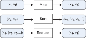
The responsibility of the user is to implement mappers and reducers — classes that extend Hadoop-provided base classes to solve a specific problem. As shown in Figure 3-1, a mapper takes input in a form of key/value pairs (k1, v1) and transforms them into another key/value pair (k2, v2). The MapReduce framework sorts a mapper’s output key/value pairs and combines each unique key with all its values (k2, {v2, v2,...}). These key/value combinations are delivered to reducers, which translate them into yet another key/value pair (k3, v3).
FIGURE 3-1: The functionality of mappers and reducers
A mapper and reducer together constitute a single Hadoop job. A mapper is a mandatory part of a job, and can produce zero or more key/value pairs (k2, v2). A reducer is an optional part of a job, and can produce zero or more key/value pairs (k3, v3). The user is also responsible for the implementation of a driver (that is, the main application controlling some of the aspects of the execution).
The responsibility of the MapReduce framework (based on the user-supplied code) is to provide the overall coordination of execution. This includes choosing appropriate machines (nodes) for running mappers; starting and monitoring the mapper’s execution; choosing appropriate locations for the reducer’s execution; sorting and shuffling output of mappers and delivering the output to reducer nodes; and starting and monitoring the reducer’s execution.
Now that you know what MapReduce is, let’s take a closer look at how exactly a MapReduce job is executed.
MapReduce Execution Pipeline
Any data stored in Hadoop (including HDFS and HBase) or even outside of Hadoop (for example, in a database) can be used as an input to the MapReduce job. Similarly, output of the job can be stored either in Hadoop (HDFS or HBase) or outside of it. The framework takes care of scheduling tasks, monitoring them, and re-executing failed tasks.
Figure 3-2 shows a high-level view of the MapReduce processing architecture.
FIGURE 3-2: High-level Hadoop execution architecture
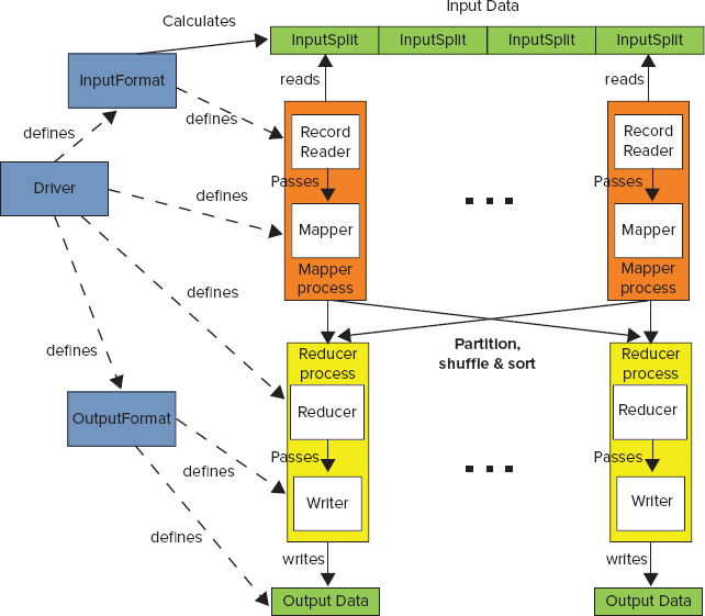
Following are the main components of the MapReduce execution pipeline:
- Driver — This is the main program that initializes a MapReduce job. It defines job-specific configuration, and specifies all of its components (including input and output formats, mapper and reducer, use of a combiner, use of a custom partitioner, and so on). The driver can also get back the status of the job execution.
- Context — The driver, mappers, and reducers are executed in different processes, typically on multiple machines. A context object (not shown in Figure 3-2) is available at any point of MapReduce execution. It provides a convenient mechanism for exchanging required system and job-wide information. Keep in mind that context coordination happens only when an appropriate phase (driver, map, reduce) of a MapReduce job starts. This means that, for example, values set by one mapper are not available in another mapper (even if another mapper starts after the first one completes), but is available in any reducer.
- Input data — This is where the data for a MapReduce task is initially stored. This data can reside in HDFS, HBase, or other storage. Typically, the input data is very large — tens of gigabytes or more.
- InputFormat — This defines how input data is read and split. InputFormat is a class that defines the InputSplits that break input data into tasks, and provides a factory for RecordReader objects that read the file. Several InputFormats are provided by Hadoop, and Chapter 4 provides examples of how to implement custom InputFormats. InputFormat is invoked directly by a job’s driver to decide (based on the InputSplits) the number and location of the map task execution.
- InputSplit — An InputSplit defines a unit of work for a single map task in a MapReduce program. A MapReduce program applied to a data set is made up of several (possibly several hundred) map tasks. The InputFormat (invoked directly by a job driver) defines the number of map tasks that make up the mapping phase. Each map task is given a single InputSplit to work on. After the InputSplits are calculated, the MapReduce framework starts the required number of mapper jobs in the desired locations.
- RecordReader — Although the InputSplit defines a data subset for a map task, it does not describe how to access the data. The RecordReader class actually reads the data from its source (inside a mapper task), converts it into key/value pairs suitable for processing by the mapper, and delivers them to the map method. The RecordReader class is defined by the InputFormat. Chapter 4 shows examples of how to implement a custom RecordReader.
- Mapper — The mapper performs the user-defined work of the first phase of the MapReduce program. From the implementation point of view, a mapper implementation takes input data in the form of a series of key/value pairs (k1, v1), which are used for individual map execution. The map typically transforms the input pair into an output pair (k2, v2), which is used as an input for shuffle and sort. A new instance of a mapper is instantiated in a separate JVM instance for each map task that makes up part of the total job input. The individual mappers are intentionally not provided with a mechanism to communicate with one another in any way. This allows the reliability of each map task to be governed solely by the reliability of the local machine.
- Partition — A subset of the intermediate key space (k2, v2) produced by each individual mapper is assigned to each reducer. These subsets (or partitions) are the inputs to the reduce tasks. Each map task may emit key/value pairs to any partition. All values for the same key are always reduced together, regardless of which mapper they originated from. As a result, all of the map nodes must agree on which reducer will process the different pieces of the intermediate data. The Partitioner class determines which reducer a given key/value pair will go to. The default Partitioner computes a hash value for the key, and assigns the partition based on this result. Chapter 4 provides examples on how to implement a custom Partitioner.
- Shuffle — Each node in a Hadoop cluster might execute several map tasks for a given job. Once at least one map function for a given node is completed, and the keys’ space is partitioned, the run time begins moving the intermediate outputs from the map tasks to where they are required by the reducers. This process of moving map outputs to the reducers is known as shuffling.
- Sort — Each reduce task is responsible for processing the values associated with several intermediate keys. The set of intermediate key/value pairs for a given reducer is automatically sorted by Hadoop to form keys/values (k2, {v2, v2,...}) before they are presented to the reducer.
- Reducer — A reducer is responsible for an execution of user-provided code for the second phase of job-specific work. For each key assigned to a given reducer, the reducer’s reduce() method is called once. This method receives a key, along with an iterator over all the values associated with the key. The values associated with a key are returned by the iterator in an undefined order. The reducer typically transforms the input key/value pairs into output pairs (k3, v3).
- OutputFormat — The way that job output (job output can be produced by reducer or mapper, if a reducer is not present) is written is governed by the OutputFormat. The responsibility of the OutputFormat is to define a location of the output data and RecordWriter used for storing the resulting data. Examples in Chapter 4 show how to implement a custom OutputFormat.
- RecordWriter — A RecordWriter defines how individual output records are written.
The following are two optional components of MapReduce execution (not shown in Figure 3-2):
- Combiner — This is an optional processing step that can be used for optimizing MapReduce job execution. If present, a combiner runs after the mapper and before the reducer. An instance of the Combiner class runs in every map task and some reduce tasks. The Combiner receives all data emitted by mapper instances as input, and tries to combine values with the same key, thus reducing the keys’ space, and decreasing the number of keys (not necessarily data) that must be sorted. The output from the Combiner is then sorted and sent to the reducers. Chapter 4 provides additional information about combiners.
- Distributed cache — An additional facility often used in MapReduce jobs is a distributed cache. This is a facility that enables the sharing of data globally by all nodes on the cluster. The distributed cache can be a shared library to be accessed by each task, a global lookup file holding key/value pairs, jar files (or archives) containing executable code, and so on. The cache copies over the file(s) to the machines where the actual execution occurs, and makes them available for the local usage. Chapter 4 provides examples that show how to use distributed cache for incorporating existing native code in the MapReduce execution.
One of the most important MapReduce features is the fact that it completely hides the complexity of managing a large distributed cluster of machines, and coordination of job execution between these nodes. A developer’s programming model is very simple — he or she is responsible only for implementation of mapper and reducer functionality, as well as a driver, bringing them together as a single job and configuring required parameters. All users’ code is then packaged into a single jar file (in reality, the MapReduce framework can operate on multiple jar files), that can be submitted for execution on the MapReduce cluster.
Runtime Coordination and Task Management in MapReduce
Once the job jar file is submitted to a cluster, the MapReduce framework takes care of everything else. It transparently handles all of the aspects of distributed code execution on clusters ranging from a single to a few thousand nodes.
The MapReduce framework provides the following support for application development:
- Scheduling — The framework ensures that multiple tasks from multiple jobs are executed on the cluster. Different schedulers provide different scheduling strategies ranging from “first come, first served,” to ensuring that all the jobs from all users get their fair share of a cluster’s execution. Another aspect of scheduling is speculative execution, which is an optimization that is implemented by MapReduce. If the JobTracker notices that one of the tasks is taking too long to execute, it can start an additional instance of the same task (using a different TaskTracker). The rationale behind speculative execution is ensuring that non-anticipated slowness of a given machine will not slow down execution of the task. Speculative execution is enabled by default, but you can disable it for mappers and reducers by setting the mapred.map.tasks.speculative.execution and mapred.reduce.tasks.speculative.execution job options to false, respectively.
- Synchronization — MapReduce execution requires synchronization between the map and reduce phases of processing. (The reduce phase cannot start until all of a map’s key/value pairs are emitted.) At this point, intermediate key/value pairs are grouped by key, which is accomplished by a large distributed sort involving all the nodes that executed map tasks, and all the nodes that will execute reduce tasks.
- Error and fault handling — To accomplish job execution in the environment where errors and faults are the norm, the JobTracker attempts to restart failed task executions. (You learn more about writing reliable MapReduce applications in Chapter 5.)
As shown in Figure 3-3, Hadoop MapReduce uses a very simple coordination mechanism. A job driver uses InputFormat to partition a map’s execution (based on data splits), and initiates a job client, which communicates with the JobTracker and submits the job for the execution. Once the job is submitted, the job client can poll the JobTracker waiting for the job completion. The JobTracker creates one map task for each split and a set of reducer tasks. (The number of created reduce tasks is determined by the job configuration.)
FIGURE 3-3: MapReduce execution
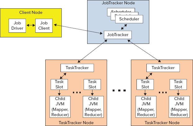
The actual execution of the tasks is controlled by TaskTrackers, which are present on every node of the cluster. TaskTrackers start map jobs and run a simple loop that periodically sends a heartbeat message to the JobTracker. Heartbeats have a dual function here — they tell the JobTracker that a TaskTracker is alive, and are used as a communication channel. As a part of the heartbeat, a TaskTracker indicates when it is ready to run a new task.
At this point, the JobTracker uses a scheduler to allocate a task for execution on a particular node, and sends its content to the TaskTracker by using the heartbeat return value. Hadoop comes with a range of schedulers (with fair scheduler currently being the most widely used one). Once the task is assigned to the TaskTracker, controlling its task slots (currently every node can run several map and reduce tasks, and has several map and reduce slots assigned to it), the next step is for it to run the task.
First, it localizes the job jar file by copying it to the TaskTracker’s filesystem. It also copies any files needed by the application to be on the local disk, and creates an instance of the task runner to run the task. The task runner launches from the distributed cache a new Java virtual machine (JVM) for task execution. The child process (task execution) communicates with its parent (TaskTracker) through the umbilical interface. This way, it informs the parent of the task’s progress every few seconds until the task is complete.
When the JobTracker receives a notification that the last task for a job is complete, it changes the status for the job to “completed.” The job client discovers job completion by periodically polling for the job’s status.
Now that you know what MapReduce is and its main components, you next look at how these components are used and interact during the execution of a specific application. The following section uses a word count example, which is functionally quite simple and is well explained in the MapReduce literature. This will preclude having to wade through any additional explanation, and will concentrate on the interaction between the application and the MapReduce pipeline.
YOUR FIRST MAPREDUCE APPLICATION
Listing 3-1 shows a very simple implementation of a word count MapReduce job.
LISTING 3-1: Hadoop word count implementation
import java.io.IOException;
import java.util.Iterator;
import java.util.StringTokenizer;

import org.apache.hadoop.conf.Configuration;
import org.apache.hadoop.conf.Configured;
import org.apache.hadoop.fs.Path;
import org.apache.hadoop.io.IntWritable;
import org.apache.hadoop.io.LongWritable;
import org.apache.hadoop.io.Text;
import org.apache.hadoop.mapreduce.Job;
import org.apache.hadoop.mapreduce.Mapper;
import org.apache.hadoop.mapreduce.Reducer;
import org.apache.hadoop.mapreduce.lib.input.TextInputFormat;
import org.apache.hadoop.mapreduce.lib.output.TextOutputFormat;
import org.apache.hadoop.util.Tool;
import org.apache.hadoop.util.ToolRunner;


public class WordCount extends Configured implements Tool{

     public static class Map extends Mapper<LongWritable, Text, Text,
       IntWritable> {
          private final static IntWritable one = new IntWritable(1);
          private Text word = new Text();
           @Override
          public void map(LongWritable key, Text value, Context context)
throws IOException, InterruptedException {
               String line = value.toString();
               StringTokenizer tokenizer = new StringTokenizer(line);
               while (tokenizer.hasMoreTokens()) {
                    word.set(tokenizer.nextToken());
                    context.write(word, one);
               }
          }
     }
     public static class Reduce extends Reducer<Text, IntWritable, Text,
       IntWritable>{
           @Override
           public void reduce(Text key, Iterable<IntWritable> val, Context
                context)
throws IOException, InterruptedException {
                int sum = 0;
                Iterator<IntWritable> values = val.iterator();
                while (values.hasNext()) {
                     sum += values.next().get();
                }
               context.write(key, new IntWritable(sum));
           }
     }

     public int run(String[] args) throws Exception {
          Configuration conf = new Configuration();
          Job job = new Job(conf, "Word Count");
          job.setJarByClass(WordCount.class);

          // Set up the input
          job.setInputFormatClass(TextInputFormat.class);
          TextInputFormat.addInputPath(job, new Path(args[0]));
          // Mapper
          job.setMapperClass(Map.class);
          // Reducer
          job.setReducerClass(Reduce.class);
          // Output
          job.setOutputFormatClass(TextOutputFormat.class);
          job.setOutputKeyClass(Text.class);
          job.setOutputValueClass(IntWritable.class);
          TextOutputFormat.setOutputPath(job, new Path(args[1]));
          //Execute
          boolean res = job.waitForCompletion(true);
          if (res)
               return 0;
          else
               return -1;
     }

     public static void main(String[] args) throws Exception {
          int res = ToolRunner.run(new WordCount(), args);
          System.exit(res);
     }
}This implementation has two inner classes — Map and Reduce — that extend Hadoop’s Mapper and Reducer classes, respectively.
The Mapper class has three key methods (which you can overwrite): setup, cleanup, and map (the only one that is implemented here). Both setup and cleanup methods are invoked only once during a specific mapper life cycle — at the beginning and end of mapper execution, respectively. The setup method is used to implement the mapper’s initialization (for example, reading shared resources, connecting to HBase tables, and so on), whereas cleanup is used for cleaning up the mapper’s resources and, optionally, if the mapper implements an associative array or counter, to write out the information.
The business functionality (that is, the application-specific logic) of the mapper is implemented in the map function. Typically, given a key/value pair, this method processes the pair and writes out (using a context object) one or more resulting key/value pairs. A context object passed to this method allows the map method to get additional information about the execution environment, and report on its execution. An important thing to note is that a map function does not read data. It is invoked (based on the “Hollywood principle”) every time a reader reads (and optionally parses) a new record with the data that is passed to it (through context) by the reader. If you are curious, take a look at the additional method (not widely advertised) in the base mapper class shown in Listing 3-2.
LISTING 3-2: Run method of the base mapper class
  /**
   * Expert users can override this method for more complete control over the
   * execution of the Mapper.
   * @param context
   * @throws IOException
   */
  public void run(Context context) throws IOException, InterruptedException {
    setup(context);
    while (context.nextKeyValue()) {
      map(context.getCurrentKey(), context.getCurrentValue(), context);
    }
    cleanup(context);
  }
This is the method behind most of the magic of the mapper class execution. The MapReduce pipeline first sets up execution — that is, does all necessary initialization (see, for example, Chapter 4 for a description of RecordReader initialization). Then, while input records exist for this mapper, the map method is invoked with a key and value passed to it. Once all the input records are processed, a cleanup is invoked, including invocation of cleanup method of the mapper class itself.
Similar to mapper, a reducer class has three key methods — setup, cleanup, and reduce — as well as a run method (similar to the run method of the mapper class shown in Listing 3-2). Functionally, the methods of the reducer class are similar to the methods of the mapper class. The difference is that, unlike a map method that is invoked with a single key/value pair, a reduce method is invoked with a single key and an iterable set of values (remember, a reducer is invoked after execution of shuffle and sort, at which point, all the input key/value pairs are sorted, and all the values for the same key are partitioned to a single reducer and come together). A typical implementation of the reduce method iterates over a set of values, transforms all the key/value pairs in the new ones, and writes them to the output.
The WordCount class itself implements the Tool interface, which means that it must implement the run method responsible for configuring the MapReduce job. This method first creates a configuration object, which is used to create a job object.
A default configuration object constructor (used in the example code) simply reads the default configuration of the cluster. If some specific configuration is required, it is possible to either overwrite the defaults (once configuration is created), or set additional configuration resources that are used by a configuration constructor to define additional parameters.
A job object represents job submitter’s view of the job. It allows the user to configure the job’s parameters (they will be stored in the configuration object), submit it, control its execution, and query its state.
Job setup is comprised of the following main sections:
- Input setup — This is set up as InputFormat, which is responsible for calculation of the job’s input split and creation of the data reader. In this example, TextInputFormat is used. This InputFormat leverages its base class (FileInputFormat) to calculate splits (by default, this will be HDFS blocks) and creates a LineRecordReader as its reader. Several additional InputFormats supporting HDFS, HBase, and even databases are provided by Hadoop, covering the majority of scenarios used by MapReduce jobs. Because an InputFormat based on the HDFS file is used in this case, it is necessary to specify the location of the input data. You do this by adding an input path to the TextInputFormat class. It is possible to add multiple paths to the HDFS-based input format, where every path can specify either a specific file or a directory. In the latter case, all files in the directory are included as an input to the job.
- Mapper setup — This sets up a mapper class that is used by the job.
- Reducer setup — This sets up reducer class that is used by the job. In addition, you can set up the number of reducers that are used by the job. (There is a certain asymmetry in Hadoop setup. The number of mappers depends on the size of the input data and split, whereas the number of reducers is explicitly settable.) If this value is not set up, a job uses a single reducer. For MapReduce applications that specifically do not want to use reducers, the number of reducers must be set to 0.
- Output setup — This sets up output format, which is responsible for outputting results of the execution. The main function of this class is to create an OutputWriter. In this case, TextOutputFormat (which creates a LineRecordWriter for outputting data) is used. Several additional OutputFormats supporting HDFS, HBase, and even databases are provided with Hadoop, covering the majority of scenarios used by MapReduce jobs. In addition to the output format, it is necessary to specify data types used for output of key/value pairs (Text and IntWritable, in this case), and the output directory (used by the output writer). Hadoop also defines a special output format — NullOutputFormat — which should be used in the case where a job does not use an output (for example, it writes its output to HBase directly from either map or reduce). In this case, you should also use NullWritable class for output of key/value pair types.
Finally, when the job object is configured, a job can be submitted for execution. Two main APIs are used for submitting a job using a Job object:
- The submit method submits a job for execution, and returns immediately. In this case, if, at some point, execution must be synchronized with completion of the job, you can use a method isComplete() on a Job object to check whether the job has completed. Additionally, you can use the isSuccessful() method on a Job object to check whether a job has completed successfully.
- The waitForCompletion method submits a job, monitors its execution, and returns only when the job is completed.
Hadoop development is essentially Java development, so you should use your favorite Java IDE. Eclipse usage for Hadoop development is discussed here.
Building and Executing MapReduce Programs
Using Eclipse for developing Hadoop code is really straightforward. Assuming that your instance of Eclipse is configured with Maven, first create a Maven project for your implementation. Because there is no Hadoop Maven archetype, start with the “simple” Maven project and add pom.xml manually, similar to what is shown in Listing 3-3.
LISTING 3-3: pom.xml for Hadoop 2.0
<project xmlns="http://maven.apache.org/POM/4.0.0"
          xmlns:xsi="http://www.w3.org/2001/XMLSchema-instance"
     xsi:schemaLocation="http://maven.apache.org/POM/4.0.0
          http://maven.apache.org/xsd/maven-4.0.0.xsd">
     <modelVersion>4.0.0</modelVersion>
     <groupId>com.nokia.lib</groupId>
     <artifactId>nokia-cgnr-sparse</artifactId>
     <version>0.0.1-SNAPSHOT</version>
     <name>cgnr-sparse</name>
     <properties>
          <hadoop.version>2.0.0-mr1-cdh4.1.0</hadoop.version>
          <hadoop.common.version>2.0.0-cdh4.1.0</hadoop.common.version>
          <hbase.version>0.92.1-cdh4.1.0</hbase.version>
     </properties>
     <repositories>
          <repository>
               <id>CDH Releases and RCs Repositories</id>
               <url>https://repository.cloudera.com/content/groups/cdh-
                    releases-rcs</url>
          </repository>
     </repositories>
     <build>
          <plugins>
               <plugin>
                    <groupId>org.apache.maven.plugins</groupId>
                    <artifactId>maven-compiler-plugin</artifactId>
                    <version>2.3.2</version>
                    <configuration>
                         <source>1.6</source>
                         <target>1.6</target>
                    </configuration>
               </plugin>
          </plugins>
     </build>
     <dependencies>
          <dependency>
               <groupId>org.apache.hadoop</groupId>
               <artifactId>hadoop-core</artifactId>
               <version>${hadoop.version}</version>
               <scope>provided</scope>
          </dependency>
          <dependency>
               <groupId>org.apache.hbase</groupId>
               <artifactId>hbase</artifactId>
               <version>${hbase.version}</version>
               <scope>provided</scope>
          </dependency>
          <dependency>
               <groupId>org.apache.hadoop</groupId>
               <artifactId>hadoop-common</artifactId>
               <version>${hadoop.common.version}</version>
               <scope>provided</scope>
          </dependency>
          <dependency>
               <groupId>junit</groupId>
               <artifactId>junit</artifactId>
               <version>4.10</version>
          </dependency>
     </dependencies>
</project>The pom file shown in Listing 3-3 is for Cloudera CDH 4.1 (note the inclusion of the Cloudera repository in the pom file). It includes a minimal set of dependencies necessary for developing a Hadoop MapReduce job — hadoop-core and hadoop-common. Additionally, if you use HBase for an application, you should include an hbase dependency. It also contains junit for supporting basic unit tests. Also note that all Hadoop-related dependences are specified as provided. This means that they will not be included in the final jar file generated by Maven.
Once the Eclipse Maven project is created, all of the code for your MapReduce implementation goes into this project. Eclipse takes care of loading required libraries, compiling your Java code, and so on.
Now that you know how to write a MapReduce job, take a look at how to execute it. You can use the Maven install command to generate a jar file containing all the required code. Once a jar file is created, you can FTP it to the cluster’s edge node, and executed using the command shown in Listing 3-4.
LISTING 3-4: Hadoop execution command
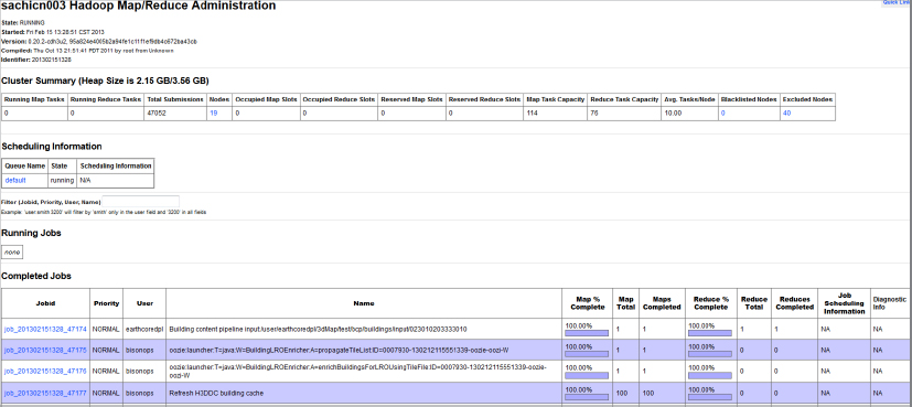
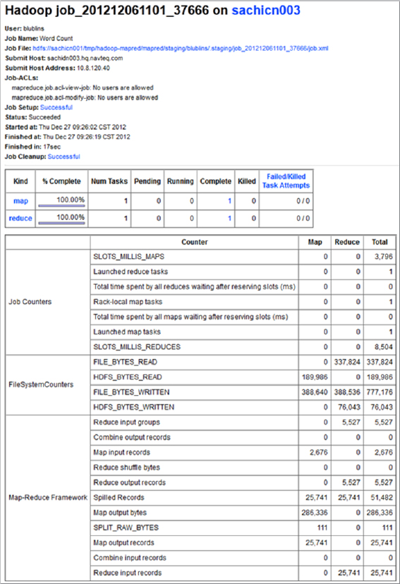
hadoop jar your.jar mainClass inputpath outputpathHadoop provides several JavaServer Pages (JSPs), enabling you to visualize MapReduce execution. The MapReduce administration JSP enables you to view both the overall state of the cluster and details of the particular job execution. The MapReduce administration main page shown in Figure 3-4 displays the overall state of the cluster, as well as a list of currently running, completed, and failed jobs. Every job in every list (running, completed, and failed) is “clickable,” which enables you to get additional information about job execution.
FIGURE 3-4: MapReduce administration main page
The job detail page shown in Figure 3-5 provides (dynamic) information about execution. The page exists starting from the point when the JobTracker accepts the job, and keeps track of all the changes during the job execution. You can also use it for post-mortem analysis of the job execution. This page has the following four main parts (with the fourth one not shown on Figure 3-5):
- The first part (top of the page) displays the combined information about the job, including job name, user, submitting host, start and end time, execution time, and so on.
- The second part contains summary information about mappers/reducers for a given job. It tells how many mappers and reducers a job has, and splits them by their states — pending, running, complete, and killed.
- The third part show jobs counters (for an in-depth discussion on counters, see Chapter 4), which are split by namespaces. Because this example implementation does not use custom counters, only standard ones appear for it.
- The fourth part provides nice histograms detailing mapper and reducer execution.
FIGURE 3-5: WordCount job page
The job detail page provides more information (through the “clickable links”), which helps you to analyze job execution further. Those pages are discussed in detail in Chapter 5 during a discussion about building reliable MapReduce applications.
Next, you look at the design of MapReduce applications.
DESIGNING MAPREDUCE IMPLEMENTATIONS
As discussed, the power of MapReduce comes from its simplicity. In addition to preparing the input data, the programmer must only implement the mapper and reducer. Many real-life problems can be solved using this approach.
In the most general case, MapReduce can be thought of as a general-purpose parallel execution framework that can take full advantage of the data locality. But this simplicity comes with a price — a designer must decide how to express his or her business problem in terms of a small number of components that must fit together in very specific ways.
To reformulate the initial problem in terms of MapReduce, it is typically necessary to answer the following questions:
- How do you break up a large problem into smaller tasks? More specifically, how do you decompose the problem so that the smaller tasks can be executed in parallel?
- Which key/value pairs can you use as inputs/outputs of every task?
- How do you bring together all the data required for calculation? More specifically, how do you organize processing the way that all the data necessary for calculation is in memory at the same time?
It is important to realize that many algorithms cannot be easily expressed as a single MapReduce job. It is often necessary to decompose complex algorithms into a sequence of jobs, where data output of one job becomes the input to the next.
This section takes a look at several examples of designing MapReduce applications for different practical problems (from very simple to more complex). All of the examples are described in the same format:
- A short description of the problem
- A description of the MapReduce job(s), including the following:
- Mapper description
- Reducer description
Using MapReduce as a Framework for Parallel Processing
In the simplest case, source data is organized as a set of independent records, and the results can be specified in any order. These classes of problems (“embarrassing parallel” problems) require the same processing to be applied to each data element in a fairly independent way — in other words, there is no need to consolidate or aggregate individual results. A classic example would be processing several thousand PDF files to extract some key text and place into a CSV file for later insertion into a database.
Implementation of MapReduce in this situation is very simple — the only thing that is required is the mapper, processing each record independently and outputting the result. In this case, MapReduce controls distribution of the mappers, and provides all of the support required for scheduling and error handling. The following example shows how to design this type of application.
Face Recognition Example
Although not often discussed as a Hadoop-related problem, an image-processing implementation fits really well in the MapReduce paradigm. Assume that there is a face-recognition algorithm implementation that takes an image, recognizes a set of desired features, and produces a set of recognition results. Also assume that it is necessary to run face recognition on millions of pictures.
If all the pictures are stored in Hadoop in the form of a sequence file, then you can use a simple map-only job to parallelize execution. A set of input key/value pairs in this case is imageID/Image, and a set of output key/value pairs is imageID/list of recognized features. Additionally, a set of recognizable features must be distributed to all mappers (for example, using the distributed cache).
Table 3-1 shows the implementation of a MapReduce job for this example.
TABLE 3-1: Face Recognition Job
| PROCESS PHASE | DESCRIPTION |
| Mapper | In this job, a mapper is first initialized with the set of recognizable features. For every image, a map function invokes a face-recognition algorithm implementation, passing it an image itself, along with a list of recognizable features. The result of recognition, along with the original imageID, is output from the map. |
| Result | A result of this job execution is recognition of all the images contained in the original images. |
Now take a look at a more complex case, where the results of the map execution must be grouped together (that is, ordered in certain way). Many practical implementations (including filtering, parsing, data conversion, summing, and so on) can be solved with this type of a MapReduce job.
Simple Data Processing with MapReduce
An example of such a case is the building of inverted indexes. These types of problems require a full MapReduce implementation where shuffle and sort are required to bring all results together. The following example shows how to design this type of application.
Inverted Indexes Example
In computer science, an inverted index is a data structure that stores a mapping from content (such as words or numbers) to its location in a document or a set of documents, as shown in Figure 3-6. The purpose of an inverted index is to allow fast full-text searches, at a cost of increased processing during a document addition. The inverted index data structure is a central component of a typical search engine, enabling you to optimize the speed of finding the documents in which a certain word occurs.
FIGURE 3-6: Inverted index
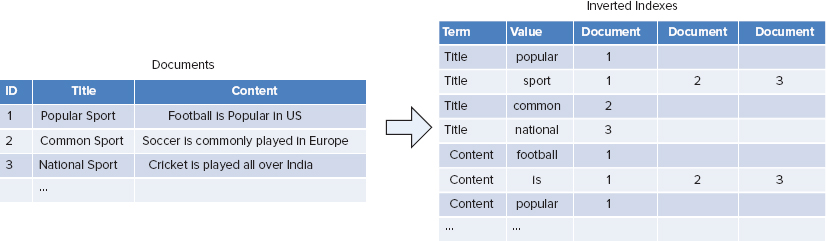
To build an inverted index, it is possible to feed the mapper each document (or lines within a document). The mapper will parse the words in the document to emit [word, descriptor] pairs. The reducer can simply be an identity function that just writes out the list, or it can perform some statistic aggregation per word.
Table 3-2 shows the implementation of a MapReduce job for this example.
TABLE 3-2: Calculation of Inverted Indexes Job
| PROCESS PHASE | DESCRIPTION |
| Mapper | In this job, the role of the mapper is to build a unique record containing a word index, and information describing the word occurrence in the document. It reads every input document, parses it, and, for every unique word in the document, builds an index descriptor. This descriptor contains a document ID, number of times the index occurs in the document, and any additional information (for example, index positions as offset from the beginning of the document). Every index descriptor pair is written out. |
| Shuffle and Sort | MapReduce’s shuffle and sort will sort all the records based on the index value, which guarantees that a reducer will get all the indexes with a given key together. |
| Reducer | In this job, the role of a reducer is to build an inverted indexes structure. Depending on the system requirements, there can be one or more reducers. A reducer gets all the descriptors for a given index, and builds an index record, which is written to the desired index storage. |
| Result | A result of this job execution is an inverted index for a set of the original documents. |
More complex MapReduce applications require bringing data from the multiple sources (in other words, joining data) for processing. Next you look at how to design, implement, and use data joins using MapReduce.
Building Joins with MapReduce
A generic join problem can be described as follows. Given multiple data sets (S1 through Sn), sharing the same key (a join key), you want to build records containing a key and all required data from every record.
Two “standard” implementations exist for joining data in MapReduce: reduce-side join and map-side join.
A most common implementation of a join is a reduce-side join. In this case, all data sets are processed by the mapper that emits a join key as the intermediate key, and the value as the intermediate record capable of holding either of the set’s values. Because MapReduce guarantees that all values with the same key are brought together, all intermediate records will be grouped by the join key, which is exactly what is necessary to perform the join operation. This works very well in the case of one-to-one joins, where at most one record from every data set has the same key.
Although theoretically this approach will also work in the case of one-to-many and many-to-many joins, these cases can have additional complications. When processing each key in the reducer, there can be an arbitrary number of records with the join key. The obvious solution is to buffer all values in memory, but this can create a scalability bottleneck, because there might not be enough memory to hold all the records with the same join key. This situation typically requires a secondary sort, which can be achieved with the value-to-key conversion design pattern.
for every product p:
for every purchase (p, s):
sum(productInfo.price * purchaseInfo.quantity)The following example shows how you can use reduce-side joins in a realistic application.
Road Enrichment Example
The heart of a road enrichment algorithm is joining a nodes data set (containing a node ID and some additional information about the node) with a link data set (containing link ID, IDs of the nodes that link connects, and some additional information about the link, including the number of link lanes) based on the node IDs.
A simplified road enrichment algorithm that leverages a reduce-side join might include the following steps:
FIGURE 3-7: Road enrichment
For the implementation of this algorithm, assume the following:
- A node is described with an object N with the key NN1 ... NNm. For example, node N1 can be described as NN1 and N2 as NN2. All nodes are stored in the nodes input file.
- A link is described with an object L with the key LL1 ... LLm. For example, link L1 can be described as LL1, L2 as LL2, and so on. All the links are stored in the links source file.
- Also introduce an object of the type link or node (LN), which can have any key.
- Finally, it is necessary to define two more types — intersection (S) and road (R).
With this in place, a MapReduce implementation for the road enrichment can consist of two MapReduce jobs.
Table 3-3 shows the implementation of the first MapReduce job for this example.
TABLE 3-3: Calculation of Intersection Geometry and Moving the Road’s End Points Job
| PROCESS PHASE | DESCRIPTION |
| Mapper | In this job, the role of the mapper is to build LNNi records out of the source records — NNi and LLi. It reads every input record from both source files, and then looks at the object type. If it is a node with the key NNi, a new record of the type LNNi is written to the output. If it is a link, keys of both adjacent nodes (NNi and NNj) are extracted from the link and two records (LNNi and LNNj) are written out. |
| Shuffle and Sort | MapReduce’s shuffle and sort will sort all the records based on the node’s keys, which guarantees that every node with all adjacent links will be processed by a single reducer, and that a reducer will get all the LN records for a given key together. |
| Reducer | In this job, the role of the reducer is to calculate intersection geometry and move the road’s ends. It gets all LN records for a given node key and stores them in memory. Once all of them are in memory, the intersection’s geometry can be calculated and written out as an intersection record with node key SNi. At the same time, all the link records connected to a given node can be converted to road records and written out with a link key — RLi. |
| Result | A result of this job execution is a set of intersection records ready to use, and road records that must be merged together. (Every road is connected to two intersections, and dead ends are typically modeled with a node that has a single link connected to it.) It is necessary to implement the second MapReduce job to merge them. (By default, the output of the MapReduce job writes out the mixture of roads and intersections, which is not ideal. For the purposes here, you would like to separate intersections that are completed, and roads that require additional processing into different files. Chapter 4 examines the way to implement a multi-output format.) |
Table 3-4 shows implementation of the second MapReduce job for this example.
TABLE 3-4: Merge Roads Job
| PROCESS PHASE | DESCRIPTION |
| Mapper | The role of the mapper in this job is very simple. It is just a pass-through (or identity mapper in Hadoop’s terminology). It reads road records and writes them directly to the output. |
| Shuffle and Sort | MapReduce’s shuffle and sort will sort all the records based on the link’s keys, which guarantees that both road records with the same key will come to the same reducer together. |
| Reducer | In this job, the role of the reducer is to merge roads with the same ID. Once the reducer reads both records for a given road, it merges them together, and writes them out as a single road record. |
| Result | A result of this job execution is a set of road records ready to use. |
Now take a look at a special case of a reducer join called a “Bucketing” join. In this case, the data sets might not have common keys, but support the notion of proximity (for example, geographic proximity). In this case, a proximity value can be used as a join key for the data sets. A typical example would be geospatial processing based on the bounding box discussed in the following example.
Links Elevation Example
This problem can be defined as follows. Given a links graph and terrain model, convert two-dimensional (x,y) links into three-dimensional (x, y, z) links. This process is called link elevation.
Assume the following:
- Every link is specified as two connected points — start and end.
- A terrain model is stored in HBase. (Although HDFS has been used in the examples so far, all of the approaches described earlier are relevant to the HBase-stored data as well. There is one serious limitation, though. The current table input format is limited to processing one table. You learn how to implement a table join in Chapter 4.) The model is stored in the form of a height’s grids for tiles keyed by the tile ID. (Tiling is a partitioning of a space — the whole world in this case — into a finite number of distinct shapes. Here, equal-sized bounding boxes are used as tiles.)
Figure 3-8 shows the model.
FIGURE 3-8: Mapping roads to tiles
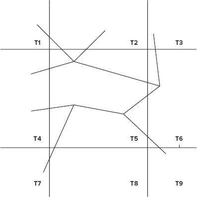
A simplified link elevation algorithm is based on “bucketing” links into tiles, then joining every link’s tile with the elevation tile, and processing the complete tile containing both links and elevation data. The algorithm looks as follows:
The actual implementation consists of two MapReduce jobs. Table 3-5 shows the implementation of the first MapReduce job for this example.
TABLE 3-5: Split Links into Pieces and Elevate Each Piece Job
| PROCESS PHASE | DESCRIPTION |
| Mapper | In this job, the role of the mapper is to build link pieces, and assign them to the individual tiles. It reads every link record, and splits them into fixed-length fragments, which effectively converts link representation into a set of points. For every point, it calculates a tile to which this point belongs, and produces one or more link piece records, which may be represented as (tid, {lid [points array]}), where tid is tile ID, lid is the original link ID, and points array is an array of points from the original link, which belong to a given tile. |
| Shuffle and Sort | MapReduce’s shuffle and sort will sort all the records based on the tile’s IDs, which guarantees that all of the link’s pieces belonging to the same tile will be processed by a single reducer. |
| Reducer | In this job, the role of the reducer is to calculate elevation for every link piece. For every tile ID, it loads terrain information for a given tile from HBase, and then reads all of the link pieces and calculates elevation for every point. It outputs the record (lid, [points array]), where lid is original link ID and points array is an array of three-dimensional points. |
| Result | A result of this job execution contains fully elevated link pieces. It is necessary to implement the second MapReduce job to merge them. |
Table 3-6 shows the implementation of the second MapReduce job for this example.
TABLE 3-6: Combine Link’s Pieces into Original Links Job
| PROCESS PHASE | DESCRIPTION |
| Mapper | The role of the mapper in this job is very simple. It is an identity mapper. It reads link piece records and writes them directly to the output in the form of (lid, [points array]) key/value pairs. |
| Shuffle and Sort | MapReduce’s shuffle and sort will sort all the records based on the link’s keys, which guarantees that all link piece records with the same key will come to the same reducer together. |
| Reducer | In this job, the role of the reducer is to merge link pieces with the same ID. Once the reducer reads all of them, it merges them together, and writes them out as a single link record. |
| Result | A result of this job execution contains elevated links ready to use. |
Despite the power of the reducer-side join, its execution can be fairly expensive — shuffle and sort of the large data sets can be very resource-intensive. In the cases when one of the data sets is small enough (“baby” joins) to fit in memory, a map in memory side join can be used. In this case, a small data set is brought into memory in a form of key-based hash providing fast lookups. Now it is possible to iterate over the larger data set, do all the joins in memory, and output the resulting records.
For such an implementation to work, a smaller data set must be distributed to all of the machines where mappers are running. Although it is simple enough to put a smaller data set into HDFS and read it on the mapper startup, Hadoop provides a better solution for this problem — a distributed cache. The native code integration discussion in Chapter 4 provides more details on using the distributed cache.
Problems discussed so far have required implementation of a predefined number of MapReduce jobs. Many practical algorithms (for example, graph processing, or mathematical calculations) are iterative in nature, requiring repeated execution until some convergence criteria is met. Next you look at how to design iterative MapReduce applications.
Building Iterative MapReduce Applications
In the case of iterative MapReduce applications, one or more MapReduce jobs are typically implemented in the loop. This means that such applications can either be implemented using a driver that internally implements an iteration logic and invokes a required MapReduce job(s) inside such an iteration loop, or an external script running MapReduce jobs in a loop and checking conversion criteria. (Another option is using a workflow engine. Chapters 6 through 8 examine Hadoop’s workflow engine called Apache Oozie.) Using a driver for execution of iterative logic often provides a more flexible solution, enabling you to leverage both internal variables and the full power of Java for implementation of both iterations and conversion checks.
A typical example of an iterative algorithm is solving a system of linear equations. Next you look at how you can use MapReduce for designing such an algorithm.
Solving Linear Equations Example
Numerous practical problems can be expressed in terms of solving a system of linear equations, or at least reduced to such a system. Following are some examples:
- Optimization problems that can be solved with linear programming
- Approximation problems (for example, polynomial splines)
Solving linear equations efficiently when the size of the problem is significant — in the ballpark of hundreds of thousands of variables or higher — can be challenging. In this case, the alternative is either to use supercomputers with terabytes of memory, or use the algorithms that allow piecemeal computations and do not require the complete matrix to be brought in memory. The classes of algorithms that adhere to these requirements are iterative methods that provide approximate solutions, with performance tied to the number of iterations necessary to find a solution within a required precision.
With these types of algorithms, the conjugate gradient (CG) method offers the best performance when the system matrix is right. Following is the basic equation in the system of linear equations:
Ax = b
With CG, you can implement the method of steepest descent applied to the quadratic surface in Rn defined as follows:
f(x) = 1/2xTAx − xTb, x![]() Rn
Rn
Each step improves the solution vector in the direction of the extreme point. Each step’s increment is a vector conjugate with respect to A to all vectors found in previous steps.
The CG algorithm includes the following steps:
The solution is xk+1.
The only “expensive” operation in this algorithm implementation is the calculation of residual vector (found in steps 2 and 4c), which requires matrix vector multiplication. This operation can be easily implemented using MapReduce.
Assume you have two HBase tables — one for matrix A and one for all the vectors. If matrix A is sparse, then a reasonable HBase data layout is as follows:
- Each table row represents a single matrix row.
- All elements of a given matrix row are stored in a single column family with a column name corresponding to a column of a given matrix element, and a value corresponding to a matrix value in this row, column value. Considering that the matrix is sparse, the number of columns is going to be significantly smaller than the number of rows.
Although explicit columns for matrix columns are not required for vector multiplication implementation, this table layout might be handy if it is necessary to set/update individual matrix elements.
A reasonable HBase data layout for representing vectors is as follows:
- Each table row represents a single vector.
- All elements of a given vector are stored in a single column family, with a column name corresponding to a vector index, and a value corresponding to a vector value for an index.
Although, technically, it is possible to use different tables for different vectors using vector indexes as row keys, the proposed layout makes reading/writing vectors significantly faster (single-row reads/writes) and minimizes the amount of HBase connections opened at the same time.
With the HBase table’s design in place, a MapReduce matrix vector implementation is fairly straightforward. A single mapper will do the job. Table 3-7 shows the implementation of the matrix vector multiplication MapReduce job.
TABLE 3-7: Matrix Vector Multiplication Job
| PROCESS PHASE | DESCRIPTION |
| Mapper | In this job, a mapper is first initialized with the value of a vector. For every row of the matrix (r), vector multiplication of the source vector and matrix row is calculated. The resulting value (nonzero) is stored at index r of the resulting vector. |
In this implementation, the MapReduce driver executes the algorithm described previously, invoking the matrix vector multiplication MapReduce job every time multiplication is required.
Although the algorithm described here is fairly simple and straightforward to implement, in order for CG to work, the following conditions must be met:
- Matrix A must be definite-positive. This provides for a convex surface with a single extreme point. It means that the method will converge with any choice of the initial vector x0.
- Matrix A must be symmetric. This ensures the existence of an A-orthogonal vector at each step of the process.
If matrix A is not symmetric, it can be made symmetric by replacing the initial equation with the following one:
ATAx = ATb
ATA is symmetric and positive. As a result, the previously described algorithm can be applied as is. In this case, the implementation of the original algorithm carries significant performance penalties of calculating the new system matrix ATA. Additionally, convergence of the method will suffer, because k(ATA) = k(A)2.
Fortunately, you have the choice of not computing ATA up front, and instead modifying the previous algorithm’s steps 2, 4a, and 4c, as shown here:
- Step 2 — To compute ATAx0, perform two matrix vector multiplications: AT(Ax0).
- Step 4a — To compute the denominator pkTATApk, note that it is equal to (Apk)2, and its computation comes down to a matrix vector multiplication and an inner product of the result with itself.
- Step 4c — Similar to step 2, perform two matrix vector multiplications: AT(Apk).
So, the overall algorithm implementation first must check whether matrix A is symmetric. If it is, then the original algorithm is used; otherwise, the modified algorithm is used.
In addition to the first job, implementation of the overall algorithm requires one more MapReduce job — matrix transposition. Table 3-8 shows the implementation of the matrix transposition MapReduce job.
TABLE 3-8: Matrix Transposition Job
| PROCESS PHASE | DESCRIPTION |
| Mapper | In this job, for every row of matrix (r), each element (r, j) is written to the result matrix as element (j, r). |
Note that, in this example, an algorithm conversion criterion is an integral part of the algorithm calculation itself. In the next example, the conversion criterion calculation uses a Hadoop-specific technique.
Stranding Bivalent Links Example
A fairly common mapping problem is stranding bivalent links.
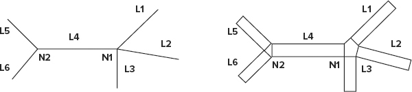
Two connected links are called bivalent if they are connected via a bivalent node. A bivalent node is a node that has only two connections. For example, in Figure 3-9, nodes N6, N7, N8, and N9 are bivalent. Links L5, L6, L7, L8, and L9 are also bivalent. A degenerate case of a bivalent link is link L4.
FIGURE 3-9: Example of bivalent links
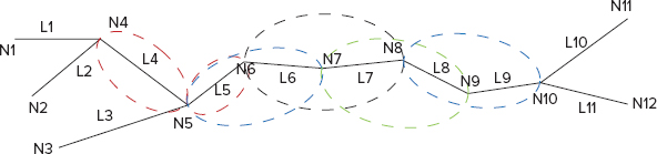
As shown in Figure 3-9, an algorithm for calculating bivalent link stretches looks very straightforward — any stretch of links between two non-bivalent nodes is a stretch of bivalent links.
For implementation of this algorithm, assume the following:
- A node is described with an object N with the key Ni - NNi. For example, node N1 can be described as NN1 and N2 as NN2.
- A link is described with an object L with the key Li – LLi. For example, link L1 can be described as LL1, L2 as LL2, and so on. A link object contains references to its start and end nodes (NNi, NNj).
- Also introduce an object of the type link(s) or node (LN), which can have any key, and can contain either node or one or more links.
- Finally, define one more type — a link’s strand (S). This data type contains a linked list of links in the strand.
With this in place, an algorithm for stranding of bivalent links looks as follows:
The actual implementation consists of two MapReduce jobs. The first one prepares the initial strands, and the second one (executed in the loop) combines partial strands. In this case, the actual combining of the strands is done as part of the MapReduce job execution. As a result, those jobs (not the driver) know how many partial strands were combined during execution. Fortunately, Hadoop provides a simple mechanism for communicating between a driver and MapReduce execution — counters.
Table 3-9 shows the implementation of the first MapReduce job for this example.
TABLE 3-9: Elimination of Non-Bivalent Nodes Job
| PROCESS PHASE | DESCRIPTION |
| Mapper | In this job, the role of the mapper is to build LNNi records out of the source records — NNi and LLi. It reads every input record, and then looks at the object type. If it is a node with the key Ni, a new record of the type LNNi is written to the output. If it is a link, keys of the both adjacent nodes (Ni and Nj) are extracted from the link, and two records (LNNi and LNNj ) are written out. |
| Shuffle and Sort | MapReduce’s shuffle and sort will sort all the records based on the node’s keys, which guarantees that every node with all adjacent links will be processed by a single reducer, and that a reducer will get all the LN records for a given key together. |
| Reducer | In this job, the role of the reducer is to eliminate non-bivalent nodes and build partial link strands. It reads all LN records for a given node key and stores them in memory. If the number of links for this node is 2, then this is a bivalent node, and a new strand (combining these two nodes) is written to the output (for example, see pairs L5, L6 or L7, L8). If the number of links is not equal to 2 (it can be either a dead-end or a node at which multiple links intersect), then this is a non-bivalent node. For this type of node, a special strand is created containing a single link, connected to this non-bivalent node (for example, see L4 or L5). The number of strands for such node is equal to the number of links connected to this node. |
| Result | A result of this job execution contains partial strand records, some of which can be repeated (L4, for example, will appear twice — from processing N4 and N5). |
Table 3-10 shows the implementation of the second MapReduce job for this example.
TABLE 3-10: Merging Partial Strands Job
| PROCESS PHASE | DESCRIPTION |
| Mapper | The role of the mapper in this job is to bring together strands sharing the same links. For every strand it reads, it outputs several key/value pairs. The key values are the keys of the links in the strand, and the values are the strands themselves. |
| Shuffle and Sort | MapReduce’s shuffle and sort will sort all the records based on end link keys, which guarantees that all strand records containing the same link ID will come to the same reducer together. |
| Reducer |
|
| Result | A result of this job execution contains all complete strands in a separate directory. It also contains a directory of all bivalent partial strands, along with the value of the “to be processed” counter. |
The examples presented here just start to scratch the surface of potential MapReduce usage for solving real-world problems. Next you take a closer look at the situations where MapReduce usage is appropriate, and where it is not.
To MapReduce or Not to MapReduce?
As discussed, MapReduce is a technique used to solve a relatively simple problem in situations where there is a lot of data, and it must be processed in parallel (preferably on multiple machines). The whole idea of the concept is that it makes it possible to do calculations on massive data sets in a realistic time frame.
Alternatively, MapReduce can be used for parallelizing compute-intensive calculations, where it’s not necessarily about the amount of data, but rather about the overall calculation time (typically the case of “embarrassingly parallel” computations).
The following must be true in order for MapReduce to be applicable:
- The calculations that need to be run must be composable. This means that you should be able run the calculation on a subset of data, and merge partial results.
- The data set size is big enough (or the calculations are long enough) that the infrastructure overhead of splitting it up for independent computations and merging results will not hurt overall performance.
- The calculation depends mostly on the data set being processed. Additional small data sets can be added using HBase, distributed cache, or some other techniques.
MapReduce is not applicable, however, in scenarios when the data set must be accessed randomly to perform the operation (for example, if a given data set record must be combined with additional records to perform the operation). However, in this case, it is sometimes possible to run additional MapReduce jobs to “prepare” data for calculations.
Another set of problems that are not applicable for MapReduce are recursive problems (for example, a Fibonacci problem). MapReduce is not applicable in this case because computation of the current value requires the knowledge of the previous one. This means that you can’t break it apart into sub-computations that can be run independently.
If a data size is small enough to fit in a single machine’s memory, it is probably going to be faster to process it as a standalone application. Usage of MapReduce, in this case, makes implementation unnecessarily complex and typically slower.
Keep it in mind that, although it is true that a large class of algorithms is not directly applicable to MapReduce implementations, there often exist alternative solutions to the same underlying problems that can be solved by leveraging MapReduce. In this case, usage of MapReduce is typically advantageous, because of the richness of the Hadoop ecosystem in which MapReduce is executed (which supports easier enhancements to the implementation, and integration with other applications).
Finally, you should remember that MapReduce is inherently a batch implementation and should never be used for online computations (for example, real-time calculations for online users’ requests).
Common MapReduce Design Gotchas
Following is a list of some things to watch for and avoid when you design your MapReduce implementation:
- When splitting data between map tasks, ensure that you do not create too many (typically, the number of mappers should be in hundreds, not thousands) or too few of them. Having the right number of maps has the following advantages for applications:
- Having too many mappers creates scheduling and infrastructure overhead, and, in extreme cases, can even kill a JobTracker. Also, having too many mappers typically increases overall resource utilization (because of the creation of excessive JVMs) and execution time (because of the limited number of execution slots).
- Having too few mappers can lead to underutilization of the cluster, and the creation of too much load on some of the nodes (where maps actually run). Additionally, in the case of very large map tasks, retries and speculative execution becomes very expensive and takes longer.
- A large number of small mappers creates a lot of seeks during shuffle of the map output to the reducers. It also creates too many connections delivering map outputs to the reducers.
- The number of reducers configured for the application is another crucial factor. Having too many (typically in thousands) or too few reducers can be anti-productive.
- In addition to scheduling and infrastructure overhead, having too many reducers results in the creation of too many output files (remember, each reducer creates its own output file), which has a negative impact on a NameNode. It also makes it more complicated to leverage results from this MapReduce job by other jobs.
- Having too few reducers has the same negative effects as having too few mappers — underutilization of the cluster, and very expensive retries.
- Use the job counters appropriately.
- Counters are appropriate for tracking few, important, global bits of information. (See Chapter 5 for more detail about using counters.) They are definitely not meant to aggregate very fine-grained statistics of applications.
- Counters are fairly expensive, because the JobTracker must maintain every counter of every map/reduce task for the entire duration of the application.
- Consider compressing the application’s output with an appropriate compressor (compression speed versus efficiency) to improve write-performance.
- Use an appropriate file format for the output of MapReduce jobs. Using SequenceFiles is often a best option, because they are both compressable and splittable. (See Chapter 2 for more on compressing files.)
- Consider using a larger output block size when the individual input/output files are large (multiple gigabytes).
- Try to avoid the creation of new object instances inside map and reduce methods. These methods are executed many times inside the loop, which means object creation and disposal will increase execution time, and create extra work for a garbage collector. A better approach is to create the majority of your intermediate classes in a corresponding setup method, and then repopulate them inside map/reduce methods.
- Do not use distributed cache to move a large number of artifacts and/or very large artifacts (hundreds of megabytes each). The distributed cache is designed to distribute a small number of medium-sized artifacts, ranging from a few megabytes to a few tens of megabytes.
- Do not create workflows comprising hundreds or thousands of small jobs processing small amounts of data.
- Do not write directly to the user-defined files from either a mapper or reducer. The current implementation of the file writer in Hadoop is single-threaded (see Chapter 2 for more details), which means that execution of multiple mappers/reducers trying to write to this file will be serialized.
- Do not create MapReduce implementations scanning one HBase table to create a new HBase table (or write to the same table). TableInputFormat used for HBase MapReduce implementation is based on a table scan, which is time-sensitive. On the other hand, HBase writes can cause significant write delays because of HBase table splits. As a result, region servers can hang up, or you could even lose some data. A better solution is to split such a job into two jobs — one scanning a table and writing intermediate results into HDFS, and another reading from HDFS and writing to HBase.
- Do not try to re-implement existing Hadoop classes — extend them and explicitly specify your implementation in the configuration. Unlike application servers, a Hadoop command is specifying user classes last, which means that existing Hadoop classes always have precedence.
SUMMARY
This chapter discussed MapReduce fundamentals. You learned about the overall structure of MapReduce and the way the MapReduce pipeline is executed. You also learned how to design MapReduce applications, and the types of problems for which MapReduce is applicable. Finally, you learned how to write and execute a simple MapReduce application, and what happens during the execution.
Now that you know how to design a MapReduce application, as well as write and execute a simple one, Chapter 4 examines customization approaches to different components of the MapReduce pipeline, which enables you to better leverage the MapReduce environment.