Chapter 4

Shooting and Viewing Geometries in 3DTV

4.1. Introduction

A three-dimensional (3D) perception induced by a 3D display, operated according to various modalities (optics, colorimetrics and alternately shutters) through spatial and/or temporal, generally planar, mixing of colocalized 2D images in front of viewers, is essentially only an illusion. These mixed images are separated before being received by viewers’ eyes so that, through stereopsis, their minds are tricked into seeing a deceptive 3D scene instead of two superposed flat images. This generic viewing geometry must be taken into account when capturing media for 3D television (3DTV) because the relationship between shooting and viewing geometries directly affects the quality of the viewer’s experience, as well as depth distortion of the perceived scenes.

In this chapter, we will describe and characterize the viewing geometry and then present compatible shooting geometries. We will then study the potential distortions in perceived scenes that a combination of these shooting and viewing geometries may cause. The relations between these distortions and the parameters of the geometries used will allow us to propose a specification methodology for the shooting geometry, which will ensure that scenes are perceived with a set of arbitrarily selected possible distortion on the 3DTV device used. Lastly, we will also provide practical details on how to use this methodology in order to place and configure virtual cameras when calculating synthetic content for 3DTV.

4.2. The geometry of 3D viewing

4.2.1. Description

In this section, we focus on display devices delivering deceptive 3D scene perception using multiview colocalized planar mixing. All these systems are based on spatial, optical, colorimetric and/or temporal mixing, within a single region of interest (ROI, an area occupied by the image shown on the display), of the n × m initial images of the scene, shot from different points of view. These devices temporally and/or physically separate the images reaching the eyes of one or more viewers.

In the case of stereoscopic systems, this separation of images can be achieved within a single optical beam¹ (see Figure 4.1) regardless of the position of the viewer within this beam [DUB 01, PEI 09, SAN 03]. Therefore, the device only uses two images (n = 2, m =1), which are transported by this same optical beam and then physically (polarization, color, etc.) or temporally (shutter) separated by the viewer’s glasses.

Figure 4.1. Image transport according to the technology used: glasses-based stereoscopy and autostereoscopy

In contrast, autostereoscopic systems, where separation is carried out by the display device, deliver images as distinct optical beams (see Figure 4.1(b)), structured, for example, as a horizontal “fan” of n images (in this case, n ≥ 2 and m = 1) [DOD 02, PER 00]. Optical beams could also be organized as both horizontal and vertical “fans”. However, today only integral imaging delivers vertical disparity, although this will surely change in coming years. We then have an array of n × m optical beams (n ≥ 2 for horizontal distribution and m ≥ 2 for vertical distribution), each transporting a distinct image.

As such, all known systems provide alternating or simultaneous n × m images (n ≥ 2 and m ≥ 1) within one or several beams so that each eye of the viewer, correctly positioned in relation to the device, receives a coherent image (i.e. one of the initial images and not a combination of them), which is different to that received by the other eye. The viewer’s brain therefore reconstructs the scene depth by stereopsis if the received images form a sound stereoscopic pair [HIL 53].

Figure 4.2. Image viewing pyramids: the shared base is the device’s ROI and the apices are the users’ eyes O_i and O_gi.

Multiscopic flat displays involve the planar colocalized mixing of images of the same scene taken from distinct points of view. The displayed images are rarely orthogonal to each viewer target axis (the axes between each eye and the center of the system’s ROI). The viewing of images generally involves pyramids whose shared base is the system’s ROI and whose apices are the users’ eyes. Since the target axes are generally not orthogonal to the plane of the observed image, the viewing of these images creates trapezoid distortions if the “skew” of these viewings is not taken into consideration when these images are shot. If these trapezoid distortions are not coherent for the two images received by the viewer, stereoscopic pairing by the brain is more complex, and even impossible, which reduces or removes perception of 3D.

4.2.2. Setting the parametric model

Figure 4.3 shows a possible model of the shared geometry of 3D multiscopic displays (multiview colocalized planar mixing) and provides a set of parameters that completely characterize this geometry.

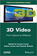
Figure 4.3. Characterization of geometry of the 3D multiscopic display using colocalized planar mixing

Our analysis of the characteristics of viewing geometry relies on a global reference frame defined in relation to the display device r = (CS, x, y, z ≡ x ∧ y), selected at the center CS of the ROI with the axis x, parallel to the ROI’s lines and directed toward the viewer(s) right side, and the axis y, parallel to the ROI columns and directed toward the bottom.

The 3D display system mixes n × m images within its ROI with the dimensions L (width) and H (height). Each of these images (denoted by is presumed to be “correctly” visible (without being mixed with other images), at least from the preferred selected position O_i. These positions are arranged as m lines parallel to the ROI lines situated at a distance of d_i2 from the system’s ROI. Preferential positions are placed on these lines to ensure that the viewer, whose binocular gap is b_i2, with the eyes parallel to the lines on the display, will have his/her right eye at O_i and his/her left eye at O_gi. The parameter b_i2 is often identical to the average human binocular gap of 65 mm but it is possible to select a different gap depending on the target audience, i.e. children. The right eye at O_i will see image number i while the left eye O_gi will see image number g_i, knowing that g_i = i – (q_i2,0) where q_i2 represents the gap between image numbers composing coherent stereoscopic couples that are visible with a binocular gap of b_i2 with a distance of d_i2. As such, by combining the preferential positions of both the left and right eyes, we have: O_i = O_gi + b_i2 x and o_i = o_gi + b_i2.

We also place the preferential position lines on the vertical axis by p_i2, which represents the drop, i.e. the vertical gap between line i₂ of preferential positions and the center CS of the ROI. When m = 1, the device does not create any vertical separation and any drop is acceptable a priori. However, not all drops create the same perception and it is therefore necessary to know the average effective drop of target viewers during the design stage. If we do not know this expected drop p_i2, we use the drop of an average size viewer.

Supposing that the pixels u_i and u_gi are stereoscopic homologues in the images i and g_i, their perception by the right and left eye at O_i and O_gi leads the viewer’s brain to perceive the 3D point v by stereopsis.

4.3. The geometry of 3D shooting

4.3.1. Choosing a convenient geometry

Providing 3D content to selected display systems requires sets of n × m images of a scene obtained using well-selected distinct points of view according to adapted projective geometries. A correctly positioned viewer will therefore receive two distinct images that form a stereoscopic couple that allows his brain to perceive the scene depth. Each eye receives an image that physically originates from the same area (which is normally rectangular), which corresponds to the display’s ROI. What differs is that each eye is evidently positioned differently and therefore views the device’s ROI according to different target axes. Depending on the desired application, three types of multiview shooting geometries are used primarily: convergent geometry, parallel geometry and decentered parallel geometry (see Figure 4.4).

Figure 4.4. The different shooting geometries represented in reversed pinhole model

Convergent shooting geometry (see Figure 4.4(a)) relates to cameras whose optical axes, equivalent to the target axes², converge at a single point without a shared base for shooting pyramids. Solutions for this type of system have been proposed [SON 07, YAM 97]. Since images have different trapezoid distortions, it is necessary to apply a systematic trapezoid correction to enable the perception of 3D. However, this is not necessarily desirable due to the fact that it slows the chain of production and deteriorates the quality of images.

Another standard geometry, known as parallel (see Figure 4.4(b)), involves optical axes, equivalent to the target axes, parallel with each other, passing by optical centers aligned on m “optical center” straight lines parallel to the sensors’ lines. It can be considered as a specific example of convergent geometry (with an infinite distance of convergence), as well as a specific decentered parallel geometry (with null decentering). If it does not require any prior correction in the images to enable 3D perception, this configuration is not entirely the best suited. Indeed, the perceived scene only appears to be protruding from the display since all the captured points are in front of the point of convergence at infinity, which is reproduced at the center of the display’s ROI.

Lastly, decentered parallel shooting geometry (see Figure 4.4(c)) shares features with parallel geometry (parallel optical axes, optical centers aligned on m straight lines parallel to the sensors’ lines) but separates the optical axes that converge at infinity and target axes that converge at a single point in the scene. As a result, the convergence distance of the target axes is no longer necessarily infinite. This is achieved by decentering the actually-used zone on each sensor (capture area) so that its center is aligned with the optical center and the chosen point of convergence. The visualization pyramids are therefore decentered and share a rectangular base, a projection of their capture area via their optical center on the plane parallel to the sensors passing by the point of convergence. Since their apices (optical centers) are distributed along a straight line parallel to the lines of this shared base (see Figure 4.5), these image shooting pyramids correspond qualitatively to those of the target display devices. With the shared base being displayed on the display’s ROI, it is possible to render a scene both protruding (points in front of the point of convergence, perceived in front of the ROI) and hollow (points behind the point of convergence, perceived behind the ROI). Dodgson et al. have used this scheme for their autostereoscopic camera system with temporal multiplexing [DOD 97].

Figure 4.5. Generic description of a decentered parallel geometry

As we have seen, display on a flat multiscopic system involves selecting, for the two images aimed at the same viewer, capture pyramids sharing a rectangular base in the scene with apices placed on a straight line parallel to the lines in this shared base. For contexts of collective viewing of a single scene (autostereoscopic systems), which share views between several potential observation positions within one or several “chains” of key positions, this shared base should be applied to all captures destined for this single chain and even all chains if we want coherence between viewing of these different chains. The target axes are therefore all necessarily convergent at the center of this shared base and the apices of the pyramids must pairwise form straight lines parallel to the shared base’s lines. Each “chain” of images must therefore be captured from positions located on a straight line parallel with the lines of the shared base. As such, so that the capture areas yielding to these pyramids and therefore the images that they capture remain rectangular, they must be parallel to this shared base. We must thus use a decentered parallel system (see Figure 4.4(c)), as Yamanoue and Woods have shown [WOO 93, YAM 06].

4.3.2. Setting the parametric model

Figure 4.6 provides a perspective representation of a decentered parallel shooting geometry. This figure shows the plane of the capture areas (ZC_i) and the optical centers (C_i) and specifies a set of parameters that completely characterize the shooting geometry. Figures 4.6(b) and (c) show the view from above and the front view of this geometry.

Figure 4.6. Characterization of the decentered parallel shooting geometry

Our analysis of shooting geometry relies on the global shooting reference frame R =(PC, X, Y, Z ≡ X ∧ Y) , which is centered at the desired point of convergence PC (which is also the center of the shared base BC in the scene) and is directed so that the first referential vectors are colinear to the axes of the shared base BC in the scene and are therefore colinear with the axes in the capture areas. In addition, the first axis is presumed to be parallel to the lines in the capture areas and the second axis is parallel to the columns in these areas. The size of the shared base BC has the dimensions Lb and Hb. This reference frame defines the position and direction of all the projection pyramids representing the capture areas by specifying the direction of observation Z and the m alignment lines of the optical centers.

In line with these principles, the n × m shooting pyramids are specified by:

– optical axes in the direction Z;

– the optical centers Ci aligned on one or several (m) straight lines parallel to the lines in the shared base and therefore the direction X;

– rectangular capture areas ZC_i.

The capture areas must be orthogonal to Z and therefore parallel to each other and the shared base BC as well as the straight lines holding the optical centers C_i (which are defined by their distances to PC, D_i2 in relation to Z, P_i2 in relation to Y and c_i in relation to X). These capture areas are placed at distances of f_i in relation to Z, β_i in relation to Y and α_i in relation to X from their respective optical centers C_i. Their dimensions are l_i and h_i. They are decentered in relation to their respective optical axes in the points I_i such that the straight lines (I_iC_i) define the target axes intersecting at the fixed point of convergence PC. The centers C_i and Cg_i must be on the same “center line” and spaced from B_i in relation to X (C_i = C_gi + B_iX and c_i = c_gi + B_i).

This kind of shooting configuration ensures a depth perception on a multiscopic system with colocalized planar mixing with the possibility of a protruding as well as hollow image effect. However, this does not ensure that the perceived scene will not be distorted in relation to the original scene. The absence of distortion implies that the viewing pyramids are perfect homologues of the shooting pyramids, i.e. they have exactly the same opening and deviation angles in both horizontal and vertical directions. Any flaw in this shooting and viewing pyramids’ homology involves a potentially complex distortion of the 3D image perceived in relation to the captured scene. In some cases, however, this is desirable when creating special effects among other things. This implies that the shooting and viewing configurations must be specified as a set, which must ensure the desired distortion (or non-distortion) effect.

We will now model these distortion effects that are potentially implied by the combination of shooting and viewing geometries.

4.4. Geometric impact of the 3D workflow

4.4.1. Rendered-to-shot space mapping

In this section, we will use perfect lenses and sensors without distortion.

According to our analyses of viewing and shooting geometries, it is possible to connect the coordinates (X, Y, Z), in the reference frame R, from the point V in the scene captured by the previously identified cameras with the coordinates (x_i,y_i,z_i) in the reference frame r of its homologue v_i perceived by an observer of the display device, placed in a preferential position (the right eye at O_i). Supposing that the point V in the scene is visible in image number i, its projection U_i verifies:

[4.1]

Knowing that I_i, the center of ZC_i, is the projection on the image i of PC, the center of R, we can calculate I_i – C_i. By subtracting this result from equation [4.1], we obtain the positions of the projections of the point V in the different images:

[4.2]

Since the images are captured downward the optical centers, the images’ implicit axes are the opposite of those in the global shooting reference frame R. In addition, the images are resized for display according to the display device’s ROI. This places the projections U_i of V at their positions u_i on the ROI:

[4.3]

Thalès’ theorem used in Figure 4.6 yields f_iL_b = D_i2l_i and f_iH_b = D_i2 h_i. Therefore, we express u_i in the reference frame r by:

[4.4]

Let us remark that the image g_i comes from the sensor associated with the optical center C_gi, which is on the same “centers’ line” that the optical centers as C_i (same secondary index i₂) and is spaced from B_i in relation to X (C_i = C_gi + B_iX and c_i = c_gi + B_i). Then, supposing that V is visible in the two images g_i and i, we can see that u_gi and u_i are situated on the same line of the ROI. This responds to the epipolar constraint and therefore enables the stereopsis reconstruction of from O_gi and O_i. In Figure 4.3, Thalès’ theorem gives us:

[4.5]

By inverse projection, we find v_i:

[4.6]

Therefore, the relation between the 3D coordinates of points at the scene and those of their images perceived by the viewer at position number i can be characterized by:

[4.7]

Since a_i affinely depends on Z, we progress onto homogeneous 4D coordinates:

[4.8]

Equation [4.8], corresponds to the transformation matrix given by Jones et al. [JON 01], with a characterization of distortion parameters depending on the shooting and viewing parameters in the analytical distortion model for a viewer at position i.

4.4.2. 3D space distortion model

This model (see equation [4.8]) clearly highlights all the distortions that could be obtained during a multiscopic viewing experience using planar colocalized mixing systems, regardless of the number of views or the nature of the images (whether real or virtual). It also underlines, in addition to a_i (leftover calculation with no other significance), new parameters that quantify their distortions. Homogeneous matrices therefore define the transformations between the initial space in the scene and the viewing space for each favored observation position numbered as i. These parameters can be analytically expressed using geometric parameters from shooting and viewing systems. Their relations with the geometric parameters are presented in Table 4.1 and their impacts on distortion are described below:

– k_i2: the global magnification factor, which does not really distort the scene.

– ε_i: the control parameter of the potential nonlinear distortion, which transforms a cube in a truncated pyramid of the axis Z. Depending on the rate of global reduction , which can vary according to Z, if ε_i ≠ 1, this creates a distortion in the displayed volume as a “truncated pyramid” of the axis Z.

–μ_i : the rate of width magnification in relation to the depth. When μ_i ≠ 1, a horizontal/depth anamorphosis producing unequal dilations in X in relation to Z is applied.

– ρ: the rate of height magnification in relation to width. When ρ ≠1,a vertical/horizontal anamorphosis producing unequal dilations in Y in relation to X is applied.

– γ_i: the horizontal/depth skew of the perceived scene. When γ_i ≠ 0,a horizontal drift according to the depth is applied.

– δ_i: the rate of vertical/depth skew of the scene perceived by a viewer of a drop conforms to expectations. When δ_i ≠ 0 and/or when the viewer’s real drop differs from the optimal drop, a vertical drift according to depth is applied.

Table 4.1. Expression of parameters quantifying the distortions in relation to shooting and viewing geometric parameters

This defines all the depth distortion possibilities using the previously established shooting and viewing geometries. In addition, this model quantifies these distortions for any pair of settings (shooting and viewing) by a simple calculation based on their geometric parameters.

4.5. Specification methodology for multiscopic shooting

In this section, we propose a methodology that specifies the shooting configuration required to obtain the desired 3D distortion on a given display system [PRE 10]: a perfect 3D effect or selected distortions. Indeed, knowing how the distortion, shooting and display parameters are related, it is possible to adapt the shooting to the choice for distortions and viewing. We describe two shooting schemes using the distortion model: a generic scheme that gives precise control of each distortion parameter, and a second more specific, but very significant, scheme since it is involved in creating accurate depth perception (i.e. without any distortion).

4.5.1. Controlling depth distortion

It is possible to calculate the ideal shooting configuration for a desired distortion and fixed display. To do so, we have a range of distortion parameters that can be defined according to the desired result. By adjusting the magnification factor k_i2 and by fixing the distortion parameters ε_i (and therefore a_i = ε_i + k_i2 (ε_i – 1) /d_i2), μ_i, ρ, γ_i and δ_i, we obtain the desired 3D distortion. The last condition on δ_i is more difficult when m = 1 because this depends on the height of the viewer, which inevitably affects the real viewing drop (height of the eyes in relation to the center of the device) in relation to the display system. The selected vertical skew δ_i can therefore only be obtained in this case for a viewer whose real drop corresponds to that defined in the viewing rules for this viewing position.

Using the desired viewing and distortion parameters, it is possible to calculate the shooting parameters, which ensure that the desired distortion is obtained effectively by displaying on the chosen 3D device. The equations used, obtained by inverting those which define the distortion parameters, are given in Table 4.2.

This control scheme for depth distortion obtains shooting parameters that produce the desired content for any colocalized planar mixing multiscopic display system and any combination of depth distortions according to the model in equation [4.8]. This can prove highly useful within the cinema and the special effects’ industry where we may want to accentuate 3D effect in certain parts of the scene to draw the viewer’s attention.

Table 4.2. Shooting parameters in the case of controlling depth distortion and in the case of accurate depth. The darkroom depth f_i can be imposed or chosen (globally – by center line, – or individually, )

4.5.2. Accurate depth effect

A specific example of depth distortion is perfect or accurate depth (a perception of the scene without any distortion in comparison to the real scene). To do so, it is necessary that the shooting of images, the display device’s configuration (its ROI) and the conditions of use (favored positions) are jointly defined according to the desired distortion parameters. To create an accurate depth display (with a global magnification factor k_i2), we need to configure the shooting in order to prevent potential distortions. This is achieved by ensuring that the distortion parameters verify ε_i = 1, μ_i = 1, ρ =1, γ_i = 0 and δ_i = 0. This last condition, δ_i = 0, is more difficult if m = 1 because it depends on the height of the viewer, which inevitably affects the effective drop in relation to the device. It can therefore only be guaranteed for viewers with a real drop equal to that defined in the display parameters for this viewing position. The shooting configuration parameters can therefore be calculated by replacing the distortion parameters fixed previously. The equations used are provided in Table 4.2.

This specific case is highly interesting due to its realism and has a number of potential applications. This is particularly the case, for example, with medical visualization software where accurate display is essential for a correct diagnosis or computer aided design (CAD) software that eliminates interpretation errors when designing a mechanical part. It could also be used to convince investors or planning committees by giving a 3D impression of the real size of a building.

4.6. OpenGL implementation

The shooting specification method examined previously can be used to develop OpenGL applications that can render 3D media. This method places virtual cameras around a standard monocular camera depending on the chosen display device and the desired depth effect. The advantage of this virtual scheme is that virtual cameras are perfect and there is therefore no problem with potential distortions due to sensors or lenses. The camera arrangement in OpenGL is explained below.

The geometry of a single camera is normally defined by its position, direction and vision pyramid. However, in stereoscopic environments, it is necessary to have two virtual cameras, one for each eye, whereas multiview autostereoscopic displays require up to N virtual cameras. Each virtual camera is laterally shifted and has its own decentered pyramid of vision such that the center of its image is located on the line linking its optical center and the center of convergence lying on the optical axis of the reference monocular camera. The optical axes are parallel to each other. The distance of the “depth-clipping” planes, i.e. the planes perpendicular to the optical axes between which the objects are viewed, remains unchanged. The convergence distance (depth of the convergence point) must be manually defined. This determines whether the objects appear “in front of” or “behind” the display, thereby creating (or not) a protruding effect.

Algorithm 4.1, identifies the six parameters l, r, b, t, n, f required by the OpenGL function glFrustum: l and r are the coordinates (left and right) of the vertical “clipping” planes, b and t are the coordinates (top and bottom) of the horizontal “clipping” planes and n and f are the distances of the depth “clipping” planes.

We then apply the OpenGL command chain to correctly place the camera and therefore obtain the desired view. As such, we can create the N views desired by varying c from 0 to N – 1. The use of these views depends on the autostereoscopic display device chosen and is examined in Chapter 14.

Algorithm 4.1. Obtaining N views

4.7. Conclusion

In this chapter, we have examined a methodology that can be used to describe and qualify the geometric relations linking a 3D shooting device with a display device mixing 3D colocalized planar images. These relations, defined by a restricted set of parameters, provide global control of distortions and can be used to specify the shooting geometry, which will guarantee, for both a real and a virtual scene, that the images will be accurately displayed on a given 3DTV device. Principally aimed at autostereoscopy, this chapter can be applied to a number of areas in 3D visualization in line with, for example, biomedical imaging, audiovisual production and multimedia production.

4.8. Bibliography

[DOD 97] DODGSON N.A., MOORE J.R., LANG S.R., “Time-multiplexed autostereoscopic camera system”, Proceedings of Stereoscopic Displays and Virtual Reality Systems IV, SPIE, vol. 3012, 1997.

[DOD 02] DODGSON N.A., “Analysis of the viewing zone of multi-view autostereoscopic displays”, Proceedings of Stereoscopic Displays and Applications XIII, SPIE, vol. 4660, pp. 254–265, 2002.

[DUB 01] DUBOIS E., “A projection method to generate anaglyph stereo images”, Proceedings of the IEEE International Conference on Acoustics, Speech, and Signal Processing, IEEE Computer Society Press, pp. 1661–1664, 2001.

[HIL 53] HILL A.J., “A mathematical and experimental foundation for stereoscopic photography”, Journal of SMPTE, vol. 61, pp. 461–486, 1953.

[JON 01] JONES G., LEE D., HOLLIMAN N., et al., “Controlling perceived depth in stereoscopic images”, Proceedings of Stereoscopic Displays and Virtual Reality Systems VIII, vol. 4297, pp. 42–53, June 2001.

[PEI 09] PEINSIPP-BYMA E., REHFELD N., ECK R., “Evaluation of stereoscopic 3D displays for image analysis tasks”, in WOODS A.J., HOLLIMAN N.S., MERRITT J.O. (eds), Stereoscopic Displays and Applications XX, SPIE, pp. 72370L–72370L–12, 2009.

[PER 00] PERLIN K., PAXIA S., KOLLIN J.S., “An autostereoscopic display”, ACM SIGGRAPH 2000 Conference Proceedings, vol. 33, pp. 319–326, 2000.

[PRE 10] PRÉVOTEAU J., CHALENÇON-PIOTIN S., DEBONS D., et al., “Multiview shooting geometry for multiscopic rendering with controlled distortion”, International Journal of Digital Multimedia Broadcasting (IJDMB), special issue Advances in 3DTV: Theory and Practice, vol. 2010, pp. 1–11, March 2010.

[SAN 03] SANDERS W.R., MCALLISTER D.F., “Producing anaglyphs from synthetic images”, in WOODS A.J., BOLAS M.T., MERRITT J.O., BENTON S.A. (eds), Stereoscopic Displays and Virtual Reality Systems X, SPIE, pp. 348–358, 2003.

[SON 07] SON J.-Y., GRUTS Y.N., KWACK K.-D., et al., “Stereoscopic image distortion in radial camera and projector configurations”, Journal of the Optical Society of America A, vol. 24, pp. 643–650, 2007.

[WOO 93] WOODS A., DOCHERTY T., KOCH R., “Image distortions in stereoscopic video systems”, Proceedings of SPIE: Stereoscopic Dispalys and Applications IV, vol. 1915, pp. 36–48, 1993.

[YAM 97] YAMANOUE H., “The relation between size distortion and shooting conditions for stereoscopic images”, SMPTE Journal, vol. 106, pp. 225–232, 1997.

[YAM 06] YAMANOUE H., “The differences between toed-in camera configurations and parallel camera configurations in shooting stereoscopic images”, IEEE International Conference on Multimedia and Expo, vol. 0, IEEE Computer Society, pp. 1701–1704, 2006.

1 An optical beam is a series of light rays emanating from a single wide source, which may be a screen, projector or another source. However, only its restriction to a single point source on the display is shown in Figure 4.1(a).

2 The optical axis is the line orthogonal to the sensor passing by the optical center while the target axis is the line passing through the optical center and the center of the sensor’s ROI.

Chapter written by Jessica PRÉVOTEAU, Laurent LUCAS and Yannick REMION.