Chapter 6

Feature Points Detection and Image Matching

6.1. Introduction

Image matching is a part of many computer vision or image processing applications, such as object recognition, registration, panoramic images and image mosaics, three-dimensional (3D) reconstruction and modeling, stereovision or even indexing and searching for images via content. The problem is finding the geometric transformation (rigid, affine, homographic or projective) that best matches two images using visual information shared by the two images. The main hypothesis is that the visible part of the 3D object from a given angle is almost identical to that obtained from another angle.

The different matching techniques vary according to the number and the nature of visual information used. When all the pixels in the image are used, matching is dense. Within the context of medical image registration, this may relate to landmarks, precisely defined anatomical points [ROM 02], or “semi-landmarks” [BER 04]: the amount of visual information used is minimal but matching is preceded by a landmark recognition stage. This chapter will examine a general scenario where the amount of visual information is limited and where no prior knowledge is available.

This visual information corresponds to regions detected using specific photometric or geometric properties such as edges, corners or “blobs”. They are represented by local descriptors often based on local photometry. Matching visual elements shared by two images is carried out by comparing their descriptors using adapted metrics or by classification. The transformation between the two images can therefore be calculated using these elements. The current process consists of three main stages:

6.2. Feature points

There is a wide body of literature [AWR 12, GAU 11, MIK 05a, MOK 06, ROM 12, TUY 08] on feature point extraction. Local information searches have been largely motivated by the unreliability of global object representations in terms of occlusion, articulated objects, intensity or viewpoint variations, robustness to noise acquisition (sampling, shaking, blur, etc.) and detection accuracy. The detection and representation of obtained points/regions must be invariant, particularly in terms of:

The local nature of detectors lends a certain robustness to occlusions and local deformations. It is the spatial organization of these points that characterizes an object. They must therefore be fairly numerous and discriminative in order to uniquely describe an object. Lighting and viewpoint invariant properties are ensured by detectors and descriptors. One feature point can be assimilated with a pattern in the image that differs from its neighbor due to its photometric properties (intensity, color, texture, etc.), its specific local form or even its segmentation stability. These include points, lines or regions.

6.2.1. Point detection

6.2.1.1. Differential operators: autocorrelation, Harris and Hessian

Historically, objectives of repeatability/robustness, precise location, and informative and understandable content have resulted in the study of variations in intensity function S(x, y). In this context, the first corner detector was developed by Moravec [MOR 81].

It calculates the windowed neighborhood autocorrelation for each point as follows:

where w(x, y) is a weighting function. It detects the local maxima in all directions of the autocorrelation function. However, this simple detector is very sensitive to noise in the image, particularly near its edges, thereby favoring directions in the image frame.

To overcome these disadvantages, Harris [HAR 88] used a second-order development of S(x, y) and a Gaussian weighting function G to decrease its sensitivity to noise and suppress anisotropy. Therefore, the function E becomes:

with:

The matrix A is a positive-definite matrix whose eigenvectors v_max and v_min associated with the eigenvalues λ_max and λ_min provide information about the directions of local intensity changes: the vector v_max (respectively, v_min) is associated with rapid changes in intensity (respectively, slow) and is perpendicular (respectively, parallel) to the edge. When these two eigenvalues are small, the pixel is in a homogeneous zone; when only one eigenvalue is high, it is an edge; and when the two eigenvalues are large, it is a corner. To avoid the costly calculation of eigenvalues, Harris has proposed using the following measure:

The function E(x, y) is high and positive for a corner and negative or nul otherwise. α is approximately 0.04 and is defined empirically. The feature points retained by the Harris detector correspond to the local maxima of the function E(x, y). This corner detector is invariant to translations, rotations and affine intensity variations. However, it is affected by scale and affine transformations. An example using this detectoris shown in Figure 6.1(a).

An alternative solution based on derivatives has been proposed by Beaudet [BEA 87]. It involves determining the maximal values of the Hessian matrix determinant.

Considering the image function S as a curved surface in ³, the curvatures of the surface [REN 00] are studied. This operator is invariant to rotation but is sensitive to noise as it is based on second-order differential operators. An improvement can be made by a Gaussian smoothing and a selection of points where the trace of the Hessian is a local extremum. This operator shows the same invariances as the Harrris operator and detects “blobs”. An example of detection using the Hessian detector is illustrated in Figure 6.1(b).

6.2.1.2. Scale invariance using multi-scale analysis

Detectors such as Harris and Hessian use a measure based on a smoothing dependent parameter: scale. They detect the points or regions at a single scale. Since this scale is a priori unknown, multi-scale approaches automatically determine the correct scale. Lindeberg [LIN 08] has shown that the Gaussian kernel is the only linear smoothing that provides a correct multi-scale analysis. Current detectors construct a Gaussian pyramid, calculate a spatial measure of interest normalized for each pixel and level in the pyramid, and detect the extrema localized in x, y, σ in this 3D “spatial-scale space”.

The Scale-Invariant Feature Transform (SIFT) detector [LOW 04] uses the Gaussian Laplacian as a saliency measure and looks for the extrema of this measure in the 3D space x, y, σ. Feature points with weak contrasts are eliminated along with feature points near low curvature edges (see Figure 6.2(a)). To reduce the algorithmic cost of this approach, the Gaussian Laplacian is approximated using Gaussian differences. This approximation only slightly affects the detector’s performance and remains a reference tool. The Speeded-Up Robust Features (SURF) detector [BAY 08] uses a Hessian approximation as a spatial measure and is much faster. It replaces Gaussian smoothing with “box filters”. These filters are composed of three or four blocks whose coefficients are identical inside a block. The integral image is then used to calculate convolution making this detector highly efficient (see Figure 6.2(b)).

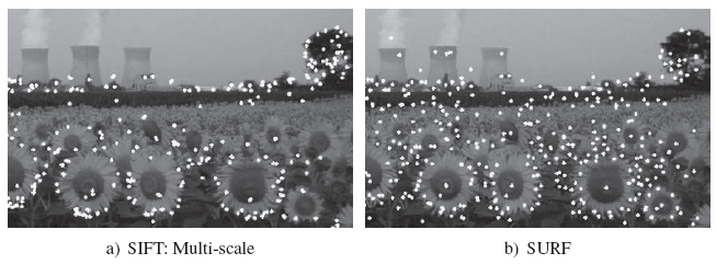
The main disadvantage of these detectors is that they respond fairly strongly to edges, particularly for the Laplacian. They are, however, a reference tool in feature point detection. To ensure scale invariance, they are included in multi-scale analysis. This analysis can be used to define the scale where saliency is maximal and therefore has the most stable value. They have good “blob” and corner detectability, with the exception of junctions between several areas.

6.2.1.3. A corner intensity model

The Smallest Univalue Segment Assimilating Nucleus (SUSAN) detector [SMI 97] uses the following property. We separate the circular neighborhood pixels from a sample pixel into two parts: those whose intensity is similar and those whose intensity is far from that in the sample pixel. Intuitively, a homogeneous region partitions the neighborhood into an empty zone and a zone of identical size to that of the neighborhood used, an edge partitions it into two zones of equal sizes and a corner partitions it into two zones of different sizes (25% and 75%). SUSAN calculates the number of pixels (known as USAN) similar to the pixel intensity by a given threshold. For a corner, this number must be less than half the window size. False positive detections are eliminated by checking the distance between the USAN center of gravity and the sample pixel that must be sufficient to validate the corner. SUSAN’s primary disadvantage is its sensitivity to blurry edges whose corners are poorly detected. This detector is also less robust to noise near edges, depending on the size of the mask used. This is evident in Figure 6.3 where, despite adjusting the parameters, the number of corners detected is fewer in the right image that is blurred. The SUSAN detector is almost invariant to lighting conditions and is, in particular, fast.

Designed for real-time applications, the Feature from Accelerated Segment Test (FAST) detector [ROS 05] uses the same principle with a lower computational cost. A point is considered to be a corner when a large number n of connected points situated on a circle (and not a disk, as with SUSAN) are clearer or darker than the central point. These connected sets are denoted as E_clear and E_dark. The initial parameters are fixed at a radius of 3 pixels for a discrete circle of 16 pixels and n = 12. To optimize the algorithmic cost, tests are prioritized following the order of the neighboring positions: north, south, east and west. At least three of them must be clear in order for the studied point to be a corner. The other pixels are only examined if this test is verified. To eliminate multiple responses to a single corner, the non-maximal values of the following score V are removed:

An improved version [ROS 10] replaces the static tests with a decision tree that is automatically constructed by learning from a set of training images. Learning is based on an entropy criterion. This fast and high performing detector has become a standard for real-time applications. It is, however, sensitive to blurring, as is the SUSAN detector.

Scale invariance is achieved by the Binary Robust Invariant Scalable Keypoints (BRISK) detector, which combines the scale space and the FAST approaches [LEU 11]. In this algorithm, only a few scale levels are considered, thereby limiting computational cost. However, a quadratic interpolation between scales is applied. BRISK has detection performance comparable to SURF and SIFT, with the exception of blurred images, with six times lower computation cost than SURF and 10 times lower computation cost than SIFT.

6.2.2. Edge-based feature points

Another class of detectors operates according to image edges. Edges are fairly stable objects in relation to changes in perspective and lighting conditions. These detectors also use local geometry, straight lines and parallelograms for the “Edge-Based Regions” (EBR) operator or curvature for the “Curvature Scale Space” (CSS) operator.

6.2.2.1. Shape detectors

The EBR operator [TUY 04] initially locates corners using the Harris detector and then detects the edges using a Deriche operator. If we consider a corner p, then two points p₁(l₁) and p₂(1₂) move along the edges sharing this corner. The curvilinear distance p_1,2 of each point p_1,2 at the corner p is defined as the surface between the edge and straight line joining the corner and the point p_1,2. This distance is invariant to affine transformations. These two points and the corner define a family of parallelograms. The retained parallelogram is the one that shows an extremum value of a photometric function based on the first-order points from the intensity function. This operator locates parallelepiped forms that are invariant to affine geometric and photometric transformations (see Figure 6.4(a)).

For these detectors, the primitives (parallelepiped) mean that they are designed primarily for structured scenes with artificial or well-contrasted elements.

6.2.2.2. Curvature and scale space

The CSS [MOK 98] searches for the extrema of the curvature function along the edges using a multi-scale approach. It detects edges using the Canny operator first, fuses the close edges and then calculates the curvature K(t, σ) smoothed by a Gaussian defining the curvature space.

The corners are the extrema in this space. Those with a too low value or which are too close to other corners are not retained (see Figure 6.4(b)). A variant of this detector [MOK 01] differentiates the analysis of short curvatures and long curvatures by automatically determining the decision threshold. This operator is invariant to affine geometric and photometric transformations.

The primary disadvantage of these edge-based detectors is the definition of parameters used by the edge detector. As shown in Figure 6.4 some corners are not detected when edges are slightly contrasted.

6.2.3. Stable regions: IBR and MSER

The “Intensity Based Regions” (IBR) detector [TUY 04] detects the local extrema of the image intensity S. It then explores the area around each of the extrema by studying an intensity function along the rays traced from the local extremum. For each ray, the following function is evaluated:

where t is the curvilinear abscissa along the ray and d is a small number that prevents divisions by 0. The extrema of this function for each ray are chained and form a closed area. The denominator ensures good localization of extrema. This region is then approximated by an ellipse. This operator detects “blobs” and is robust, particularly for printed documents. It is invariant to affine geometric and photometric transformations.

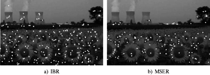
The “Maximally Stable Extremal Regions” (MSER) detector [MAT 02] relies on the idea that as intensity varies strongly along the edges of objects, their subgraph varies slightly according to this intensity. The regions considered by this detector are therefore the connected components in the thresholded image whose surface varies slightly according to this threshold. They are detected by a watershed algorithm in which the watershed surfaces are analyzed. These regions are invariant to monotone intensity transformations (and not only photometric affine transformations), to homographic geometric transformations and to continuous geometric rather than linear transformations. This detector is robust, efficient and fast. Its only disadvantage is its sensitivity to blurring because in this case the intensity at the edges is poorly defined and the extremum threshold is very poorly localized.

Region-based detectors do not detect corners or angles in the image. They consider the center of the detected regions as the point of interest, as shown in Figure 6.5 (particularly in the sunflowers’ heads).

6.3. Feature point descriptors

A description of the local content of these points is necessary to differentiate them within the context of image matching. In the literature, there are a number of description methods that have been proposed and have resulted in the computation of descriptor vectors for each point. A point’s descriptor indicates the distribution of information in a region centered at the keypoint. These descriptors are designed to be invariant to small deformations, localization errors and rigid or affine transformations as well as illumination changes. The choice of a descriptor size is important and has a direct impact on the speed and cost of matching. Low dimensional descriptors are often less discriminatory but faster and are a source of complexity in the matching stage. They are therefore best suited to real-time contexts.

6.3.1. Scale-invariant feature transform

The SIFT descriptor was introduced by Lowe [LOW 99] and has become the most commonly used descriptor due to its robustness and computation time. It describes the distribution of gradients within a region around the feature point. This approach ensures scale and rotation invariance. The feature point detection scale is used to define the size of the window in which the descriptor is calculated. Each gradient magnitude m(x,y) is weighted by a Gaussian distance centered on the feature point with a standard deviation 1, 5 times the scale σ of the point:

where d_x and d_y are the distances in x and y directions at the feature point descriptor window.

The descriptor window is rotated relative to the dominant orientation to achieve a rotation invariance of the SIFT descriptor (see Figure 6.6). This orientation is obtained by analyzing the orientation histogram. The descriptor window is subdivided into 4 × 4 subregions. An orientation histogram (eight orientations at 45 degrees intervals) is then calculated for each subregion. The different histograms are stored in a 4 × 4 × 8 = 128 dimensional vector. The descriptor vector is then normalized to achieve invariance to changes in illumination. To reduce the influence of large gradient magnitudes on the descriptor, the values in the descriptor vector are thresholded and those above 0.2 are restricted to this value. The descriptor vector is then normalized to unit length.

6.3.2. Gradient Location and Orientation Histogram

Similar to the SIFT descriptor, the Gradient Location and Orientation Histogram (GLOH) descriptor [MIK 05b] indicates the distribution of intensity gradients in the local region around the feature point. This is represented by a polar grid of 17 subregions (see Figure 6.7) (a central circular region and 8 × 8 subregions with intervals of on two circular regions centered on the keypoint).

For each of these subregions, a gradient histogram of 16 bins is calculated to produce a descriptor vector with 17 × 16 = 272 dimensions.

6.3.3. The DAISY descriptor

The DAISY descriptor [TOL 10] is similar to the SIFT and GLOH descriptors. Their main difference lies in the shape of the region in which the descriptor vector is calculated. This region is composed of several overlapping circles centered on the feature point (see Figure 6.8): the radii of the circular grids are proportional to the distance of the Gaussian kernels from the feature point and the Gaussian smoothing is proportional to the circles’ radii. For each circular region, an orientation histogram is calculated and normalized. The descriptor vector is the result of the concatenation of all the orientation histograms and is of high dimensionality (544). Due to the shape of its computation area, the DAISY descriptor is invariant to rotation. Therefore, it has the advantage of being able to be redefined in different orientations without the need to compute convolutions. This descriptor outperforms previously presented descriptors in dense matching applications and has a low computation time.

6.3.4. Speeded-Up Robust Features (SURF)

As was the case for the SIFT descriptor, the SURF descriptor [BAY 08] describes the distribution of intensities in the neighborhood of the feature point. It has a low computation time due to the use of the integral image [VIO 01], which is used to estimate derivatives using first-order Haar wavelet filters.

The SURF descriptor is scale and rotation invariant. The detection scale defines the size of the descriptor window as well as the size of the filters. Within the descriptor window, the wavelet responses in the x and y directions are calculated and weighted by a Gaussian of 3.3 times the detection scale (see Figure 6.9). For each pixel in the descriptor window, an orientation vector is calculated and the maximal orientation is identified as the dominant orientation, sum of all responses within a sliding orientation window covering an angle of , around the feature point. The descriptor window is orientated relative to the dominant orientation and subdivided into 4 × 4 subregions. For each of these subregions, the four following values are calculated: , where d_x and d_y are the responses to the first-order Haar filters in the x and y directions, respectively (see Figure 6.9).

The descriptor vector is obtained by concatenation of these four values for each of the subregions. The final vector with a size of 64 is normalized to ensure invariance to contrast.

6.3.5. Multi-scale Oriented Patches (MOPS)

As with the SIFT descriptor, the MOPS descriptor [BRO 05] uses gradients to extract a dominant orientation in a region centered at the feature point. A patch of 8 × 8 pixels using a spacing of 5 pixels is sampled. The 64 dimensional vector is then normalized. A Haar wavelet transform is applied to this vector to obtain a descriptor vector containing the wavelet coefficients. This descriptor is invariant to small changes in intensity.

6.3.6. Shape context

The “shape context” descriptor [BEL 00] is based on the idea that a shape is associated with an object. A shape is described by a discrete subset of its edge points. The “shape context” descriptor is a histogram of edges’ coordinates. It is calculated in the log-polar grid centered on an edge point, sampled as 5 (rings) × 12 (orientations) regions, similar to that of the GLOH descriptor. The shape context h_i in a selected edge point corresponds to the histogram of edge points that belong to each of these regions.

To provide a better description, the orientation is studied. In each region or “bin” k, the vectors t_j tangent to each of the points q_j in the edge Q belonging to the grid are calculated. The orientation is given by the sum of tangent vectors on each bin as follow:

t_j, where

This descriptor is known as “Generalized Shape Context” and contains the dominant histogram orientations of each region k of the grid.

6.4. Image matching

Matching between image feature descriptors is the classic approach used to compare or match images.

6.4.1. Descriptor matching

The matching process involves comparing the descriptors taken from an unknown image with the descriptors taken from a target image. This comparison relies on calculating a dissimilarity measure (for example, Euclidean or Mahalanobis distances) and a selection criterion. Maintaining correspondence between a new descriptor and one or several potential descriptors requires the implementation of a threshold on similarity distances. In practice, three approaches are used to determine the matching between two descriptors [MIK 05b]. All three approaches rely on an empirical threshold definition. The simplest approach uses a direct threshold on similarity distances. This threshold depends directly on the deformation in a scene, which means that this approach is not particularly robust. The following approaches use the spatial nearest neighbor concept to establish valid correspondences. In the second approach, a match is validated if the nearest neighbor has a similarity distance lower than the threshold. The last approach, introduced by Lowe [LOW 04], involves calculating a ratio between the similarity distances to the two nearest neighbors. This last approach penalizes descriptors that have several similar correspondents. For data sets of significant size, Lowe [LOW 04] proposes accelerating the search using “k-d tree” [FRI 77] or even “Best-Bin-First” [BEI 97] algorithms.

The weakness of these three matching approaches is the use of an empirically determined threshold. Each descriptor can be associated with exactly one known candidate descriptor. An alternative approach proposed by [RAB 08] avoids setting the detection threshold and the usual restriction to the nearest neighbor, allowing multiple matches between images. This means a match is rejected according to a dissimilarity criterion using the “Earth Mover Distance” [RUB 00], since this is less sensitive to the descriptor quantification problem. This matching criterion, called a contrario, involves detecting groups of descriptors whose existence is barely probable according to the hypothesis that these descriptors are independent of each other.

6.4.2. Correspondence group detection

Matching descriptors between two images, based on calculating their similarity, produces strong matches. However, a number of false correspondences are also retained. To remove them, a second stage is necessary. It involves estimating a geometric transformation by detecting groups of consistent correspondences. Therefore, the objective is to eliminate false matches while keeping a maximum of good correspondences. This task is, in particular, difficult when images are subject to strong deformations, occlusions or ambiguities (repetitive structures and absences of texture). Several groups of global methods provide a solution to this problem.

The complexity of matching is closely related to the geometric transformation that is considered during the matching stage. It is therefore necessary to study groups with a minimum of two correspondences to estimate similarity, three correspondences for affine transformation, four correspondences for homography and seven correspondences in the case of epipolar geometry.

6.4.2.1. Generalized Hough transform

The Hough transform [BAL 81, HOU 59] is an approach used to recognize small objects or strongly occluded objects within a scene. In these circumstances, Lowe [LOW 04] recommends using three descriptors to optimize the recognition process. The use of the generalized Hough transform identifies consistent groups of descriptors using the vote principle over samples of n correspondences. These votes are made within the scale space assigned to the parameters of the geometric transformation using quantified accumulators.

Given the high algorithmic complexity of this approach, it cannot be used for geometric transformations requiring more than three descriptor matches to be estimated, particularly if there is a particularly large amount of prior data. Estimating complex geometric transformations such as epipolar or even projective geometry can therefore be excluded from these approaches.

6.4.2.2. Graph matching

Graph matching is another tool that can be used to determine correspondences between descriptors using a global consistency criterion. The main idea here is to construct a graph whose descriptors correspond to the nodes and relations connecting them to the edges. High-level constraints, involving more than two descriptors, can be represented by hyperedges. Graph matching involves determining correspondences between the nodes of two graphs using matching constraints or by optimizing a global score.

Leordeanu and Hebert [LEO 05] have used the distance between two points as a constraint to ensure invariance to rotations. Berg et al. [BER 05] have used a criterion combining the notion of distance and angle, thereby ensuring scale and rotation invariance. Zheng and Doermann [ZHE 06] have proposed using the concept of neighborhood to define the matching constraint.

The more the order of graphs increases, the more precise the matching process and the more resistant it is to noise. In contrast to the previous approaches based on matching couples of points, point triplets are compared for third-order hypergraphs. [DUC 11, LEO 07, ZAS 08] have ensured invariance to various projections that include transformations in the similarity group, affine transformations or even projective transformations.

These approaches identify objects that have been subject to rigid deformation but can also be easily adapted to recognizing deformable objects. These methods, however, also prove fairly costly in terms of algorithmic complexity that increases with the order of the graph. They give good results provided the “inliers” represent at least 50% and the number of considered descriptors is relatively low (fewer than 100 in [DUC 11]).

6.4.2.3. RANSAC and its variants

The most commonly used method within the context of object recognition is the random sample consensus (RANSAC) algorithm [FIS 81] and its variants. This method effectively separates inliers from outliers. This approach consists of randomly sampling subsets of matches in order to predict the geometric transformation. The correspondences that are coherent with this model are therefore recorded. The set of correspondences yielding the maximal consensus is retained and represents the inliers while the others are considered to be outliers.

The strategy adopted in the RANSAC algorithm is fast and robust but requires regulating sensitive parameters. It is inconclusive when the rate ρ of inliers is low. This is due to the fact that the number of iterations required to randomly sample subsets is in the order of 1/ρⁿ, where n is the number of matches required to define the model. The strategies proposed in the MLESAC variants [TOR 00] or even PROgressive SAmple Consensus (PROSAC) [CHU 05] considerably reduce the number of models estimated while simplifying parameter regulation. However, they are not more effective than the original algorithm when ρ < 50%. The Optimized RANSAC (ORSA) algorithm [MOI 04] provides an effective solution to this problem when ρ is close to 10%. This last variant relies on the “a contrario” detection principle and overcomes the parameter setting in the case of epipolar geometry.

The previous RANSAC-derived methods all have a disadvantage when estimating the fundamental matrix. The outliers, whose corresponding features are near their epipolar line but far from their correct location, cannot be eliminated.

Moreover, the major disadvantage of these methods is the fact that detection is limited to a single object. To detect several objects, two strategies have been adopted in the literature: a simultaneous search of all object [TOR 00] or a sequential search that successively detects each object separately [STE 95]. In this context, MAC-RANSAC algorithm [RAB 08] proposes an automatic variant of the algorithm that sequentially detects multiple objects based on the “a contrario” detection principle.

6.5. Conclusion

Image matching is the key aspect in a number of applications such as image mosaics, panoramic images, object indexing or recognition, stereoscopy and 3D multiview reconstruction. In this context, the matching process is based on a non-dense approach that first requires the detection of feature points in the image, and then describes them using invariant descriptors. These descriptors are matched between images to estimate the transformation.

To detect corresponding points in images with different geometric and photometric characteristics, the detection stage uses a multi-scale approach of invariant spatial measurements. These measurements detect corners, blobs or even areas of random forms that are assimilated at their center. They are generally invariant to similarity group transformations and sometimes even to affine transformations. All detectors use one or several thresholds or parameters that affect the number and quality of detected points. Some have adopted a compromise that reduces algorithmic cost to respect the constraints of real-time applications while minimizing loss in terms of robustness.

Descriptors synthesize information contained in the neighborhood of a feature point. In most cases, the information coded is the histogram of gradients’ orientations calculated in this neighborhood. Descriptors vary in terms of neighborhood shape and their computation time. However, the SIFT algorithm remains the most commonly used descriptor.

The last stage involves matching the descriptors of the feature points detected in two different images. It is based on the similarity between two descriptors, on the one hand, and coherence in the transformation calculated using all couples of matched points, on the other hand. Different strategies, including RANSAC and its variants, which are today the most popular, can be used to effectively estimate homography or projective transformation.

6.6. Bibliography

[AWR 12] AWRANGJEB M., LU G., FRASER C.S., “Performance comparisons of contour-based corner detectors”, IEEE Transactions on Image Processing, vol. 21, no. 9, pp. 4167–4179, 2012.

[BAL 81] BALLARD D.H., “Generalizing the Hough transform to detect arbitrary shapes”, Pattern Recognition, vol. 13, no. 2, pp. 111–122, January 1981.

[BAY 08] BAY H., ESS A., TUYTELAARS T., et al., “Speeded-up robust features (SURF)”, Computer Vision and Image Understanding, vol. 110, no. 3, pp. 346–359, 2008.

[BEA 87] BEAUDET P.R., “Rotationally invariant image operators”, International Joint Conference on Artificial Intelligence, pp. 579–583, 1987.

[BEI 97] BEIS J.S., LOWE D.G., “Shape indexing using approximate nearest-neighbour search in high-dimensional spaces”, Proceedings of the 1997 Conference on Computer Vision and Pattern Recognition (CVPR ’97), IEEE Computer Society, Washington, DC, pp. 1000–1006, 1997.

[BEL 00] BELONGIE S., MALIK J., PUZICHA J., “Shape context: a new descriptor for shape matching and object recognition”, NIPS, IEEE Computer Society, pp. 831837, 2000.

[BER 04] BERAR M., DESVIGNES M., BAILLY G., et al., “3D meshes registration: application to statistical skull model”, in Campilho A., Kamel M. (eds), Image Analysis and Recognition, Lecture Notes in Computer Science, vol. 3212, Springer, Berlin, Heidelberg, pp. 100–107, 2004.

[BER 05] BERG A.C., BERG T.L., MALIK J., “Shape matching and object recognition using low distortion correspondences”, Proceedings of the 2005 IEEE Computer Society Conference on Computer Vision and Pattern Recognition (CVPR 05) , vol. 1, pp. 26–33, 2005.

[BRO 05] BROWN M., SZELISKI R., WINDER S., “Multi-image matching using multi-scale oriented patches”, IEEE Computer Society Conference on Computer Vision and Pattern Recognition 2005 (CVPR 2005) , vol. 1, IEEE, pp. 510–517, 2005.

[CHU 05] CHUM O., MATAS J., “Matching with PROSAC – progressive sample consensus”, IEEE Computer Society Conference on Computer Vision and Pattern Recognition, 2005 (CVPR 2005), IEEE Computer Society, vol. 1, pp. 220–226, 2005.

[DUC 11] DUCHENNE O., BACH F., KWEON I.-S., et al., “A tensor-based algorithm for high-order graph matching”, IEEE Transactions on Pattern Analysis and Machine Intelligence, IEEE Computer Society, Los Alamitos, CA, USA, vol. 33, no. 12, pp. 2383–2395, 2011.

[FIS 81] FISCHLER M.A., BOLLES R.C., “Random sample consensus: a paradigm for model fitting with applications to image analysis and automated cartography”, Communications of the ACM, vol. 24, no. 6, pp. 381–395, June 1981.

[FRI 77] FRIEDMAN J.H., BENTLEY J.L., FINKEL R.A., “An algorithm for finding best matches in logarithmic expected time”, ACM Transactions on Mathematical Software, vol. 3, no. 3, pp. 209–226, September 1977.

[GAU 11] GAUGLITZ S., HOLLERER T., TURK M., “Evaluation of interest point detectors and feature descriptors for visual tracking”, International Journal of Computer Vision, vol. 94, no. 3, pp. 335–360, 2011.

[HAR 88] HARRIS C., STEPHENS M., “A combined corner and edge detector”, 4th Alvey Vision Conference, Manchester, United Kingdom, pp. 147–152, 1988.

[HOU 59] HOUGH P.V.C., “Machine analysis of bubble chamber pictures”, International Conference on High Energy Accelerators and Instrumentation, CERN, 1959.

[LEO 05] LEORDEANU M., HEBERT M., “A spectral technique for correspondence problems using pairwise constraints”, International Conference of Computer Vision (ICCV), vol. 2, pp. 1482–1489, October 2005.

[LEO 07] LEORDEANU M., HEBERT M., SUKTHANKAR R., “Beyond local appearance: category recognition from pairwise interactions of simple features”, Proceedings of the CVPR, Minneapolis, Minnesota, USA, June 2007.

[LEU 11] LEUTENEGGER S., CHLI M., SIEGWART R.Y., “BRISK: Binary Robust invariant scalable keypoints”, IEEE International Conference on Computer Vision, IEEE Computer Society, Los Alamitos, CA, USA, pp. 2548–2555, 2011.

[LIN 08] LINDEBERG T., “Scale-space”, in Benjamin W. (ed.), Encyclopedia of Computer Science and Engineering, vol. IV, John Wiley & Sons, Hoboken, NJ, pp. 2495–2504, 2008.

[LOW 99] LOWE D., “Object recognition from local scale-invariant features”, Proceedings of the 7th IEEE International Conference on Computer Vision, 1999, vol. 2, IEEE, pp. 1150–1157, 1999.

[LOW 04] LOWE D., “Distinctive image features from scale-invariant keypoints”, International Journal of Computer Vision, vol. 60, no. 2, pp. 91–110, 2004.

[MAT 02] MATAS J., CHUM O., MARTIN U., et al., “Robust wide baseline stereo from maximally stable extremal regions”, British Machine Vision Conference, vol. 1, London, pp. 384–393, 2002.

[MIK 05a] MIKOLAJCZYK K., TUYTELAARS T., Schmid C., et al., “A comparison of affine region detectors”, International Journal of Computer Vision, vol. 65, no. 1, pp. 43–72, 2005.

[MIK 05b] MIKOLAJCZYK K., SCHMID C., “A performance evaluation of local descriptors”, IEEE Transactions on Pattern Analysis & Machine Intelligence, vol. 27, no. 10, pp. 1615–1630, 2005.

[MOI 04] MOISAN L., STIVAL B., “A probabilistic criterion to detect rigid point matches between two images and estimate the fundamental matrix”, International Journal of Computer Vision, vol. 57, no. 3, pp. 201–218, May 2004.

[MOK 98] MOKHTARIAN F., SUOMELA R., “Robust image corner detection through curvature scale space”, IEEE Transactions on Pattern Analysis and Machine Intelligence (T-PAMI), vol. 20, pp. 1376–1381, 1998.

[MOK 01] MOKHTARIAN F., MOHANNA F., “Enhancing the curvature scale space corner detector”, Scandinavian Conference on Image Analysis, Bergen, Norway, pp. 145–152, 2001.

[MOK 06] MOKHTARIAN F., MOHANNA F., “Performance evaluation of corner detectors using consistency andaccuracy measures”, Computer Vision and Image Understanding, vol. 102, no. 1, pp. 81–94, April 2006.

[MOR 81] MORAVEC H.P., Robot Rover Visual navigation, UMI Research Press, 1981.

[RAB 08] RABIN J., DELON J., GOUSSEAU Y., “A contrario matching of SIFT-like descriptors”, 19th International Conference on Pattern Recognition (ICPR 2008), IEEE, Tampa, FL, pp. 1–4, December 8–11, 2008.

[REN 00] RENAULT C., DESVIGNES M., REVENU M., “3D curves tracking and its application to cortical sulci detection”, IEEE International Conference on Image Processing (ICIP2000), vol. 2, pp. 491–494, September 2000.

[ROM 02] ROMANIUK B., DESVIGNES M., REVENU M., et al., “Linear and nonlinear model for statistical localization of landmarks”, International Conference of Pattern Recognition (ICPR), vol. 4, pp. 393–396, 2002.

[ROM 12] ROMANIUK B., YOUNES L., BITTAR E., “First steps toward spatio-temporal Rheims reconstruction using old postcards”, International Conference on Signal Image Technology & Internet Based Systems (SITIS), pp. 374–380, 2012.

[ROS 05] ROSTEN E., DRUMMOND T., “Fusing points and lines for high performance tracking”, IEEE International Conference on Computer Vision, vol. 2, pp. 15081511, October 2005.

[ROS 10] ROSTEN E., PORTER R., DRUMMOND T., “Faster and better: a machine learning approach to corner detection”, IEEE Pattern Analysis Machine Intelligence, vol. 32, no. 1, pp. 105–119, January 2010.

[RUB 00] RUBNER Y., TOMASI C., GUIBAS L.J., “The earth mover’s distance as a metric for image retrieval”, International Journal of Computer Vision, Hingham, MA, USA, vol. 40, no. 2, pp. 99–121, November 2000.

[SMI 97] SMITH S.M., BRADY J.M., “SUSAN – a new approach to low level image processing”, International Journal of Computer Vision, vol. 23, no. 1, pp. 45–78, 1997.

[STE 95] STEWART C.V., “MINPRAN: a new robust estimator for computer vision”, IEEE Transactions on Pattern Analysis and Machine Intelligence, vol. 17, no. 10, pp. 925–938, 1995.

[TOL 10] TOLA E., LEPETIT V., Fua P., “DAISY: an efficient dense descriptor applied to wide-baseline stereo”, IEEE Transactions on Pattern Analysis and Machine Intelligence, vol. 32, no. 5, pp. 815–830, 2010.

[TOR 00] TORR P.H.S., ZISSERMAN A., “MLESAC: a new robust estimator with application to estimating image geometry”, Computer Vision and Image Understanding, vol. 78, no. 1, pp. 138–156, 2000.

[TUY 04] TUYTELAARS T., GOOL L. V., “Matching widely separated views based on affine invariant regions”, International Journal of Computer Vision, vol. 59, no. 1, pp. 61–85, August 2004.

[TUY 08] TUYTELAARS T., MIKOLAJCZYK K., Local Invariant Feature Detectors: A Survey, Now Publishers, Inc. cop., Hanover, MA, 2008.

[VIO 01] VIOLA P., JONES M., “Rapid object detection using a boosted cascade of simple features”, Proceedings of the 2001 IEEE Computer Society Conference on Computer Vision and Pattern Recognition, 2001 (CVPR 2001), vol. 1, IEEE, pp. I-511, 2001.

[ZAS 08] ZASS R., SHASHUA A., “Probabilistic graph and hypergraph matching”, Proceedings of the 2008 Conference on Computer Vision and Pattern Recognition (CVPR ’08), Anchorage, Alaska, USA, pp. 1–8, 2008.

[ZHE 06] ZHENG Y., DOERMANN D., “Robust point matching for nonrigid shapes by preserving local neighborhood structures”, IEEE Transactions on Pattern Analysis and Machine Intelligence, vol. 28, no. 4, pp. 643–649, April 2006.

Chapter written by Michel DESVIGNES, Lara YOUNES and Barbara ROMANIUK.