Chapter 5

Camera Calibration: Geometric and Colorimetric Correction

5.1. Introduction

This chapter analyzes camera calibration from a geometric and colorimetric perspective. The first part of this chapter introduces the mathematical model that describes a camera (position, orientation, focal, etc.) as well as its applications (e.g. 3D reconstructions). This chapter also analyzes different geometric processes for stereoscopic images such as corrections of radial distortion as well as image rectification. The second part of this chapter will focus on colorimetric models relating to digital acquisition systems. We will demonstrate how to characterize a colorimetric camera and then analyze different elements involved in color correction for images taken from a system of cameras.

5.2. Camera calibration

5.2.1. Introduction

The camera model used in computer vision is an idealized representation of a pinhole camera (see Chapter 1). This model, as well as problems such as projective geometry calibration, is analyzed by Hartley and Zisserman in [HAR 04], a key reference in the field of 3D vision as it is essential for all those interested in problems of this kind and the following sections are largely based on this work.

The objective of the matricial camera model is to represent this camera and its geometric relation to the scene. By extension, it also creates geometric relations between several cameras from which it is possible to create 3D reconstructions of the scene or locate an object.

The camera calibration process entails calculating its projection matrix and then splitting this up into several sub-matrices relating to the focal, position and direction parameters. Calibrating a camera is achieved either using correspondence points or using correspondence points on several successive images.

5.2.2. Camera model

A camera is modeled according to a pinhole representation using a projection matrix P. A point in the space is projected onto the pixel , so that . The matrix P includes both the parameters relating to the camera’s lenses (intrinsic parameters) and the position and direction of the camera (extrinsic parameters). It is composed as follows:

where the operator [A|B] represents the matricial concatenation of A and B and K is the matrix of intrinsic parameters representing the camera’s lens. This expresses the perspective of an image (the further away an object, the smaller it appears) via the lens’s focal. It is a 3 × 3 triangular matrix in the form:

with

−f_x and f_y: being the focal distance of the camera expressed in pixel units. If the sensor’s photosites are square (as is generally the case), we have

– s: represents the non-orthogonal character of the sensor’s photosite grid. In general, the photosites are square, which can be simplified as s = 0;

– (u_x,u_y ): coordinates in pixels of the principal point that correspond to the intersection of the optical axis with the image. This point is generally fairly close to the center of the image but generally does not perfectly coincide.

The matrix R is a 3 × 3 rotation matrix that represents the direction of the camera in the scene’s referential. Finally, the vector c = (c_x,c_y,c_z,c_w) represents the position of the camera’s center of projection in the scene’s referential.

If we know the projection matrix P, we can break it down into P = K [R|– Rc] with a few calculations. The vecotr p_i corresponds to the ith column of P such that . The aim is to extract the camera’s parameters from this matrix P. The breakdown of P can also be written as:

where The intrinsic parameter matrix K and the rotation matrix R can be calculated by a QR decomposition of the matrix M. Therefore, we obtain the decomposition KR = M (ensuring that f_x and f_y are positive). Finally, the position of the camera can be calculated by:

As is always the case in projective geometry, the equivalent point in the Euclidean space is c =(c_x/c_w,c_y/c_w,c_z/c_w).

5.2.3. Calibration using a sight

A direct but highly accurate means of calibrating a camera entails defining the correspondence points, i.e. finding the pixels x_i on the image corresponding to points X_i known in the 3D scene. It is therefore necessary to solve the following system:

where the p_ij corresponds to the elements (i,j) in the matrix P. To solve this system, there need to be at least six correspondences , and the more there are, the more robust the solution. This solution is achieved by calculating the right null space of the previous matrix using a singular value decomposition (SVD). Once the p_ij is located and the matrix P has been reconstructed, it is broken down into P = K [R|– Rc] using the method described in section 5.2.2 in order to extract the parameters.

Another simpler, and fairly common, approach involves calibrating a camera using photographs of a chessboard from several angles to highlight the vanishing points generated by the camera’s lens (see Figure 5.1). All of these images can be used to calculate the matrix K of the intrinsic parameters. Finally, one of the images is selected to serve as the scene’s referential for the direction R and position c of the camera. The details of this method are analyzed by Zhang [ZHA 00].

5.2.4. Automatic methods

There are methods that can be used to calibrate cameras using correspondence points between images as well as an accurate estimation of cameras’ intrinsic parameters. If the points are automatically detected (see Chapter 6), the method is completely automatic.

The first stage involves estimating the respective positions of the cameras using correspondence points. It is possible to use epipolar geometry and, in particular, the essential matrix ([HAR 04], p. 258), or even Nister’s 5-points algorithm [NIS 04]. The latter is fairly complex to implement, although there are several versions available on the Internet.

Figure 5.1. Calibration with a chessboard photographed from several angles to show the leak points generated by the camera’s perspective. The chessboard is automatically detected by the OpenCV library

This estimation of camera calibration is generally not very precise but can still be refined. To do so, we apply a bundle adjustment [TRI 00] to the data. First, this involves triangulating the correspondence points on each image in order to define an estimation of the 3D points in question. The bundle adjustment entails minimizing the reprojection error of each 3D point on the correspondence points in question (i.e. the distance between a point x detected on an image and the projected image x' on the same image taken from the 3D point calculated by triangulating x). The parameters of this nonlinear minimization method are the positions and orientation of the cameras as well as their intrinsic parameters and the 3D points’ positions. In general, the nonlinear method used is a “sparse” version of the Levenberg–Marquardt method. In the end, we obtain a series of relatively well-calibrated cameras as well as a 3D reconstruction of correspondence points. It should be noted that this method is highly sensitive to the initial conditions, i.e. the first estimation of the position and orientation of cameras. Without a strong estimation, the bundle adjustment has a tendency to diverge or even converge toward a local minimum and the solution obtained will be unusable.

5.3. Radial distortion

5.3.1. Introduction

As specified in section 5.2.2, the camera model used in computer vision is an ideal representation of the pinhole camera that does not include optical camera imperfections. There are two main types of geometric distortions: tangential distortion and radial distortion (see Figure 5.2). Tangential distortion is often less important in contrast to radial distortion that often requires correction.

Figure 5.2. Tangential and radial distortion

Radial distortion is a transformation of the image, which creates the straight lines in the scene that appear curved in the image. We call this radial distortion because its amplitude depends on the distance between the optical center in the image and the affected pixel. This distortion is due to light rays that pass through the lens and that do not satisfy Gauss’s estimation, i.e. the rays must be parallel to the optical axis and pass through the lens’s optical center. To control these rays, the majority of lenses are fitted with a diaphragm that blocks undesirable rays. Ideally, it is preferable to have two diaphragms placed around the lens. In practice, there is only a single diaphragm that allows distortions around the edge of the image. Depending on whether it is in front of or behind the lens, radial distortion is positive (pincushion) or negative (barrel shaped).

5.3.2. When to correct distortion?

The matricial camera model introduced in section 5.2.2 is a linear model that does not take into consideration potential radial distortion in images, particularly for those taken with a wide-angle lens. Correction of radial distortion (see Figure 5.3) is therefore necessary in order for the camera model to remain valid. This process is particularly important for 3D reconstructions and for calculating the disparity map.

Figure 5.3. Correction of radial distortion

In the case of stereoscopic rendering, radial distortion can generate vertical parallax between two images, notably around the upper and lower edges of the image, i.e. where distortion is not the same for a point in the image and for its counterpart in the other image. Correction of radial distortion is therefore necessary in order to obtain stereoscopic images that are comfortable to look at.

5.3.3. Radial distortion correction models

The most commonly used model in the computer vision literature is a polynomial model that calculates the corrected position of a pixel (x, y) according to the following equation:

where k₁ and k₂ are the first correction parameters of radial distortion and where (x_c ,y_c) represents the center of radial distortion. This center is generally associated with the principal point in the image, i.e. the intersection of the optical axis and the image.

It is possible to use a polynomial of higher degree while keeping only the paired powers of the ray r. While commonly used, this method has the major disadvantage of being non-invertible. In effect, the parameters used to correct image distortion are not the same as those used to redistort the corrected image.

A highly effective way of applying this method, known as plumbline, entails finding the points of a curve presumed to be straight in the image and finding k₁ and k₂ that minimize the “dis-alignment” of these points. This method, introduced by Devernay and Faugeras [DEV 01], is effective but nonlinear.

There is a more recent but far simpler method, developed by Strand and Hayman [STR 05] who have created a non-polynomial, linear and invertible model that only uses a single parameter λ:

This model estimates that a curve, which should normally be straight in the image, can be considered as a circle. The plumbline method is largely simplified since it is only necessary to find the ray and the center of the circle to calculate the correction coefficient λ. Since the equation of a circle is x² + y² + ax + by + c = 0, we find a series of points (x_i, y_i) on the supposedly straight line and solve the following system in terms of least squares:

A simple means of solving an overdetermined system Ax = b is to calculate the pseudo-inverse matrix A⁺ =(AA)^–1A. Therefore, the solution is x = A⁺b. Once (a, b, c) is found, the center (C_x, C_y) and the ray R of the circle are:

Finally, the radial distortion correction parameter is calculated by:

5.4. Image rectification

5.4.1. Introduction

Image rectification involves transforming two images from the same scene so that each pixel from the first image has its corresponding pixel in the other, horizontally aligned in the same image (see Figure 5.4).

Figure 5.4. Rectification of two images. a), The original images. b), The corrected images. Each pixel in an image is aligned horizontally with its counterpart in the other

More precisely, the rectification process involves transforming the images so that they seem to have been taken using cameras with the same image plane (see Figure 5.5). In terms of epipolar geometry, rectifying a pair of images is a linear transformation of each image that places the epipoles at infinity, in the direction given by the straight line passing through the centers of the two cameras. Image rectification is generally calculated using correspondence points between the images but can also be calculated using projection matrices from the two cameras associated with each image. Finally, image rectification can be applied to several images under certain conditions.

Figure 5.5. The rectification process entails transforming the images so that they appear to be from two cameras sharing the same image plane

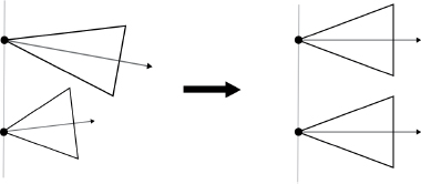
Image rectification is mainly used to calculate disparity maps or to search for the corresponding point in an image which is done using the same line in the other image. It is also used within the context of stereoscopic image production in order to limit vertical parallax between the two images, thereby creating a more comfortable stereoscopic image to look at.

5.4.2. Problems

The principal difficulty in image rectification relates to the fact that there are infinite solutions to the problem. In effect, two perfectly corrected images with a horizontal magnification or skew will remain corrected. This problem is illustrated in Figure 5.6. The aim of image rectification methods is to find a solution that does not alter the original images too much. There are two approaches for solving this problem: image-based methods, focused on explicitly minimizing deformations in the two images, and camera-based methods, which generate corrected images that are compatible with the pinhole camera model. As a result, this second approach is slightly better adapted to correcting images specifically within pinhole cameras.

Figure 5.6. There are infinite solutions to the image correction problem

Finally, a more recent problem relates to how to correct more than two images simultaneously. We will see in section 5.4.5 that this process is possible if the cameras’ centers are aligned. However, if this is not the case, correction will be imperfect or even impossible.

5.4.3. Image-based methods

Since the solution to the rectification problem is not unique, the main aim of rectification methods is to find a solution that does not alter the original images too drastically. The initial motivation of rectification is to generate disparity maps and the scientific community has therefore developed a number of means of minimizing the deformation of processed images without considering the compatibility of the images transformed using camera models. These models are generally linear, i.e. very easy to calculate, and the obtained results are suitable for calculating disparity.

One of the most commonly used methods is that introduced by Hartley [HAR 99]. This method is used within the context of epipolar geometry and involves finding transformations in the two images that place the epipoles at infinity.

This method is fast, easy to implement and available in a large number of computer vision libraries. Its main drawback, however, is its dependence in relation to the distribution of correspondence points on the images which is critical in the last harmonization phase for the second image in relation to the first.

There are also other rectification methods of which the following are the most well known. Robert et al.’s method [ROB 95] seeks transformation that best preserves orthogonality in the image marker as centered coordinates. Loop and Zhang [LOO 99] have proposed a nonlinear model that breaks down the rectification process into an affine transformation followed by a perspective transformation. Finally, Gluckman et al. have researched a transformation that best maintains the bijective character of pixel correspondence from one image to another [GLU 01].

5.4.4. Camera-based methods

Camera-based methods involve finding transformations in images corresponding to those that may occur if we modify the cameras so that they share the same image plane. These methods are nonlinear, i.e. they take longer to calculate than linear methods, but the generated images are equivalent to those that may have been created using decentered lenses combined with an appropriate zoom. In practice, transformations generated in each image are a combination of rotations and a scale, as analyzed in Figure 5.5.

From a more formal perspective, we will consider the two cameras P₁ = K₁ [R₁|– R₁c₁] and P₂ = K₂ [R₂|– R₂c₂], where K is the matrix of the camera’s intrinsic parameters, which includes focal length information, R is a rotation matrix specifying the camera’s direction and c is the camera’s position. The aim of rectification is to find new projection matrices for the cameras so that the cameras share the same image plane. The corresponding transformations in the images are the homographies H₁ and H₂ such that:

The aim of this method is to find the homographies H₁ and H₂ so that the transformed images are rectified. Even an approximate estimation of the matrices K₁ and K₂ will be sufficient to correct the images. The details of this method are further analyzed in [NOZ 11].

5.4.5. Correcting more than two images simultaneously

It is possible to correct more than two images on the condition that the cameras’ centers of projection are aligned. Moreover, epipolar geometry is only defined between two images and is therefore not suitable for correcting more than two images at the same time. The vast majority of rectification methods use epipolar geometry and are therefore not appropriate for correcting several images simultaneously.

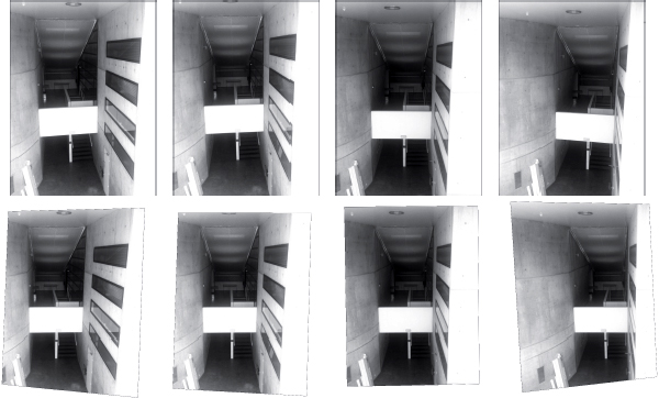
The camera-based method [NOZ 11] presented in section 5.4.4 can be directly adapted to rectify more than two views. Therefore, the problem becomes one of finding the homographies , minimizing the vertical disparity of each correspondence point, no longer between the two images but between all images. Figure 5.7 illustrates a correction of several images.

Figure 5.7. Correction of several images

5.5. Colorimetric considerations in cameras

This section explores the problem of color information raised when filming a scene using a trichromatic red, green, blue (RGB) color camera. Indeed, the relationship between the color perceived when the scene is viewed directly and the digital value acquired by the camera is not straightforward. In addition, we will investigate the concept of color image correction in order to overcome the differences created by the scene’s geometry, given that the scene’s perception is dependent on lighting and angle of view.

To explain these problems, we first analyze several elements of color science and colorimetry that can be used to understand how the digital value of a camera is related to the sensation of perceived color. These elements will also enable us to understand the metrics used to estimate quality as well as cost functions of affiliated inverse problems. Second, we will analyze colorimetric characterization of cameras, i.e. how to connect the sense of color with a digital value. To conclude, we will introduce color corrections in pairs of 3D images.

5.5.1. Elements of applied colorimetry

If we think of the eye as a camera that contains three types of receptors whose spectral sensitivity is known, we can deduce three values that characterize a single point generating the sensation of color. This base simulates a triplet in the large, medium, small (LMS) space, which represents the spectral sensitivities of the photosensitive cells in the eye (see Figure 5.8).

It is important to relate this information to the notion of luminance as defined by the International Commission on Illumination (Commission Internationale de l’Eclairage – CIE) and it is also useful to use the virtual spectral sensitivities defined by the CIE for a given angle of view, i.e. 2° or 10° (Figure 5.8). These data define the space XYZ, characterizing the color of an object in a scene, according to its reflection properties R(λ) (the quantity of energy reflected by the object in relation to wavelength) and a given light level I (λ) (the quantity of energy reaching an object in relation to wavelength).

To evaluate the difference between two similar colors, the CIE recommends working within a more perceptual space where the Euclidean distance is less representative of the perceived difference than the physical projection space XYZ, i.e. CIELAB. The distinctive feature of a typical pseudo-perceptual space is a nonlinear transformation (pseudo-logarithmic, see Weber–Fechner’s law) of the values XYZ weighted by a so-called reference white (X_n, Y_n, Z_n), representing the illumination in the scene. Note that a colorimetric system, which organizes colors in relation to each other, such as the “Munsell” system, is also pseudo-perceptual but is not a colorimetric space in itself.

Figure 5.8. Spectral sensitivities of cones (LMS, normalized by M), of primaries defined by the International Commission on Illumination (CIE), and of a camera r, g, b (Sinarback 54 Camera [DAY 03])

In CIELAB, the perceptual difference between two similar colors C₁ and C₂ can be expressed by using the Euclidean distance, denoted as . The subscript 76 refers to the formulation’s year of acceptance, and similarly we will use 94, CMC, 00 among others for distinction between metrics. Euclidean distance being an approximation, several improvements based on experimental data have been proposed, giving rise to non-Euclidean metrics that better fit our own perception and whose principal feature is that they weight the Euclidean distance for strongly chromatic colors, where the perceived difference is less sensitive to small variations.

In particular, incorporates a weight function for hue and chromaticity while , in addition to modifying specific parameters present in , adds an intermediary crossing term between chroma and hue as well as a weight on the axis a*, which affects similar colors within the chromatic axis where very small signal variations can be perceived.

We will not analyze the specification of a color in terms of luminance/brightness, hue and saturation, or the appearance of color or the different systems such as Atlas or Espace that predict the appearance of color or a physical signal. However, there is a broad literature on this subject, particularly in relation to CIE standards for a more extensive formulation of the material analyzed previously [CIE 01, CIE 04], Wyszecki and Stiles’ comprehensive study of modern colorimetry [WYS 00] or Fairchild’s excellent investigation of the appearance of color [FAI 98], among others.

The connection with capturing a scene via an RGB color camera becomes apparent when we analyze spectral sensitivities in cameras (see Figure 5.8). If the spectral sensitivities of a camera can be defined by a linear combination of the eye’s spectral sensitivities, our camera is said to be colorimetric (Luther-Yves condition). However, physical and material constraints mean that this condition is often not respected, and the three RGB values provided by a camera are not directly representative of the perceived color. The quality index of a set of filters defined by Vora and Trusell [VOR 93] evaluates the difference in sensitivity between the camera and the human eye via the angle between the space defined by the camera’s filter and the space formed by the sensitivity of the human visual system. Different quality indicators can be used and have been compared by Hung [HUN 00]. To conclude this brief overview, we should highlight two fundamental implications. On the one hand, the integration of the same spectral signal by different systems will not give the same result (the value representing color and the corresponding digital value after acquisition will be different) and, on the other hand, the integration of two different signals may give similar values between two systems and therefore create confusion (difference of metamerism). The other significant aspect of this section is that we have defined a space and metric to evaluate the difference between two colors. In the next section, we will explain colorimetric characterization/calibration of a color camera.

5.5.2. Colorimetric calibration in cameras

Colorimetric characterization of RGB trichromatic cameras is designed to establish the relationship between the digital value acquired and a value representing color. The calculation of digital values from a color value is called “model” and an “inverse model” relates to a color value taken from digital values. Different methods have been proposed in the literature. However, we will focus on a purely conceptual study. There is an extensive body of literature available on this subject for further information.

The characterization of a camera is generally carried out in two stages: a linearization stage and a colorimetric transformation stage.

The following discussion is primarily inspired by the excellent article by Barnard and Funt [BAR 02] as well as that by Cheung et al. [CHE 05]. We also highly recommend Gaurav Sharma’s book [SHA 97] for a more encompassing view of colorimetric characterization as well as other problems related to color imaging. First, we will define the acquisition model and use this to define the spectral sensitivities in a camera, i.e., the characterization in the proper sense of the term. Second, we will analyze the practical aspect by focusing on application, i.e. how to obtain a colorimetric value from digital values given by the camera. We will use the model previously defined for the human eye and apply it to cameras.

We suppose that the sensor’s nonlinearity is independent of wavelength. The effects of “vignetting” and other geometric effects are not included, but can be integrated into the model either in F^(k) or in S^(k), if we consider them as independent of wavelength (see the following equations). Equally, the effects of diaphragm opening, focal and acquisition time are fixed and appropriate. In general, a relative characterization is enough to guarantee color information, but it is also possible to find the absolute values by following the propositions of Martinez-Verdu et al. [MAR 03] or Debevec and Malik [DEB 97].

Given L(λ), the radiance of the scene is the convolution over a set of wavelenghts (λ) of the light source illuminationg the scene, I(λ) and of the reflectance properties of the objects composing the scene, R(λ). Given, the spectral sensitivities of the sensor S^(k)(λ), and given ν^(k), the value given by the sensor in answer to L(λ) for a channel k, typically k ∈ R, G, B, we have:

[5.1]

where F^(k) is a linearization function and ρ^(k) is the linearized value (the camera’s response). F^(k) is typically a correction of the camera’s gamma and offset.

The measure and the representation of this information is usually discrete, and L(λ) and S(λ) become the vectors L and S. Therefore, equation [5.1] becomes:

[5.2]

The characterization of a camera therefore requires estimating F^(k) and S^(k).

5.5.2.1. Estimation of F^(k) and S^(k)

If we suppose that F^(k) is independent of wavelength, we can estimate it by stimulating the camera with a light source, which has its intensity varied (with different density filters or even by taking the light source further away). The data can be interpolated or approximated using a smooth function and a “look-up table” (LUT) can be created. In general, the camera is considered to be linear throughout most of the domain but for the weakest intensity values we often see a nonlinearity, which must be accounted for by a more precise characterization. Regardless of this, however, this hypothesis must be verified in order for it to be reliable. Often a gamma correction is applied by the constructor, by default, to the camera data to bring the camera’s RGB values closer to the sRGB standard and the inverse of this correction must be applied.

In order to obtain S^(k), the simplest method to use conceptually is a monochromator, i.e. to stimulate the camera using signals in a very narrow bandwidth. This approach requires expensive material and is not commonly used in practice outside of laboratories.

Other methods have also been developed in order to overcome this material constraint. The general approach consists of evaluating F^(k), and then measuring a finite number of spectra (generally of a smaller size than the discretization required to reconstruct a spectrum) and the corresponding values after acquisition by the camera. If we consider r^(k), a vector whose elements are the responses of the linearized camera, L a matrix whose lines are samples of known spectrums, we can write using equation [5.2]:

[5.3]

We therefore find S^(k) by finding a solution to the linear system above. However, the problem is said to be hill-posed, which means that the amount of data is often too small to strictly solve the equation. When L contains enough information, we have a situation similar to that found with a monochromator. By directly calculating the pseudo-inverse of L using a reduced number of measurements, the result is highly unstable, particularly because it is the noise that is mostly adjusted. Therefore, the estimation of the sensor’s sensitivity curves shows a number of peaks and negative values.

Various methods providing acceptable results include finding an approximate solution to the problem rather than an exact solution. This solution is subject to a number of constraints and uses a number of different methods and tools. The constraints typically include the positivity of values, ensuring that the curves are smooth, analyzing their modality (the sensors’ responses are often uni- or bimodal, not in the strict mathematical sense but in an overall sense), limiting the maximum error tolerated, etc. Various methods may include second derivative analysis, Wiener methods, using a combination of Fourier series or the addition of regularization terms. For further information on the advantages, disadvantages and implementation of such methods, see [BAR 02, FIN 98, JOH 96, SHA 96, SHA 97].

5.5.2.2. In practice

Beyond the physical aspects, in practice, it may be sufficient to have a mapping of a data set taken from a camera (in an RGB space specific to the camera) to a space representative of color perception, such as XYZ or CIELAB. If we reuse a linear model, we have:

[5.4]

where υ is a vector containing colorimetric values, c is a vector containing data from the camera and M is a transformation matrix. If the Luther-Yves conditions are respected, M is a matrix with a size of 3 × 3. If this is not the case, matrix M must be of a greater size (3 × n) and c must contain values of cross-components, typically m = 10, including the terms R, G, B, RG, RB, BG, R², G², B² and an offset term. The matrix M is typically adjusted using a least squares method based on a training data set (consisting of known values obtained from a color chart with known reflectances), such as the X-rite Colorchecker Classic, depending on the function to be minimized. This function is based on the perceived difference between the reference values and the values calculated by the model ( or similar). Similar to adjusting polynomials, this transformation can be achieved using networks of neurons or different interpolation techniques. In particular, good results have been obtained using radial basis functions (RBF) with polyharmonic kernels [THO 11]. There is an abundance of literature on this subject, beyond the scope of this chapter [CHE 02, CHE 04, CHE 05, HON 01, JOH 96, SHA 00].

These methods are evaluated based on a statistically significant set of known reflectances, independent from the data used to establish the model. The difference between the actual colors and the evaluated colors is measured using one of the metrics mentioned above. Significant values may include average error, variance and maximum error. The 90th or 95th percentiles also provide good indications. It is often useful to know where in the color space the model shows the least amount of precision, and visualizations can therefore provide a good indication of the model’s behavior.

To conclude, while assuming the response in intensity to be linear or corrected for its nonlinearity, there are three main possibilities to consider:

The characterization data are normally stored within a standard International Color Consortium (ICC) file in order to be used by a color management system.

5.6. Conclusion

When capturing a scene using two cameras, the geometric correspondence between the two images is not evident for reasons such as the distance between the object and two or multiple cameras. Equally, the correspondence between the color of one object in pictures taken by several cameras is far from obvious for various reasons. Reasons for this include:

These considerations and adequate solutions can also be applied to capture a scene using multiple cameras as well as taking several images of the same scene using the same camera for a 3D effect or reconstruction, and even to recreate a panoramic view based on several images. It is therefore necessary to obtain correspondence between various parts in the scene and to define a transformation, which can standardize the sensation of color; a “color correction”, also known as “color mapping”.

5.7. Bibliography

[BAR 02] BARNARD K., FUNT B., “Camera characterization for color research”, Color Research & Application, vol. 27, no. 3, pp. 152–163, 2002.

[CHE 02] CHEUNG V., WESTLAND S., “Color camera characterisation using artificial neural networks”, 10th Color and Imaging Conference (CIC’10), 2002, Scottsdale, Arizona, pp. 117 –120, 12–20 12–15 November 2002.

[CHE 04] CHEUNG V., WESTLAND S., CONNAH D., et al., “A comparative study of the characterisation of colour cameras by means of neural networks and polynomial transforms”, Coloration Technology, vol. 120, no. 1, pp. 19–25, 2004.

[CHE 05] CHEUNG V., WESTLAND S., LI C., et al., “Characterization of trichromatic color cameras by using a new multispectral imaging technique”, Journal of the Optical Society of America A, vol. 22, no. 7, pp. 1231–1240, July 2005.

[CIE 01] CIE, 142-2001, Improvement to Industrial Colour-Difference Evaluation, Commission Internationale de l’Eclairage, 2001.

[CIE 04] CIE, 015:2004, Colorimetry, 3rd ed., Commission Internationale de l’Eclairage, 2004.

[DAY 03] DAY D.C., Spectral sensitivities of the sinarback 54 camera, Technical report, Spectral Color Imaging Laboratory Group Munsell Color Science Laboratory Chester F. Carlson Center for Imaging Science Rochester Institute of Technology, February 2003.

[DEB 97] DEBEVEC P.E., MALIK J., “Recovering high dynamic range radiance maps from photographs”, Proceedings of the 24th Annual Conference on Computer Graphics and Interactive Techniques, SIGGRAPH ’97, ACM Press/Addison-Wesley Publishing Co., New York, NY, pp. 369–378, 1997.

[DEV 01] DEVERNAY F., FAUGERAS O., “Straight lines have to be straight: automatic calibration and removal of distortion from scenes of structured environments”, Machine Vision and Application, vol. 13, no. 1, pp. 14–24, August 2001.

[FAI 98] FAIRCHILD M.D., Color Appearance Models, Addison-Wesley, Reading, MA, 1998.

[FIN 98] FINLAYSON G.D., HORDLEY S., HUBELL P.M., “Recovering device sensitivities using quadratic programming”, IS&T and SID’s Color Imaging Conference (CIC’6), Scottsdale, Arizona, 17–20 November 1998.

[GLU 01] GLUCKMAN J., NAYAR S.K., “Rectifying transformations that minimize resampling effects”, IEEE Computer Society Conference on Computer Vision and Pattern Recognition, Scottsdale, Arizona, vol. 1, IEEE Computer Society, pp. 111–117, 7–10 November 2001.

[HAR 99] HARTLEY R.I., “Theory and practice of projective rectification”, International Journal of Computer Vision, vol. 35, no. 2, pp. 115–127, 1999.

[HAR 04] HARTLEY R.I., ZISSERMAN A., Multiple View Geometry in Computer Vision, 2nd ed., Cambridge University Press, 2004.

[HON 01] HONG G., LUO M.R., RHODES P.A., “A study of digital camera colorimetric characterization based on polynomial modeling”, Color Research & Application, vol. 26, no. 1, pp. 76–84, 2001.

[HUN 00] HUNG P.-C., “Comparison of camera quality indexes”, 8th Color and Imaging Conference (CIC’8), 2000, Scottsdale, Arizona, pp. 167–171, 7–10 November 2000.

[JOH 96] JOHNSON T., “Methods for characterizing colour scanners and digital cameras”, Displays, vol. 16, no. 4, pp. 183–191, 1996.

[LOO 99] LOOP C., ZHANG Z., “Computing rectifying homographies for stereo vision”, Computer Vision and Pattern Recognition, vol. 1, pp. 1125–1131, 1999.

[MAR 03] MARTÍNEZ-VERDU F., PUJOL J., VILASECA M., et al., “Characterization of a digital camera as an absolute tristimulus colorimeter”, in MARTÍNEZ-VERD U.F., PUJOL J., CAPILLA P. (eds), Imaging Science and Technology, vol. 47, no. 4, pp. 279–295, 2003.

[NIS 04] NISTÉR D., “An efficient solution to the five-point relative pose problem”, IEEE Transactions on Pattern Analysis and Machine Intelligence, vol. 26, no. 6, pp. 756–777, June 2004.

[NOZ 11] NOZICK V., “Multiple view image rectification”, Proceeding of IEEE-ISAS 2011, International Symposium on Access Spaces, Yokohama, Japan, pp. 277–282, 17–19 June 2011.

[ROB 95] ROBERT L., ZELLER C., FAUGERAS O., et al., Applications of non-metric vision to some visually guided robotics tasks, Report no. RR-2584, INRIA, June 1995.

[SHA 96] SHARMA G., TRUSSELL H., “Set theoretic estimation in color scanner characterization”, Journal of Electronic Imaging, vol. 5, no. 4, pp. 479–489, 1996.

[SHA 97] SHARMA G., TRUSSELL H., “Digital color imaging”, IEEE Transactions on Image Processing, vol. 6, no. 7, pp. 901–932, 1997.

[SHA 00] SHARMA G., “Targetless scanner color calibration”, Journal of Imaging Science and Technology, vol. 44, no. 4, pp. 301–307, 2000.

[STR 05] STRAND R., HAYMAN E., “Correcting radial distortion by circle fitting”, Proceedings of the British Machine Vision Conference, BMVA Press, pp. 9.1–9.10, 2005.

[THO 11] THOMAS J.-B., BOUST C., “Colorimetric characterization of a positive film scanner using an extremely reduced training data set”, 19th Color and Imaging Conference (CIC’19), 2011, San Jose, California, 7–11 November 2011.

[TRI 00] TRIGGS B., MCLAUCHLAN P., HARTLEY R.I., et al., “Bundle adjustment – a modern synthesis”, Vision Algorithms: Theory and Practice, vol. 1883, pp. 153–177, 2000.

[VOR 93] VORA P.L., TRUSSELL H.J., “Measure of goodness of a set of color-scanning filters”, Journal of the Optical Society of America A, vol. 10, no. 7, pp. 1499–1508, July 1993.

[WYS 00] WYSZECKI G., STILES W.S., Color Science: Concepts and Methods, Quantitative Data and Formulae (Wiley Series in Pure and Applied Optics), 2nd ed. Wiley-Interscience, 2000.

[ZHA 00] ZHANG Z., “A flexible new technique for camera calibration”, IEEE Transactions on Pattern Analysis and Machine Intelligence, vol. 22, no. 11, pp. 1330–1334, November 2000.

Chapter written by Vincent NOZICK and Jean-Baptiste THOMAS.