CHAPTER 9

Statistical Properties and Tests of Efficient Frontier Portfolios

C J Adcock

Sheffield University Management School, Sheffield, UK

INTRODUCTION

The standard theory of portfolio selection due to Markowitz (1952) makes an implicit assumption that asset returns follow a multivariate normal distribution. The original concept of minimizing portfolio variance subject to achieving a target expected return is equivalent to assuming that investors maximize the expected value of a utility function that is quadratic in portfolio returns. Stein's lemma (1981) means that Markowitz's efficient frontier arises under normally distributed returns for any suitable utility function, subject only to relatively undemanding regularity conditions. Recent developments of the lemma (e.g., Liu, 1994; Landsman and Nešlehová, 2008) show that the efficient frontier arises under multivariate probability distributions that are members of the elliptically symmetric class (Fang, Kotz and Ng, 1990). There is a direct extension to a mean-variance-skewness efficient surface for some classes of multivariate distributions that incorporate asymmetry (Adcock, 2014a).

The literature that addresses the theory and application of Markowitzian portfolio selection is very large. Much of this published work assumes that the parameters of the underlying distributions, most commonly the vector of expected returns and the covariance matrix, are known. In reality, they are not known and all practical portfolio selection is based on estimated parameters. There is also often at least an implicit assumption made about the appropriate probability distribution. Practitioners, in particular, are well aware that the effect of estimation error is almost always to ensure that the ex post performance of a portfolio is inferior to that expected ex ante. Notwithstanding that the effects of estimation error can be serious, the literature that deals formally with the effect of estimated parameters is still relatively small. Furthermore, the number of papers in the area that can be regarded as well-known is even smaller.

Investigations of the sensitivity of portfolio performance are due to the well-known works of Best and Grauer (1991) and Chopra and Ziemba (1993). The latter paper, in particular, is considered by some to be the source of the rule of thumb that errors in the estimated expected return are 10 times more serious than errors in the estimate of variance. There is an early monograph that addresses parameter uncertainty; see Bawa, Brown, and Klein (1979). There are also works that provide tests of the efficiency (in Markowitz's sense) of a given portfolio. These works include papers by Jobson and Korkie (1980), Gibbons, Ross and Shanken (1989), Britten-Jones (1999), and Huberman and Kandel (1987), among others. Huberman and Kandel, in particular, present likelihood ratio type tests for efficiency, thus continuing a theme of research due to Ross (1980) and Kandel (1983, 1984). There is a recent survey in Sentana (2009).

In addition to these works, there is a more recent stream of literature that is concerned with the effect of estimated parameters on the properties of the weights of an efficient portfolio and on the components of the equation of the efficient frontier itself. Most of this literature considers the case where the vector time series of asset returns is IID normally distributed and the only restriction in portfolio selection is the budget constraint. Even under the IID normal and budget constraint assumptions, the majority of results that have appeared in recent literature are complicated mathematically. As several authors point out, actual computations are today relatively easy to undertake because of the wide availability of suitable software. However, understanding the derivations in sufficient detail to allow a reader to make further advances is a more demanding task. This surely acts to inhibit use of these methods, if not further technical development, by researchers.

It is helpful to classify the areas in which new methods have been developed. Inevitably, there is some overlap, but nonetheless it is useful to consider three areas: First, there are papers that are concerned with the properties of the vector of portfolio weights. At a general level, there are three distinct sets of weights to consider that correspond to different maximization criteria. These are: (1) the tangency portfolio, which arises when a position in the risk-free asset is allowed; (2) the maximum Sharpe ratio or market portfolio, which is the point on the efficient frontier that is the tangent to the risk-free rate; (3) the portfolio that arises from Markowitz's original criterion or from maximizing the expected value of a quadratic utility function. Second, there are papers that present results concerning the distribution of the three scalar parameters that determine the location, scale, and slope of the equation of the efficient frontier. As is well known, there are analytic expressions for these in terms of the mean vector and covariance matrix (see Merton, 1972). The majority of the extant literature in the area is concerned with these two sets, both of which address the behavior of a portfolio ex ante. Third, there is a small literature that is concerned with ex post performance.

Even though the total number of papers that address the effect of parameter uncertainty is small, the technical nature of the subject means that it is impractical to consider all three areas of research in a single article. This paper is therefore concerned with the first topic—namely, the distribution of portfolio weights. The second topic, the properties of the parameters of the efficient frontier, is described in Adcock (2014b). The third area is discussed briefly in the conclusions to this article. The article contains a summary of the state of the art and presents some new results. The article is not a complete survey of all works in the area. In the manner of Smith (1976) and quoting Adcock (1997), “Ideas are interpreted from a personal point of view and no attempt is made to be completely comprehensive … any review could only address a subset of approaches and application areas.” Furthermore and quoting Smith (1976) himself, “No review can ever replace a thorough reading of a fundamental paper since what is left out is often just as important as what is included.”

As the title indicates, the following sections present statistical tests for portfolio weights. As is clear from the literature, the probability distribution of portfolio weights is often confounded by nuisance parameters. Development of suitable test statistics thus requires either approximations or perhaps some ingenuity. However, as is shown next, it is possible to develop likelihood ratio tests, thus continuing the research first reported by Ross (1980) and Kandel (1983, 1984). These avoid the nuisance parameters and the difficulties of using exact distributions. Likelihood ratio tests employ a standard distribution, but rely on asymptotics for their properties. They may therefore be unsuitable for portfolio selection in which only a small number of observations are used. They also depend on the IID normal assumption, which implies that they are more likely to be useful for low-frequency returns, when it is possible to rely to an extent on the central limit theorem. However, given that even IID normality leads to mathematically complex results, the case for a simple approach, which depends on a standard distribution, is a strong one.

The structure is of this chapter is as follows. The first section below presents notation and summarizes the standard formulae for portfolio weights. This is followed by the main methodological content of the article. This contains both the review of relevant literature and the presentation of new tests. To contain the length of the article, technical details of development of the tests are omitted, but are in Adcock (2014b). The penultimate section presents an empirical study in which the results are exemplified. The last section contains concluding remarks and a short description of outstanding research issues. Notation not explicitly defined in the next section is that in common use.

NOTATION AND SETUP

The notation used in this article is that in widespread use in this area of financial economics. It follows Okhrin and Schmid (2006) and related papers, such as Bodnar and Schmid (2008a, 2008b), Adcock (2013), and several others.

It is assumed that there are n assets and observations for T time periods. The time subscript t is omitted unless needed explicitly. The n-vector of asset returns is denoted by R. It is assumed that the vector time series is IID multivariate normal, N(μ, Σ) in the usual notation, and that the covariance matrix Σ is nonsingular. The inverse of the covariance matrix is denoted by Ψ. The n-vector of portfolio weights and the budget constraint are denoted by w and 1 respectively. Portfolio return w^TR is denoted by R_p. Given the assumptions, this has the normal distribution N(μ_p, ), with μ_p = w^Tμ and = w^TΣw. The risk free rate is R_f. Excess returns are denoted by and with corresponding notation for expected returns. Parameter estimates are denoted with the symbol ^, for example . In the results described below it should be assumed that T is always big enough for relevant moments to exist. Restrictions on both T and n will be clear from the context. It is assumed that parameters are estimated by the sample moments, that is

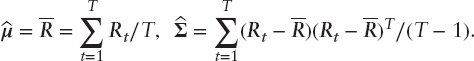
In this case and has the independent Wishart distribution W_n(q, Σ/q) with q = T − 1.

The standard approach to portfolio selection is to maximize the expected value of the quadratic utility function

where θ ≥ 0 measures the investor's appetite for risk. Expectations are taken over the distribution of R_p in the standard frequentist manner, assuming that the parameters are given. As noted in the introduction, a consequence of Stein's lemma (Stein, 1981), is that under normally distributed returns, the quadratic utility function may be used without loss of generality; subject to regularity conditions all utility functions will lead to Markowitz's efficient frontier. The objective function to be maximized is

subject to the budget constraint w^T1 = 1. The solution is

where

The vector w₀ is the minimum variance portfolio, and w₁ is a self-financing portfolio. The expected return and variance of the portfolio are respectively

where the standard constants are

Note that these are not quite the same as the standard constants as defined in Merton (1972) but are more convenient for the current purpose.

In this formulation, the parameter θ is given even when μ and Σ are replaced by estimates. An important variation is to specify a target expected return τ. In this case θ = (τ − α₀)/α₁, which then also becomes an estimated value. As next described, this can make a material difference to the distribution of the estimated portfolio weights. A third formulation is to maximize the Sharpe ratio. In this case, the vector of portfolio weights is

The final formulation is to assume the availability of the risk-free rate. An amount w^T1 is invested in risky assets and 1 − w^T1 in the risk-free asset. This setup generates the security market line, which is the tangent to the efficient frontier. The vector of portfolio weights is

As above, a variation is to specify a target expected return τ. In this case, . Consistent with these notations, the vectors of estimated portfolio weights are denoted where the subscript takes values θ, 0, S and T and the above estimators of μ and Σ are used. Note that the notation T plays three roles in the paper, but no confusion arises.

DISTRIBUTION OF PORTFOLIO WEIGHTS

The substantial paper by Okhrin and Schmid (2006), O&S henceforth, presents expressions for the vector of expected values of the portfolio weights and for their covariance matrices. These are accompanied by numerous results for the portfolio selection approaches described previously. This section contains a summary of the results in O&S as well as results from other authors. New results, which overcome some of the difficulties posed by the nuisance parameters problems referred to in the introduction, are from Adcock (2014b). The results presented are illustrated with an empirical study, which is reported in the next section.

Tangency Portfolio with One Risky Asset

O&S consider the tangency portfolio, with estimated weights

Since this depends on risk appetite θ, in what follows it is assumed that θ = 1. As O&S note, the scalar case in which there is one risky asset is of importance. This is because it is relevant to the basic asset allocation decision between risky and nonrisky assets. In this case,

with and independently distributed as, respectively

The mean and variance of are respectively

These results illustrate that is a biased estimator of w_T and that the variance may be materially affected if the tangency weight is of comparable magnitude to 1/σ or larger. The probability density function of may be obtained by standard methods. In the notation of this article, it is

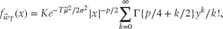
where Γ(υ) with υ > 0 is Euler's gamma function and

This expression is proportional to the hypergeometric function ₁F₁. O&S show that it may also be expressed as the difference of two such functions and note that it may be computed using routines that are readily available. The probability density function provides an illustration of the fact, already noted in the introduction, that the statistical properties of the efficient frontier are confounded by the nuisance parameter, in this case σ. Inference is therefore complicated, and within the standard frequentist approach it is necessary to consider approximations. A practical test of the null hypothesis H₀ : w_T = against both one- and two-sided alternatives is provided by the statistic

This is assumed to have a standard normal distribution. The accuracy of this test procedure may be computed as follows. First note that, conditional on the estimated variance

where . Hence,

where f_U() is the probability density function of U and Φ(x) is the standard normal distribution function evaluated at x. This integral may be used to compute the exact distribution function of and hence evaluate the accuracy of the test statistic Z_T. Since the probability density function of U has a single mode and vanishes at the end points, this integral may be may computed to any desired degree of accuracy using the trapezoidal rule. For some exercises in portfolio selection, the sample size T will be large. In such cases, the test is supported by a result reported in Adcock (2014b), which shows that the asymptotic distribution of Z_T is N(0, 1). An alternative approach is to use a likelihood ratio test. For this, the null hypothesis is that a given investment weight is a tangency portfolio, that is

The alternate hypothesis is that there is no restriction on either μ or σ². Under the null hypothesis, the maximum likelihood estimator (MLE) of σ², which is now the sole free parameter, is

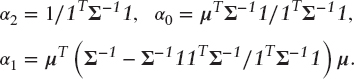
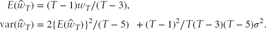
The resulting likelihood ratio test statistic, which is computed in the usual way, is distributed as under the null hypothesis. The sensitivity of estimates of w_T may be investigated using the exact or approximate distributions reported above. The normal approximation, for example, may be used to compute confidence limits for w_T. It is also interesting to note that the partial derivatives of w_T with respect to μ and σ² are

and that the ratio of these is equal to −w⁻¹. Thus, for small values of the absolute value of w_T, the weight is more sensitive to changes in w_T itself. For large values, the opposite is true.

Tangency Portfolio with n Risky Assets

For the general case with n risky assets, the estimated weights of the tangency portfolio (and with θ = 1) are

O&S opine that it is difficult to generalize the results from the case n = 1. To some extent this is true, although there are recent results in Bodnar and Okhrin (2011). The expected value of is however straightforward to compute. Using the independence property of and , and a result from Muirhead (1982, p. 97), it follows that

Using Siskind (1972), who reprises an earlier result from Das Gupta (1968), the covariance matrix is

with the constants r_i given by

The distribution of is not straightforward to compute and would in any case depend on nuisance parameters. In the spirit of the results for the univariate case, the null hypothesis H₀ : w_T = against suitable alternatives can be tested by the statistic

and comparing the computed value with percentage points of the Chi-squared distribution with n degrees of freedom. A procedure that avoids the nuisance parameter more formally is based on the likelihood ratio test. For a given portfolio w_T the null hypothesis is . The MLEs of and Σ may be computed numerically and the resulting likelihood ratio test also has n degrees of freedom. As noted in the introduction, details of this and other likelihood ratio tests are in Adcock (2014b). A variation on the tangency portfolio is in Ross (1980). In this, the expected return is specified to be equal to τ, in which case the degree of risk is estimated as .

Maximum Sharpe Ratio Portfolio

In Proposition 2, O&S show that the moments of the elements of , the vector of estimated weights that maximizes the Sharpe ratio, do not exist. Additional results are reported in Bodnar and Schmid (2008a) concerning the distribution of the estimated return and variance of the maximum Sharpe ratio portfolio. As they report, moments of order one and, hence, greater do not exist for the estimated return. For the estimated variance, moments of order greater than one half do not exist. These results are for estimated ex ante returns. There is also a related result in Proposition 8 of Adcock (2013), which is concerned with ex post properties of efficient portfolios.

The implication of these results is both serious and noteworthy. Maximizing the Sharpe ratio is an important component of finance theory because of its connections to the CAPM and to the market portfolio. The Sharpe ratio is a widely used practical measure of portfolio performance. That the estimated weights and return have undefined moments implies that a maximum Sharpe ratio portfolio may be a dangerous point on the efficient frontier both ex ante and ex post. It is interesting, however, to note that the paper by Jobson and Korkie (1980) presents tests for the maximum Sharpe ratio portfolio based on the delta method. These thus avoid problems of nonexistence of moments. They also serve to remind that the assumption of normality is of course a convenient mathematical fiction. It seems clear, though, that it is safe to say the maximum Sharpe ratio portfolios are likely to be volatile in the presence of estimation error. This is supported by the study by Britten-Jones (1999), who presents a regression-based test of maximum Sharpe ratio portfolios. He reports the results of a study of 11 international stock indices and writes, “The sampling error in the weights of a global efficient portfolio is large.”

As reported in O&S, the probability distribution of the weights involves nuisance parameters. Notwithstanding the properties reported in the preceding paragraphs, a likelihood ratio test is available. For a given portfolio with weights w_S the null hypothesis is

As shown earlier, the MLEs of and Σ might be computed numerically, and the resulting likelihood ratio test has n degrees of freedom. Bodnar and Okhrin (2011) present a test for a linear combination of weights in the maximum Sharpe ratio portfolio based on Student's t-distribution. They also describe more general tests that are based on expression for the distribution of . As they note, these are complicated to evaluate in general.

Expected Utility with Set Risk Appetite

Using the notation defined in the previous section, in Theorem 1 of O&S the expected value of is

and the corresponding covariance matrix is

where

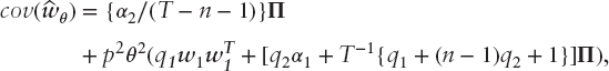
As O&S remark, the estimated weights are biased estimators of the population values. The biases may be removed, but at the expense of an increase in variability. However, an alternative interpretation is that, after allowing for the effect of estimation error, the weights are unbiased for a point on the efficient frontier corresponding to the higher risk appetite pθ. Thus, an investor may construct a portfolio with risk appetite θ in an expected value sense by using p⁻¹θ. A more worrying aspect is that if the number of observations is not large relative to the number of assets, the effective point on the frontier may be materially different from that intended. For example, an asset allocation portfolio with ten assets based on a sample of 36 months results in p = 1.4, loosely speaking, 40 percent further up the frontier than intended.

In their Theorem 1, O&S show that the vector of weights has an asymptotic multivariate normal distribution. Indeed for large T the covariance matrix is well approximated by

This expression demonstrates that the penalty of uncertainty in the covariance matrix is substantial, at least in algebraic terms. Assume that the covariance matrix is given and that only the vector of expected returns in estimated. In this case, the covariance matrix of is θ²Π/T. It may also be noted that the two components of , the minimum variance and self-financing portfolios, are uncorrelated.

Bodnar and Schmid (2008b) provide the distribution for affine transformations of , the estimated minimum variance portfolio. This is a multivariate Student distribution, but is confounded by nuisance parameters. They provide a test statistic, in which the nuisance parameters are replaced by their estimators. This is similar in spirit to the tests reported in the two previous sections. Under suitable null hypotheses this statistic has an F-distribution. Computations of power require integration of the product of an F density with the hypergeometric function ₂F₁.

For a likelihood ratio test, the null hypothesis is

The resulting likelihood ratio test has 2n degrees of freedom. The test for the minimum variance portfolio omits the second component and has n degrees of freedom. This may be contrasted with the test based on regression that is reported in Gibbons, Ross, and Shanken (1989) and which results in a F-test based on n and T − n − 1 degrees of freedom. There are also related tests in Huberman and Kandel (1987) that are concerned with mean-variance spanning and in Jobson and Korkie (1989).

Expected Utility Portfolio with Expected Return Target

A common extension to the expected utility approach is to specify an expected return target τ. In this case, risk appetite is given by

and the portfolio weights are denoted by w_τ. Computation of portfolio weights, expected return and variance then employs in which α_0,1 are replaced by their estimated values. Kandel (1984) presents a likelihood ratio test. A stochastic representation of the distribution of the weights is reported in Kan and Smith (2008), which is another substantial paper in this area of financial economics. They use this to derive the expected value and covariance matrix. Their results provide a clear illustration of the complexity of this area. The expected value of the weights is

where β is a nonnegative constant defined in their equation (39). In the notation of this paper it is

The covariance matrix is reported in equations (56) to (58) of Kan and Smith (2008). To simplify the presentation here, the following notation is used

along with a random variable W, which is defined as

where U and V are independent random variables distributed as and , respectively. The notation denotes a noncentral Chi-squared variable with υ degrees of freedom and noncentrality parameter λ and follows the definitions in Johnson and Kotz (1970, p. 132). Using this notation, the covariance matrix is

where

and

In Proposition 1, Kan and Smith (2008) present results for the distribution of the estimated values of the standard constants. In the present notation, these are as follows:

where Q, R, and Z are independent random variables distributed as follows:

In this notation, the estimated risk appetite is

As shown in Adcock (2014b), the mean and variance of are

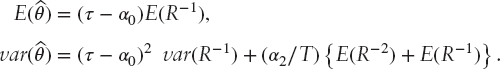
It is possible to compute the mean and variance analytically for the unusual case in which α₁ = 0. For other cases, the mean and variance of R⁻¹ are evaluated numerically. The distribution function may be written as

where f_R(.) denotes the probability density function of R. As above, this integral may be evaluated using the trapezoidal rule. In the following section, it is shown that, at least for the assets considered, confidence limits for θ are wide. That is, it is possible for a portfolio to be at a point on the efficient frontier that is materially different from that expected. This is further discussed in the concluding section.

EMPIRICAL STUDY

This section contains examples of tests described in the previous section. It is based on returns computed from 608 weekly values of 11 FTSE indices from June 10, 2000, to January 28, 2012. These indices are chosen for illustrative purposes to exemplify the tests. These indices were also used as exemplars in Adcock et al. (2012). The text in this paragraph and Tables 9.1 and 9.2 are taken with minor modifications from that paper. Weekly returns were computed by taking logarithms. The means, variances, and covariances were estimated using the sample data. Descriptive statistics for the 11 indices are shown in Table 9.1. This table indicates that the weekly returns on these indices are not normally distributed. The risk-free rate is taken to be equal to zero.

Table 9.2 shows variances, covariances, and correlations for returns on the indices. Covariances are shown above the leading diagonal and correlations below.

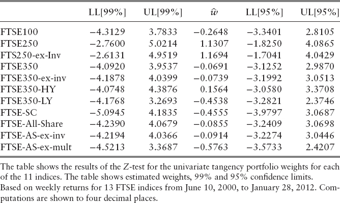
Table 9.3 shows the results of the Z-test for the univariate tangency portfolio weights for each of the 11 indices. Table 9.3 shows that estimated weight, together with 99 percent and 95 percent confidence limits. As the table clearly demonstrates, the limits are wide.

Panel (1) of Table 9.4 shows the likelihood ratio test probabilities for univariate tangency weights. The value of the weight under the null hypothesis is shown at the head of each column. The results in Panel (1) confirm the results in Table 9.3, namely that the univariate tangency portfolio weights are volatile. For example the absolute value of the tangency weight for the FTSE100 index has to be greater than 2.5 before the null hypothesis is rejected. Panel (2) of Table 9.4 shows the p-values for the corresponding Z-test. As Table 9.4 shows, these are very similar to the corresponding cells in panel (1) and, when displayed to four decimal places, are the same in many cases.

Table 9.5 shows lower and upper 99 percent confidence limits for the FTSE100 index for a range of values of expected return and variance. In the table, these ranges are shown as percentages of the sample estimates used in preceding tables, as reported in Table 9.1. The columns of Table 9.5 show variation in the expected return and rows show variation in variance. As the table shows, the confidence limits are relatively robust to changes in expected return, but not to changes in variance. The two numbers reported in boldface type correspond to the values shown for the FTSE100 in Table 9.3. The corresponding tables for the other indices are available on request.

Table 9.6 shows simultaneous confidence intervals for each of the weights in the (multivariate) tangency portfolio based on Scheffé's method (Scheffé 1959, p. 406). Also shown in the table are the estimated tangency portfolio weights. As the table makes clear, the weights are very different from those estimated using univariate methods. This is due to the high sample correlations between the returns on these FTSE indices as shown in Table 9.2. The multivariate confidence limits are also wide.

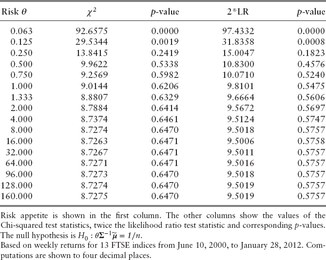
Table 9.7 shows likelihood ratio and Chi-squared tests for a multivariate tangency portfolio. For this purpose an equally weighted portfolio of the 11 FTSE indices is considered. The null hypothesis is that the equally weighted portfolio is a (multivariate) tangency portfolio with a specified risk appetite. That is

For the purpose of illustration, risk appetite takes values from 0.063 to 160. The columns of Table 9.7 show the values of the Chi-squared test statistics and twice the likelihood ratio test statistic. Not surprisingly, the values, and hence the computed p-values, are very similar. The implication is that, in practice, the Chi-squared test, which is simpler to compute, may be used. The table shows that for very small values of risk appetite, the null hypothesis that an equally weighted portfolio is a tangency portfolio is rejected. However, as risk appetite increases, it is impossible to reject the null hypothesis.

No empirical results are presented for the maximum Sharpe ratio portfolio. This is in keeping with the theoretical results described earlier, which is that maximum Sharpe ratio portfolio has infinite variance. In addition to being a volatile point on the efficient frontier, it is clear that tests of the type described in this chapter would often not lead to rejection of the null hypothesis. That is, many portfolios would not be statistically distinct from the maximum Sharpe ratio portfolio.

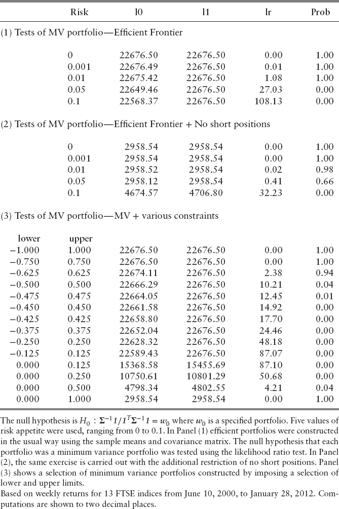
Tests of the minimum variance portfolio are reported in Table 9.8. For this, the null hypothesis is H₀ : Σ⁻¹ 1/1^T Σ⁻¹ 1 = w₀, where w₀ is specified portfolio. The results shown in Panel (1) of Table 9.8 were constructed as follows. Five values of risk appetite were used, ranging from 0 to 0.1. Efficient portfolios were constructed in the usual way, using the sample means and covariance matrix. The null hypothesis that each portfolio was a minimum variance portfolio was tested using the likelihood ratio test. As Panel (1) of Table 9.8 shows, at zero risk and risk equal to 0.001 and 0.01, the null hypothesis is not rejected. At higher levels of risk, it is rejected. In Panel (2) of Table 9.8, the same exercise is carried out with the additional restriction that no short positions are allowed. In this case, one can take a position higher up the frontier and still hold a portfolio that is not statistically distinguishable from the minimum variance portfolio. Panel (3) shows a number of minimum variance portfolios constructed by imposing a selection of lower and upper limits. As the panel shows, when the upper limit is unity, the null hypothesis is not rejected. There is a similar set of results that tests efficient frontier portfolios—that is, for the case where the null hypothesis is H₀ : Σ⁻¹1/1^TΣ⁻¹1 = w₀; Πμ = w₁. This table is omitted, but is available on request.

The final part of this empirical study is to examine the properties of the estimated risk appetite when an expected return target τ is set. Table 9.9 shows results for range of values of estimated expected excess return from −0.0014 to 0.0014. Table 9.9 shows the corresponding values of estimated risk appetite , its expected value, and volatility. These are computed using the estimated values of the standard constants. The expected value column indicates that is a biased estimator of θ. The volatility column shows that its effect is substantial for values of , which are small in magnitude. The remaining columns in Table 9.9 show lower and upper confidence limits at 99 percent, 95 percent, and 25 percent. These were computed using the integral representation of the distribution of . These three sets of limits show that the range of variability in is often large. For example, if the expected return target is set to , the overall estimated expected return on the portfolio is zero and the estimated risk appetite is equal to 0.0227. In this case, the chance that the true risk appetite is larger than 0.098 is 12.5 percent. There is also a 12.5 percent chance that it is less than −0.038. In short, the effect of estimation error on risk appetite may lead to a different position on the efficient frontier from that desired. The implications of this are discussed in the concluding section. It may also be noted that the distribution of is not normal and is skewed to the right (left) if θ is positive (negative).

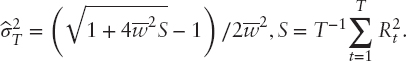
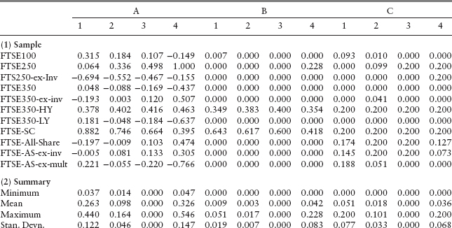
Variability in risk appetite will have an effect on estimated portfolio weights. This is illustrated in Table 9.10 for the case where the estimated expected return on the portfolio is zero. Table 9.10 has three vertical panels, headed A, B, and C. Panel A reports weights for efficient set portfolios—that is, portfolios constructed using only the budget constraint. Panel B includes the non–negativity constraint. Panel C seeks to achieve a degree of diversification by requiring that no weight exceed 0.2. In each of the three panels, there are four columns headed 1, 2, 3, and 4. These correspond to risk appetites −0.0381, 0.0227, 0, and 0.0981. These are, respectively, the lower 25 percent limit of , the estimated value, zero for the minimum variance portfolio, and the upper 25 percent limit. The horizontal panel numbered (1) shows the portfolio weights constructed using sample data. Panel (2) shows summary statistics for the absolute weight changes compared to the minimum variance portfolio. As panels (1) and (2) indicate, some weights are stable across the range of risk appetites, but many exhibit substantial variability. For comparison purposes, horizontal panels (3) and (4) show results when the sample covariance matrix is replaced with a shrinkage estimator. In this comparison, the shrinkage covariance matrix is

where denotes the average sample variance. Panels (3) and (4) show that the degree of instability in the portfolio weights is reduced, but that there are still significant changes for some assets.

DISCUSSION AND CONCLUDING REMARKS

This chapter is concerned with the vectors of estimated portfolio weights. It presents a synthesis of recent research and a summary of some new results. One objective of this article is to present a summary of the state of the art in a style and notation that is accessible. A second is to present some tests of efficiency that are straightforward to compute.

There is a closely related set of research that is concerned with the properties of the location, scale, and slope of the efficient frontier—that is, with the properties of the standard constants denoted collectively by α. Bodnar and Schmid (2008a) provide expressions for the probability distribution of the estimated return and estimated variance of an efficient frontier portfolio. They also provide expressions for moments up to order four. The corresponding distributions for the minimum variance portfolio are special cases. Essentially, the same results are given in the major paper by Kan and Smith (2008). The distributions typically involve nuisance parameters and are expressible as convolutions involving noncentral F distributions and the hyper geometric function ₁F₁. Nonetheless, there is a test for the curvature or slope of the efficient frontier that uses the noncentral F-distribution. There is a similar result for the slope of the efficient frontier when a risk-free asset is available. Building on their previous work, Bodnar and Schmid (2009) provide confidence sets for the efficient frontier.

Two notable results emerge from research in this area. First, when the effect of estimated parameters is taken into account, the maximum Sharpe ratio portfolio should probably be avoided in practice. This is because its moments are infinite. Second, using an estimated value of risk appetite, which is a consequence of setting an expected return target, leads to additional variability, both in portfolio weights and performance. It is difficult not to adhere to advice heard on more than one occasion: “Pick a point on the frontier that is suitable.” In other words, treat a suitable value of risk appetite as given.

The likelihood ratio tests described in this chapter are straightforward to compute. However, as they are asymptotic tests, they assume that the sample size is large. Construction of tests for small sample sizes may use exact distributions when these are available. These may be confounded by nuisance parameters. Furthermore, all results in this work and the majority of results reported in other papers make the standard IID normal assumptions. Bodnar and Schmid (2008a; 2008b) present results for elliptical distributions and for ARMA processes. Bodnar and Gupta (2011) study the effects of skewness on tests for the minimum variance portfolio, assuming that returns follow Azzalini multivariate skew-normal distributions. Overall, however, the tests reported here and elsewhere are appropriate for low-frequency applications based on large samples. For other types of portfolio selection, notably high-frequency applications, the tests may be computed but should probably be regarded only as rules of thumb for general guidance.

The third area of work mentioned in the introduction is that of the ex post performance of efficient portfolios. This has so far attracted relatively little attention. There are results in Kan and Smith (2008) and in Adcock (2013). Both sets of results indicate why ex post performance can be different from that expected ex ante, but also demonstrate the reliance of the results on standard assumptions about the distribution of asset returns.

Overall, many outstanding research challenges warrant further study.

REFERENCES

Adcock, C. J. 1997. Sample size determination: A review. Journal of the Royal Statistical Society. Series D (The Statistician) 46 (2): 261–283.

_________. 2013. Ex post efficient set mathematics. The Journal of Mathematical Finance 3 (1A): 201–210.

_________. 2014a. Mean-variance-skewness efficient surfaces, Stein's lemma and the multivariate extended skew-student distribution. The European Journal of Operational Research 234 (2): 392–401.

_________. 2014b. Likelihood Ratio Tests for Efficient Portfolios, Working Paper.

Adcock, C., N. Areal, M. R. Armada, M. C. Cortez, B. Oliveira, and F. Silva. 2012. Tests of the correlation between portfolio performance measures. Journal of Financial Transformation 35: 123–132.

Bawa, V., S. J. Brown, and R. Klein. 1979. Estimation Risk and Optimal Portfolio Choice, Studies in Bayesian Econometrics, Vol. 3. Amsterdam, North Holland.

Best, M. J., and R. R. Grauer. 1991. On the sensitivity of mean-variance-efficient portfolios to changes in asset means: Some analytical and computational results. Review of Financial Studies 4 (2): 315–342.

Britten-Jones, M. 1999. The sampling error in estimates of mean-variance efficient portfolio weights. Journal of Finance 54 (2): 655–672.

Bodnar, T., and A. K. Gupta. 2011. Robustness of the Inference Procedures for the Global Minimum Variance Portfolio Weights in a Skew Normal Model. The European Journal of Finance.

Bodnar, T., and Y. Okhrin. 2011. On the product of inverse wishart and normal distributions with applications to discriminant analysis and portfolio theory. Scandinavian Journal of Statistics 38 (2): 311–331.

Bodnar, T., and W. Schmid. 2008a. A test for the weights of the global minimum variance portfolio in an elliptical model. Metrika 67 (2): 127–143.

_________. 2008b. Estimation of optimal portfolio compositions for Gaussian returns. Statistics & Decisions 26 (3):179–201.

_________. 2009. Econometrical analysis of the sample efficient frontier. The European Journal of Finance 15 (3): 317–335.

Chopra, V., and W. T. Ziemba. 1993, Winter. The effect of errors in means, variances and covariances on optimal portfolio choice. Journal of Portfolio Management: 6–11.

Das Gupta, S. 1968. Some aspects of discrimination function coefficients. Sankhya A 30: 387–400.

Fang, K.-T., S. Kotz, and K.-W. Ng. 1990. Symmetric multivariate and related distributions. Monographs on Statistics and Applied Probability, Vol. 36. London: Chapman & Hall, Ltd.

Gibbons, M. R., S. A. Ross, and J. Shanken. 1989. A test of the efficiency of a given portfolio. Econometrica 57 (5): 1121–1152.

Huberman, G., and S. Kandel. 1987. Mean-variance spanning, The Journal of Finance, 42(4): 873–888.

Jobson, J. D., and B. Korkie. 1980. Estimation for Markowitz efficient portfolios, Journal of the American Statistical Association 75 (371): 544–554.

_________. 1989. A performance interpretation of multivariate tests of asset set intersection, spanning, and mean-variance efficiency. Journal of Financial and Quantitative Analysis 24 (2): 185–204.

Johnson, N., and S. Kotz. 1970. Continuous Univariate Distributions 2. Boston: John Wiley and Sons.

Kan, R., and D. R. Smith. 2008. The distribution of the sample minimum-variance frontier, Management Science 54 (7): 1364–1360.

Kandel, S. 1983. Essay no. I: A Likelihood Ratio Test of Mean Variance Efficiency in the Absence of a Riskless Asset, Essays in Portfolio Theory. Ph.D. dissertation (Yale University), New Haven, CT.

_________. 1984. The likelihood ratio test statistic of mean-variance efficiency without a riskless asset. Journal of Financial Economics 13 (X): 575–592.

Landsman, Z., and J. Nešlehová. 2008. Stein's Lemma for elliptical random vectors. Journal of Multivariate Analysis 99 (5): 912–927.

Liu, J. S. 1994. Siegel's Formula via Stein's Identities. Statistics and Probability Letters, 21(3): 247–251.

Markowitz, H. 1952. Portfolio selection. Journal of Finance 7 (1): 77–91.

Merton, R. 1972. An analytical derivation of the efficient portfolio frontier, Journal of Financial and Quantitative Analysis 7 (4): 1851–1872.

Muirhead, R. J. 1982. Aspects of Multivariate Statistical Theory. New York: John Wiley and Sons.

Okhrin, Y., and W. Schmid. 2006. Distributional properties of portfolio weights, Journal of Econometrics 134 (1): 235–256.

Ross, S. A. 1980. A test of the efficiency of a given portfolio, Paper prepared for the World Econometrics Meetings, Aix-en-Provence.

Scheffé, H. 1959. The Analysis of Variance. New York: John Wiley & Sons.

Sentana, E. 2009. The econometrics of mean-variance efficiency tests: A survey. The Econometrics Journal 12 (3): 65–101.

Siskind, V. 1972. Second moments of inverse Wishart-matrix elements. Biometrika 59 (3): 690.

Smith, T. M. F. 1976. The foundations of survey sampling: a review. Journal of the Royal Statistical Society, Series A 139 (2): 183–195.

Stein, C. M. 1981. Estimation of the mean of a multivariate normal distribution. Annals of Statistics 9 (6): 1135–1151.