
CHAPTER 8
Portfolio Optimization and Transaction Costs
University of Brescia,
Department of Information Engineering
Wlodzimierz Ogryczak
Warsaw University of Technology,
Institute of Control and Computation Engineering
M. Grazia Speranza
University of Brescia,
Department of Economics and Management
INTRODUCTION
In financial markets, expenses incurred when buying or selling securities are commonly defined as transaction costs and usually include brokers’ commissions and spreads (i.e., the difference between the price the dealer paid for a security and the price the buyer pays). Broadly speaking, the transaction costs are the payments that banks and brokers receive for performing transactions (buying or selling securities). In addition to brokerage fees/commissions, the transaction costs may represent capital gain taxes and thus be considered in portfolio rebalancing. Transaction costs are important to investors because they are one of the key determinants of their net returns. Transaction costs diminish returns and reduce the amount of capital available to future investments. Investors, in particular individual ones, are thus interested to the amount and structure of transaction costs and to how they will impact their portfolios.
The portfolio optimization problem we consider is based on a single-period model of investment, which is based on a single decision at the beginning of the investment horizon (buy and hold strategy). This model has played a crucial role in stock investment and has served as basis for the development of modern portfolio financial theory (Markowitz 1952 and 1959).
We consider the situation of an investor who allots her/his capital among various securities, assigning a share of the capital to each one. During the investment period, the portfolio generates a random rate of return. At the end of the period, the value of the capital will be increased or decreased with respect to the invested capital by the average portfolio return. Let N = {1, 2, …, n} denote a set of securities considered for an investment. For each security j ∈ N, the rate of return is represented by a random variable Rj with a given mean μj = ![]() {Rj}. Further, let x = (xj)j=1,…,n denote a vector of decision variables xj expressing the shares of capital in terms of amounts defining a portfolio. Each portfolio x defines a corresponding random variable
{Rj}. Further, let x = (xj)j=1,…,n denote a vector of decision variables xj expressing the shares of capital in terms of amounts defining a portfolio. Each portfolio x defines a corresponding random variable ![]() that represents the portfolio return. The mean return for portfolio x is given as
that represents the portfolio return. The mean return for portfolio x is given as ![]() . To represent a portfolio, the shares must satisfy a set P of constraints that form a feasible set of linear inequalities. This basic set of constraints is defined by the requirement that the amount invested (shares of the capital) must sum to the capital invested C, and that short selling is not allowed:
. To represent a portfolio, the shares must satisfy a set P of constraints that form a feasible set of linear inequalities. This basic set of constraints is defined by the requirement that the amount invested (shares of the capital) must sum to the capital invested C, and that short selling is not allowed:

We use the notation C to denote the capital available, when it is a constant. Later we will use the notation C to denote the capital investment, when it is a problem variable.
An investor usually needs to consider some other requirements expressed as a set of additional side constraints (e.g. thresholds on the investment). Most of them can be expressed as linear equations and inequalities (see Mansini et al. 2014).
Following the seminal work by Markowitz (1952), we model the portfolio optimization problem as a mean-risk bicriteria optimization problem
where the mean μ(x) is maximized and the risk measure ![]() (x) is minimized. We will say that a risk measure is LP computable if the portfolio optimization model takes a linear form in the case of discretized returns (see Mansini et al. 2003a). We will consider as risk measure the mean semi-absolute deviation (semi-MAD) that is an LP computable risk measure.
(x) is minimized. We will say that a risk measure is LP computable if the portfolio optimization model takes a linear form in the case of discretized returns (see Mansini et al. 2003a). We will consider as risk measure the mean semi-absolute deviation (semi-MAD) that is an LP computable risk measure.
One of the most basic results in traditional portfolio optimization theory is that small investors choose well-diversified portfolios to minimize risk. However, in contrast to theory, noninstitutional investors usually hold relatively undiversified portfolios. While there may be specific motivations for this behavior, it is recognized both in the literature and by practitioners that this is also due to the presence of transaction costs and, in particular, of fixed transaction costs. The introduction of fixed transaction costs may require the use of binary variables. It is known that finding a feasible solution to a portfolio optimization problem with fixed costs is an NP-complete problem (see Kellerer et al. 2000). This implies that, even with an LP computable risk function, a portfolio optimization problem which includes transaction costs may turn out to be a complex problem to solve.
The objective of this work is the analysis of the impact of transaction costs on portfolio optimization. We overview the most commonly used transaction cost structures and discuss how the transaction costs are modeled and embedded in a portfolio optimization model.
This chapter is organized as follows. In the second section the literature on portfolio optimization with transaction costs is surveyed. The focus is on transaction costs incurred by small investors with a buy and hold strategy, but we also briefly analyze contributions on transaction costs in portfolio rebalancing. Essentially, with respect to the single-period problem, in the portfolio rebalancing problem, the investor makes investment decisions starting with a portfolio rather than cash, and consequently some assets must be liquidated to permit investment in others. In the third section, we introduce some portfolio optimization models based on LP computable risk measures. In the fourth section, we discuss the main structures of transaction costs, their mathematical formulations, and how they can be incorporated in a portfolio optimization model. Following the most traditional financial literature on portfolio optimization, we classify transaction costs as fixed and variable. While convex piecewise linear cost functions can be dealt with using linear constraints in a continuous setting, concave piecewise linear cost functions require the introduction of binary variables to be modeled using linear constraints. In the fifth section, we provide an example that shows how the portfolio optimization with transaction costs may lead to a discontinuous efficient frontier and therefore to a nonunique solution when minimizing the risk under a required expected return (a similar result for portfolio optimization with cardinality constraint can be found in Chang et al. 2000). This result motivates the introduction of a regularization term in the objective function in order to guarantee the selection of an efficient portfolio. This modified model has been used in the computational testing. Finally, the last section is devoted to the experimental analysis. We provide a comparison of three simplified cost structures on a small set of securities taken from a benchmark data set. The experiments show that the impact of the transaction costs is significant, confirming the findings of the recent work by Chen et al. (2010) on the mean–variance framework and those of the well-known work by Chen et al. (1971) showing that lower revision frequency may reduce the magnitude of transaction costs in a rebalancing context.
LITERATURE REVIEW ON TRANSACTION COSTS
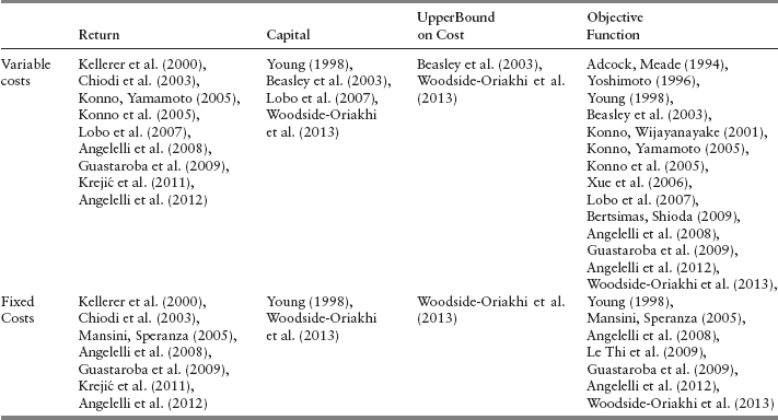
The impact of the introduction of real features in a portfolio optimization model has been largely discussed in the literature (see the recent survey by Mansini et al. 2014). The focus of this section will be on transaction costs that are among the most relevant real features. In financial markets, transaction costs are entailed by purchases and sales of securities and are paid both in case of portfolio revision and in case of buy and hold investments. Contributions from the literature are analyzed in chronological order, specifying if referring to a single-period portfolio optimization problem or to a rebalancing problem. Moreover, for each analyzed reference we specify which type of cost (fixed and/or variable) is considered and how costs are embedded into a portfolio optimization model. We summarize the contributions in Table 8.1, where the references are classified according to the way in which the transaction costs are modeled. As we will see later in more detail, the transaction costs may be deducted from the return (second column of Table 8.1), reduce the capital available for the investment (third column), be bounded (fourth column), or be considered in the objective function, typically the risk function (last column).
It is well known that excluding transaction costs may generate inefficient portfolios (see Arnott and Wagner 1990). An interesting question is whether the performance of a buy and hold strategy may be improved by a periodic revision of the portfolio (see Chen et al. 2010). A first study in this direction is a model due to Chen et al. (1971), which is a portfolio revision model where transaction costs are included in Markowitz model as a constant proportion of the transacted amount. The costs, incurred to change the old portfolio to the new one, are deduced from the ending value of the old portfolio. Afterward, Johnson and Shannon (1974) showed experimentally that a quarterly portfolio revision may outperform a buy and hold policy. Their findings, however, do not consider transaction costs.
While variable transaction costs make individual securities less attractive, fixed transaction costs are usually a reason for holding undiversified portfolios. The first detailed analysis on portfolio selection with fixed costs can be attributed to Brennan (1975). The author introduced a model for determining the optimal number of securities in the portfolio. Earlier, Mao (1970), Jacob (1974), and Levy (1978) considered the fixed transaction cost problem, avoiding, however, a direct modeling but placing instead restrictions on the number of securities. Afterward, Patel and Subrahmanyam (1982) criticized Brennan's approach as based on the capital asset pricing theory when it is well known that this pricing relationship is affected if trading costs are taken into account (see Levy (1978) for a theoretical proof). They introduced transaction costs by placing restrictions on the variance-covariance matrix.
Adcock and Meade (1994) considered the problem of rebalancing a tracking portfolio over time, where transaction costs are incurred at each rebalancing. They introduced the costs in the objective function by adding a linear term to the risk term of the mean-variance model. Yoshimoto (1996) introduced instead a V-shaped function representing a proportional cost applied to the absolute difference between an existing and a new portfolio. The proposed model considered the transaction costs in the portfolio return that was optimized in a mean-variance approach. The author examined the effect of transaction costs on portfolio performance.
Young (1998) extended his linear minimax model to include for each security both a fixed cost and a variable cost for unit purchased. This is one of the first papers directly accounting for fixed transaction costs. The author underlined the importance of the investment horizon when computing the net expected return. In particular, he made an explicit assumption on the number of periods P in which the portfolio would be held. The net expected return was then computed by multiplying the portfolio return by P and then subtracting the transaction costs. The solved problem maximized the net return and considered the costs also in the capital constraint.
Mansini and Speranza (1999) dealt with a portfolio optimization problem with minimum transaction lots where the risk was measured by means of the mean semi-absolute deviation. They also considered proportional transaction costs modifying directly the securities price. Also, Crama and Schyns (2003) did not incorporate transaction costs in the objective function or in the constraints, but imposed upper bounds on the variation of the holdings from one period to the next in a mean-variance model.
In Kellerer et al. (2000) the authors studied a problem with fixed and proportional costs, and possibly with minimum transaction lots. They formulated different mixed-integer linear programming models for portfolio optimization using the mean semi-absolute deviation as risk measure. The first model considered the case in which the investor pays for each selected security a fixed sum plus a proportional cost as a percentage of the amount invested. The second model dealt with the case where along with proportional costs a fixed cost for each security is taken into account that is charged only if the sum of money invested in the individual security exceeds a predefined bound. In the models, the costs were introduced only in the return constraint. In computational experiments, the authors showed that fixed costs influence portfolio diversification and that the introduction of costs, much more than their amount, had a relevant impact on portfolio diversification. Such an impact was strengthened by the introduction of minimum lots.
Konno and Wijayanayake (2001) analyzed a portfolio construction/rebalancing problem under concave transaction costs and minimal transaction unit constraints. The concave transaction cost for each security was assumed to be a nonlinear function of the investment (a nondecreasing concave function up to certain invested amount). This modeled the situation where the unit transaction cost is relatively large when the amount invested is small, and gradually decreases as amount increases. In fact, the unit transaction cost may increase beyond some point, due to illiquidity effects, and become convex. The authors, however, assumed that the amount of investment (disinvestment) is below that point and that the transaction cost was defined by a well specified concave function. They adopted the absolute deviation of the rate of return of the portfolio as risk measure. The net return, after payment of the transaction costs, was maximized while the risk was bounded in the constraints. A branch and bound algorithm was proposed to compute an optimal solution.
Chiodi et al. (2003) considered mutual funds as assets on which to build a portfolio. They proposed a mixed-integer linear programming model for a buy-and-hold strategy, with the mean semi-absolute deviation as risk measure where variable (commissions to enter/leave the funds) and fixed (management fees) costs were included. In particular, they analyzed a classical type of entering commissions where the applied commission rate decreases when the capital invested increases and assuming as null the leaving commission, which is the case of an investor who does not leave the fund as long as leaving commissions are charged. The entering cost function was a concave piecewise linear function, and binary variables were introduced to correctly model the problem. The costs were considered only in the expected return constraint.
Beasley et al. (2003) analyzed the index tracking problem (i.e., the problem of reproducing the performance of a stock market index without purchasing all of the stocks that make up the index), and explicitly included transaction costs for buying or selling stocks. They suggested a new way of dealing with transaction costs by directly imposing a limit on the total transaction costs that could be incurred. This was a way to prevent the costs to become excessive. Costs were then introduced in the capital constraint to reduce the amount of cash available for the reinvestment. As stated by the authors, the majority of the work on index tracking presented in the literature does not consider transaction costs.
In Mansini and Speranza (2005) the authors considered a single-period mean-safety portfolio optimization problem using the mean downside underachievement as performance measure (i.e., the safety measure corresponding to the mean semi-absolute deviation). The problem considered integer constraints on the amounts invested in the securities (rounds) and fixed transaction costs enclosed in both the constraint on the expected return and the objective function. The paper presented one of the first exact approaches to the solution of a portfolio optimization model with real features.
In Konno and Yamamoto (2005) the authors analyzed a portfolio optimization problem under concave and piecewise constant transaction cost. They formulated the problem as non-concave maximization problem under linear constraints using the absolute deviation as a measure of risk. Konno et al. (2005) proposed a branch and bound algorithm for solving a class of long-short portfolio optimization problems with concave and d.c. (difference of two convex functions) transaction cost and complementary conditions on the variables. They maximized the return subject to a bound on the absolute deviation value of the portfolio.
Xue et al. (2006) studied the classical mean-variance model modified to include a nondecreasing concave function to approximate the original transaction cost function, as described by Konno and Wijayanayake (2001). In the resulting model, costs were treated only in the objective function. A branch-and-bound algorithm was proposed to solve the problem.
Best and Hlouskova (2005) considered the problem of maximizing an expected utility function of a given number of assets, such as the mean-variance or power-utility function. Associated with a change in an asset holding from its current or target value, the authors considered a transaction cost. They accounted for the transaction costs implicitly rather than explicitly.
Lobo et al. (2007) dealt with a single-period portfolio optimization by assuming a reoptimization of a current portfolio. They considered the maximization of expected return, taking transaction costs into account in the capital constraints or as an alternative, minimizing the transaction costs subject to a minimum expected return requirement.
Angelelli et al. (2008) considered two different mixed-integer linear programming models for solving the single-period portfolio optimization problem, taking into account integer stock units, transaction costs, and a cardinality constraint. The first model was formulated using the maximization of the worst conditional expectation. The second model was based on the maximization of the safety measure associated with the mean absolute deviation. In both models, proportional and fixed costs had to be paid if any positive amount was invested in a security. Costs were deducted from the expected return and the net returns were also considered in the objective function.
In Bertsimas and Shioda (2009) the authors focused on the traditional mean-variance portfolio optimization model with cardinality constraint. They also considered some costs reflecting the stock price impact derived from purchase or sale orders. The magnitude of the costs depended on the particular stock and on the trade sizes: large purchase orders increased the price whereas large sale orders decreased the price of the stock. Assuming symmetric impact for purchases and sales, the authors modeled this effect by a quadratic function included only in the objective function.
Le Thi et al. (2009) addressed the portfolio optimization under step-increasing transaction costs. The step-increasing functions were approximated, as closely as desired, by a difference of polyhedral convex functions. They maximized the net expected return.
Guastaroba et al. (2009) modified the single-period portfolio optimization model to introduce portfolio rebalancing. They used the conditional value at risk (CVaR) as measure of risk and studied the optimal portfolio selection problem considering fixed and proportional transaction costs in both the return constraint and the objective function.
Baule (2010) studied a direct application of classical portfolio selection theory for the small investor, taking into account transaction costs in the form of bank and broker fees. In particular, the problem maximized the single-period expected utility and introduced cost in the form of proportional cost with minimum charge, that is cost was constant up to a defined amount. Above this amount, cost was assumed to increase linearly. The analysis was made in terms of tangent portfolio.
Krejić et al. (2011) considered the problem of portfolio optimization under value at risk (VaR) risk measure, taking into account transaction costs. Fixed costs as well as impact costs as a nonlinear function of trading activity were incorporated in the optimal portfolio model that resulted to be a nonlinear optimization problem with nonsmooth objective function. The model was solved by an iterative method based on a smoothing VaR technique. The authors proved the convergence of the considered iterative procedure and demonstrated the nontrivial influence of transaction costs on the optimal portfolio weights. More recently, Woodside-Oriakhi et al. (2013) considered the problem of rebalancing an existing portfolio, where transaction costs had to be paid if the amount held of any asset was varied. The transaction costs may be fixed and/or variable. The problem was modeled as a mixed-integer quadratic program with an explicit constraint on the amount to pay as transaction costs.
Angelelli et al. (2012) proposed a new heuristic framework, called Kernel Search, to solve the complex problem of portfolio selection with real features such as cardinality constraint. They considered fixed and proportional transaction costs inserted in both return constraint and objective function represented by CVaR maximization.
AN LP COMPUTABLE RISK MEASURE: THE SEMI-MAD
While the classical risk measure, from the original Markowitz model (1952), is the standard deviation or variance, several other performance measures have been later considered, giving rise to an entire family of portfolio optimization models (see Mansini et al. 2003b and 2014). It is beyond the scope of this chapter to discuss the different measures. In order to have a complete modeling framework and also in view of the computational testing, we choose one of the most popular LP computable risk measures, the semi-mean absolute deviation (semi-MAD). To make this chapter self-contained, we briefly recall the basic portfolio optimization model with the semi-MAD as risk function.
We consider T scenarios with probabilities pt, t = 1, …, T, and assume that for each random variable Rj its realization rjt under the scenario t is known and ![]() . Typically, the realizations are derived from historical data. Similar to the mean μ(x), the realizations of the portfolio returns Rx are given by
. Typically, the realizations are derived from historical data. Similar to the mean μ(x), the realizations of the portfolio returns Rx are given by ![]() .
.
The mean absolute deviation (MAD) model was first introduced by Konno and Yamazaki (1991) with the mean absolute deviation δ(x) as risk measure. The MAD is the mean of the differences between the average portfolio return (or rate of return in case the investments are expressed in shares and not in amounts) and the portfolio return in the scenarios, where the differences are taken in absolute value. The semi-MAD was introduced in Speranza (1993) as the mean absolute downside deviation, where the mean is taken only over the scenarios where the return is below the average portfolio return. The mean absolute downside deviation is equal to the mean upside deviation and equal to half the MAD. The measure is simply referred to as semi-MAD and indicated as δ(x), with
![]()
Adopting the semi-MAD as risk measure gives rise to portfolio optimization models that are equivalent to those adopting the MAD. For discrete random variables, the semi-MAD is LP computable as follows (see Mansini et al. 2003b for details):
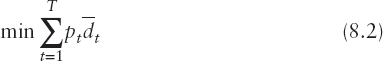
where variable dt, t = 1, …, T, represents the portfolio semi-deviation under scenario t that is, the difference between the average portfolio return and the portfolio return under scenario t. We refer to this model as the basic semi-MAD model.
In order to guarantee the mean-risk efficiency of the optimal solution even in the case of discontinuous efficient frontier, we consider the regularized MAD model:

thus differing from the basic semi-MAD model (8.2) to (8.7) only due to the objective function combining the original risk measure with the expected return discounted by an arbitrary small positive number ε.
Note that the SSD consistent (Ogryczak and Ruszczyński 1999) and coherent MAD model with complementary safety measure, μδ(x) = μ(x) − δ(x) = ![]() { min { μ(x), Rx } } (Mansini et al. 2003a), leads to the following LP minimization problem:
{ min { μ(x), Rx } } (Mansini et al. 2003a), leads to the following LP minimization problem:

which is a special case of (8.8).
MODELING TRANSACTION COSTS
We define available capital as the total amount of money that is available to an investor, both for the investment in securities and possible additional costs. In general, part of this money may be left uninvested. The invested capital is the capital strictly used for the investment and that yields a return.
Frequently, in portfolio optimization models the invested capital coincides with the available capital and is a constant, which is the case in the basic semi-MAD model (8.2)–(8.7). Being a constant, capital C can be normalized to 1, while the amount invested in each security can be expressed as share by the linear transformation wj = xj/C. Although in many cases the modeling of the investment in a security as amount or share is irrelevant, there are cases, as when transaction lots are considered, where the use of amounts instead of shares, is necessary (see Mansini and Speranza 1999). This is the reason why from the beginning of this paper we have used the value C of the available capital, and the amounts xj as variables in the portfolio optimization.
When considering transaction costs in portfolio optimization models, two main modeling issues have to be analyzed:
- the structure of the transaction costs;
- how the transaction costs are incorporated into a portfolio optimization model.
In the following, we will develop these two issues. For the sake of simplicity, we will restrict the presentation to a buy-and-hold strategy of the kind considered in the Markowitz model, where a portfolio is constructed and not rebalanced.
Structure of the Transaction Costs
Transaction costs are commonly classified as fixed and variable. For each of these two classes, we will analyze the most common cost functions. General cost functions may not be linear; see, for instance, the concave cost function dealt with in Konno and Wijayanayake (2001). With concave transaction costs, the portfolio optimization problem becomes nonlinear and hard to solve, even without binary or integer variables. For this reason, concave functions are often approximated by piecewise linear functions.
Let us indicate with K(x) the transaction cost function for portfolio x. We will assume that transaction costs are charged on each security, independently of the investment in the others. Thus, we restrict our analysis to functions that are separable, such that
Fixed Costs A fixed transaction cost is a cost that is paid for handling a security independently of the amount of money invested. The total transaction cost for security j can be expressed as:

where fj is the transaction cost paid if security j is included in the portfolio.
To include fixed costs in a mathematical programming model we need binary variables zj, one for each security j, j ∈ N. Variable zj must be equal to 1 when security j is selected in the portfolio, and to 0 otherwise. Constraints need to be added that impose that zj is equal to 1 if xj > 0 and 0 otherwise. Typical linear constraints are
where lj, uj are positive lower and upper bounds on the amount invested on security j, with uj possibly equal to C. These constraints impose that if xj > 0 then zj = 1, and that if xj = 0 then zj = 0.
From now on, we identify the above cost structure imposing a fixed cost fj for each selected security j as pure fixed cost (PFC) (see Figure 8.1, left-hand side). This is one of the most common cost structures applied by financial institutions to investors.
Variable Costs Variable transaction costs depend on the capital invested in the securities and may have different structures. We divide variable transaction cost functions into linear (proportional) cost functions, convex and concave piecewise linear cost functions. In all cases the transactions costs Kj(x) are introduced through variables kj(j ∈ N) defined by appropriate relations to other model variables.
Linear Cost Function Proportional transaction costs are the most used in practice and the most frequently analyzed in the literature. In this case, a rate cj is specified for each security j ∈ N as a percentage of the invested amount in the security:
and ![]() . We call this cost structure pure proportional cost (PPC).
. We call this cost structure pure proportional cost (PPC).

FIGURE 8.1 Pure fixed cost structure (left-hand figure) and proportional cost with minimum charge structure (right-hand figure).
Convex Piecewise Linear Cost Function We consider here the case where each Kj(xj), j ∈ N, is a convex piecewise linear function. Convex piecewise linear costs are not frequently used in practice, but can be encountered as leaving commissions for mutual funds and model some cost components as taxes. A different rate cji is applied to each, nonoverlapping with others, interval i ∈ I of capital invested in security j, j ∈ N, that is:

where M1,…, M|I|−1 are the extremes defining the intervals into which the capital is divided. Note that, without loss of generality, we can always assume that also the last interval (M|I|−1, ∞) has a finite upper bound M|I| corresponding to the maximum amount that can be invested in a security, that is, the whole capital C.
As Kj(xj) is convex, the rates cji are increasing, that is, cj1 < cj2 < cj3 < … < cj|I|. In Figure 8.2, we show an example of a three intervals convex piecewise linear function.

This case is easy to model in terms of linear constraints and continuous variables when the costs are minimized within the optimization model (Williams 2013). Namely, introducing one continuous variable xji for each interval i ∈ I, the investment xj in security j can be expressed as the sum of all auxiliary variables xji as:
and the transaction cost function as:
with the additional constraints:
This LP model guarantees only inequalities kj ≥ Kj(xj), which is enough when relying on optimization model to enforce minimal costs if possible. In fact, due to the increasing cost rates, a sensible complete optimization model should be such that it is not beneficial to activate variable xji unless all variables with a smaller cost rate are saturated. Unfortunately, as demonstrated further, it is not always the case in portfolio optimization where a risk measure is minimized.
Therefore, to represent equations not relying on optimization process, we should also include constraints that impose that, if variable xji takes a positive value, all variables xjk, k = 1, …, i − 1, are set to their upper bounds. For this purpose, one needs to implement implications by binary variables replacing (8.15)–(8.19) with the following:

where yj2, …, yj,|I| are binary variables.
Concave Piecewise Linear Cost Function Each cost function Kj(xj), j ∈ N is here a piecewise linear concave function. In this case, the rates cji are decreasing, that is, cj1 > cj2 > cj3 > … > cj|I|. This structure of transaction costs is commonly applied by financial institutions and frequently appears as entering commission for mutual funds. These costs are also studied in the literature for the market illiquidity effect described in Konno and Wijayanayake (2001). In Figure 8.3, we show an example of a four intervals concave piecewise linear function, where M4 = C.
Contrary to the case of convex functions, in a “sensible” complete model, the variable xji has a smaller rate and thus is more convenient than all variables xjk, k = 1, …, i − 1 associated with the preceding intervals. Then, we always need here additional binary variables, one for each interval, as in (8.20) – (8.23).
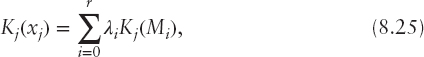
Another model can be built when having available the list of all breaking points for the cost function. In addition to the r breaking points (M1, Kj(M1)), …, (Mr, Kj(Mr)), we have the starting point (M0, Kj(M0)) corresponding to the origin (0, 0). Again, we can assume that the last breaking point is Mr = C. For example, in Figure 8.3 we have four breaking points, plus the origin. We know that each line segment can be expressed as the convex combination of its extremes. Then, if Mi ≤ x ≤ Mi+1, x can be expressed as x = λiMi + λi+1Mi+1 with λi + λi+1 = 1, λi, λi+1 ≥ 0, we correctly obtain Kj(x) = λiKj(Mi) + λi+1Kj(Mi+1) (see, for instance, the line segment between (M1, Kj(M1)) and (M2, Kj(M2)) in Figure 8.3). Thus, we have to consider each single line segment connecting two consecutive breaking points and use additional binary variables yi, i = 0, …, r − 1, where yi = 1 if Mi ≤ x ≤ Mi+1 and yi = 0 otherwise. The resulting linear constraints are (see Williams 2013):


and
with constraints on variables as follows:
Note that, thanks to these constraints, only pairs of adjacent coefficients λi are allowed to be strictly positive.
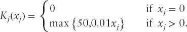
Linear Function with Minimum Charge In practice, a common piecewise linear cost function frequently used by financial institutions has the structure shown in Figure 8.1 (right-hand side). This structure models a situation where a fixed cost fj is charged for any invested amount lower than or equal to a given threshold M = fj/cj and then, for an investment greater than M, a proportional cost cj is charged:

We call this cost structure proportional cost with minimum charge (PCMC). This cost structure is convex piecewise linear with a discontinuity at xj = 0. The inequality kj ≥ Kj(xj) with, thus, the model relying on optimization of transaction costs can be easily built with inequalities:
where yj are binary variables.
In order to get a model not relying on the optimization (and thus imposing equality kj = Kj(xj)), one needs to build the corresponding model (8.20)–(8.23), together with a defined minimal investment level lj and corresponding fixed charge inequalities:
with the cost formula:
where yj1 and yj2 are binary variables.
Transaction Costs in Portfolio Optimization
Now, we will discuss the most common ways to embed transaction costs in a complete portfolio optimization model:
- Costs in the return constraint: Transaction costs are considered as a sum (or a percentage, in case of shares instead of amounts) directly deducted from the average portfolio return (rate of return, in case of shares instead of amounts). This assumption is reasonable in a single-period investment, provided that the investor has a clear idea of the length of his/her investment period when deducting such an amount from the return. We will clarify this concept later.
- Costs in the capital constraint: Transaction costs reduce the capital available. In this case, the invested capital is different from the initial capital and is not a constant but depends on the transaction costs paid, that is, on the portfolio. This way of dealing with transaction costs is more frequent in rebalancing problems.
In addition to the two main ways of considering transaction costs, one may also impose an upper bound on the total transaction costs paid (see, e.g., Beasley et al. 2003).
Let us now consider each of the two aforementioned main cases separately.
Costs in the Return Constraint In this case, the classical constraint on the expected return on the portfolio is modified as follows:
This models the situation where the transaction costs are charged at the end of the investment period.
As mentioned earlier, the introduction of the transaction costs in the return constraint correctly models the problem if the investor has an investment horizon in mind (see also Young 1998). To clarify the concept, we consider an example. Let us assume that a proportional cost equal to 0.20 percent for each transaction is charged. If the investment horizon is one year, a percentage 0.20 percent will have to be deducted from each return rate μj, computed on a yearly basis, in constraint (8.36). If, on the contrary, the horizon is of one month only, then the percentage 0.20 percent will have to be deducted from the return rate μj computed this time on a monthly basis. In the last case, the impact of the transaction costs is much higher. Obviously, the portfolios generated will be different.
This approach essentially depends on the assumption that the transaction costs only decrease the final return. This means we are focused on the net return ![]() . Hence, in comparison to the original distribution of returns, the net returns are represented with a distribution shifted by the transaction costs. Such a shift directly affects the expected value
. Hence, in comparison to the original distribution of returns, the net returns are represented with a distribution shifted by the transaction costs. Such a shift directly affects the expected value ![]() . On the other hand, for shift-independent risk measures like the MAD, we get for the net returns the same value of risk measure as for the original returns
. On the other hand, for shift-independent risk measures like the MAD, we get for the net returns the same value of risk measure as for the original returns ![]() . This means such a risk measure minimization is neutral with respect to the transaction costs, and it does not support the cost minimization. When using this risk minimization, one needs to use exact models for transactions cost calculation, models that do not rely on optimization to charge the correct amount of the transaction costs. In addition, one may face another difficulty related to discontinuous efficient frontier and non-unique optimal solution (possibly inefficient). All these problems can be solved, if the risk minimization is regularized with the introduction of an additional term on mean net return. Actually, there is no such problem when coherent (safety) forms of risk measures are used. Optimization based on such measures supports costs minimization and therefore allows us for simpler cost models while guaranteeing efficient solutions.
. This means such a risk measure minimization is neutral with respect to the transaction costs, and it does not support the cost minimization. When using this risk minimization, one needs to use exact models for transactions cost calculation, models that do not rely on optimization to charge the correct amount of the transaction costs. In addition, one may face another difficulty related to discontinuous efficient frontier and non-unique optimal solution (possibly inefficient). All these problems can be solved, if the risk minimization is regularized with the introduction of an additional term on mean net return. Actually, there is no such problem when coherent (safety) forms of risk measures are used. Optimization based on such measures supports costs minimization and therefore allows us for simpler cost models while guaranteeing efficient solutions.
Costs in the Capital Constraint If the transaction costs are accounted for in the capital constraint, the invested capital becomes a variable C, in general different from the initial available capital C. The invested capital will be

when the initial capital is entirely used, either in investment or in transaction costs, which is the most common case and the natural extension of the classical Markowitz model. In this case, when using amounts (with respect to shares), risk decreases due to decreased invested capital. This means that higher transaction costs result in lower absolute risk measure value (Woodside-Oriakhi et al. 2013). Such an absolute risk minimization may be simply achieved due to increasing transaction costs. Transaction costs must be then modeled exactly (with equality relations). This applies also to the coherent (safety) measures. To get better results, one should use rather relative risk measurement dividing by the invested capital. However, the invested capital is a variable thus leading to the ratio criteria, which creates further complications. For instance, in Mitchell and Braun (2013) the authors considered convex transaction costs incurred when rebalancing an investment portfolio in a mean-variance framework. In order to properly represent the variance of the resulting portfolio, they suggested rescaling by the funds available after paying the transaction costs.
In our computational analysis, we have focused on the costs in the return constraint approach as more popular and better suited for risk-minimization models with amounts as decision variables, rather than shares.
NON-UNIQUE MINIMUM RISK PORTFOLIO
The problem of non-unique minimum risk portfolios with bounded (required) expected return may arise also when transaction costs are ignored. As a very naive example, one may consider a case where two risk-free assets are available with different returns but both meeting the required expected return.
In the following we show a nontrivial example of non-unique solution for the case of proportional transaction costs with minimum charge.
Example
Let us consider the case of proportional transaction costs with minimum charge (see Figure 8.1, right-hand side). Let us assume fj = 50 while the proportional cost is on the level of 1 percent; that is, cj = 0.01.
Consider a simplified portfolio optimization problem having three assets available with rates of return represented by r.v. R1, R2, and R3, respectively. They are defined by realizations rjt under three equally probable scenarios St, t = 1, 2, 3, as presented in Table 8.2. Thus, the expected rates of return are given as 0.1567, 0.1507, and 0.1492, respectively. The capital to be invested is C = 10, 000.
Consider a portfolio (x1, x2, x3) defined by the shares of capital in terms of amounts defining a portfolio, x1 + x2 + x3 = C, thus generating rate of return represented by r.v. Rx = x1R1 + x2R2 + x3R3. The expected net return of the portfolio taking into account the transaction costs is given by the following formula:

Assume we are looking for minimum risk portfolio meeting the specified lower bound on the expected net return, say 14 percent—that is,
We focus our analysis on the risk measured with the mean absolute deviation. Note that our absolute risk measure is defined on distributions of returns not reduced by the transaction costs. However, the transaction costs are deterministic; this causes the same risk measure to remain valid for the net returns.
Finally, our problem of minimizing risk under the required return takes the following form:
One can find out that the required return bound may be satisfied by two single asset portfolios (C, 0, 0) and (0, C, 0), as well as by some two-asset portfolios with large enough share of the first asset, that is, portfolios (x1, x2, 0) built on R1 and R2 with x1 ≥ 43/160C, and portfolios (x1, 0, x3) built on R1 and R3with x1 ≥ 58/175C. On the other hand, no two-asset portfolio built on R2 and R3 and no three-asset portfolio fulfills the required return bound.
While minimizing the MAD measure, one can see that δ(C, 0, 0) = 0.04C/3 and δ(0, C, 0) = 0.02C/3. Among portfolios (x1, x2, 0) built on R1 and R2, the minimum MAD measure is achieved for δ(C/3, 2C/3, 0) = 0.02C/9. Similarly, among portfolios (x1, 0, x3) built on R1 and R3, the minimum MAD measure is achieved for δ(C/3, 0, 2C/3) = 0.02C/9. Thus, finally, while minimizing the MAD measure, one has two alternative optimal portfolios (C/3, 2C/3, 0) and (C/3, 0, 2C/3). Both portfolios have the same MAD value, but they are quite different with respect to the expected return. Expected return of portfolio (C/3, 0, 2C/3) is smaller than that of portfolio (C/3, 2C/3, 0). Therefore, portfolio (C/3, 0, 2C/3) is clearly dominated (inefficient) in terms of mean-risk analysis. While solving problem (8.39), one may receive any of the two min risk portfolios. It may be just the dominated one. Therefore, a regularized risk minimization must be used to guarantee selection of an efficient portfolio:
Note that such a regularization is not necessary if the corresponding safety measure is maximized instead of the risk measure minimization.
Details on the supporting calculations for the example presented in this section can be found in the Appendix.
EXPERIMENTAL ANALYSIS
In this section, we revisit the portfolio optimization problem with transaction costs, exploring the impact of transaction costs incurred in portfolio optimization using real data. We consider a capital invested equal to 100,000 euros, a unique set of 20 securities from Italian Stock Exchange with weekly rates of returns over a period of two years (T = 104), and three different values for the required rate of return, μ0 = 0, 5, 10 percent (on a yearly basis), respectively. The data set is available on the website of the book. We test and compare the three cost structures identified as pure fixed cost (PFC), pure proportional cost (PPC), and proportional cost with minimum charge (PCMC). As objective function, we consider the semi-MAD as risk measure (see (8.2)), the regularized semi-MAD (see (8.8)) and the semi-MAD as safety measure (see (8.9)), respectively. This means we solved 3 × 3 × 3 = 27 portfolio optimization instances altogether. Models were implemented in C++ using Concert Technology with CPLEX10.
In the Italian market, a small investor who wants to allocate her/his capital buying online a portfolio usually incurs in costs as shown in Table 8.3 (source is online information brochure provided by banks). These costs are applied by banks for reception and transmission of orders on behalf of the customers through online trading. Assets are from the Italian Stock Exchange. Dealing with foreign assets implies larger costs. Not all banks apply pure fixed costs. However, when available, the option implies a cost that varies from a minimum of 9 euros for transaction to a maximum of 12.
In the following experimental results, we assume that the proportional cost is equal to cj = 0.25 percent for all the securities in both the PPC and the PCMC cases. This value corresponds to the average percentage imposed by the banks. In particular, in PCMC the value M corresponding to the capital threshold under which a fixed charge is applied is set to 4,000 euros. This implies fj = 10 for all the securities. Finally, in case of a PFC structure, we assume fj = 10 euros for all the assets. Again, the value corresponds to the average value applied in practice.

In Table 8.4, we provide the results obtained when applying the PPC structure. The table is divided in three parts, one for each objective function, namely the semi-MAD (in the risk form), semi-MAD regularized with the introduction of an adjustment coefficient (ε = 0.05) (8.8), and the semi-MAD formulated as a coherent (safety) measure (8.9). For the first two parts the three columns correspond to three different required rates of return (on a yearly basis) set to 0 percent, 5 percent, and 10 percent, respectively. For the safety measure, we only provide the MSP (maximum safety portfolio) since for any μ0 lower than the expected net return of the MSP, the MSP is the optimal solution to the problem. Table 8.4 consists of six lines. Line “#” indicates the number of selected securities, while lines “min” and “max” provide the minimum (positive) and the maximum amounts per security invested in the portfolio; line “cost” shows the total cost paid in the transaction costs whereas line “net return” provides the portfolio return net of the transaction costs. Finally, “obj” reports the value of the objective function.
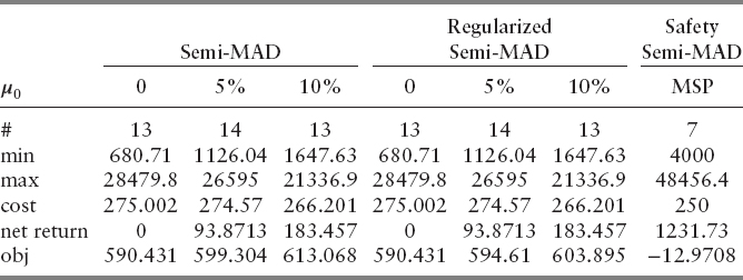
Tables 8.5 and 8.6 provide the same results shown in Table 8.4 for the PFC and the PCMC structures, respectively.
One may notice that the semi-MAD model in the coherent (safety) form, even with proportional transaction costs, builds portfolios with an extremely low level of diversification and high expected return. Therefore, the introduction of fixed transaction costs or minimum charge transaction costs does not affect results of this model. On the other hand, in the standard semi-MAD model and its regularized version, introducing fixed (minimum) charges into the transaction costs schemes decreases the portfolio diversification while still keeping it at a reasonable level. Moreover, in comparison to the standard semi-MAD model, the regularized semi-MAD model even for low net return requirements generates higher expected returns, while not increasing remarkably the risk level. This model seems to be very attractive for portfolio optimization with transaction costs including fixed or minimum charges.
TABLE 8.4 Computational Results: Pure Proportional Cost Structure with cj = 0.25 percent for all j ∈ N.
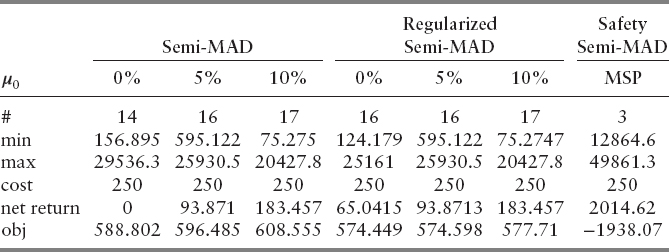

TABLE 8.6 Computational Results: Proportional Cost with Minimum Charge Structure with Fixed Cost Equal to 10 euros for a Minimum Charge up to 4,000 euros and 0.25% Proportional Cost for Larger Values of Capital.
CONCLUSIONS
In this chapter, we analyze the portfolio optimization problem with transaction costs by classifying them in variable and fixed costs. Past and recent literature on the topic has been surveyed. We analyze in detail the most common structures of transaction costs and the different manners to model them in portfolio optimization. The introduction of transaction costs may require the use of binary variables. For this reason, we focus on a risk measure that gives rise to a linear model, namely the mean semi-absolute deviation (semi-MAD).
We provide an example that shows how the portfolio optimization with transaction costs may lead to discontinuous efficient frontier and therefore a non-unique solution when minimizing the risk under a required expected return. This result motivates the introduction of a regularization term in the objective function in order to guarantee the selection of an efficient portfolio (regularized semi-MAD).
Finally, we run some simple computational results on a small set of securities to compare three simplified cost structures (pure proportional cost, pure fixed cost, proportional cost with minimum charge) when using three different objective functions: the semi-MAD in both the risk and safety form and the regularized semi-MAD. In the experimental analysis, we focus on costs inserted in the return constraint as more popular and better suited for absolute risk-minimization models. Results show how the regularized semi-MAD model even for low net return requirements generates higher expected returns while not increasing remarkably the risk level, thus resulting as an attractive model for portfolio optimization with transaction costs including fixed or minimum charges.
APPENDIX
In the following we show the main calculations behind the example reported in the fifth section of the chapter, “Non-unique Minimum Risk Portfolio.” The example shows how the portfolio optimization considering proportional transaction costs with minimum charge may lead to a discontinuous efficient frontier and therefore to a non-unique solution when minimizing the risk under a required expected return.
Feasibility of Portfolios (x1, x2, 0)
If x1 ≤ 5000 = 0.5C, then μ(x1, x2, 0)100 = 15.67x1 + 15.07(C − x1) − 0.5C − 1.0(C − x1) = 1.60x1 + 13.57C. Hence, μ(x1, x2, 0)100 ≥ 14C for any 43/160C ≤ x1 ≤ 0.5C.
If x1 ≥ 5000 = 0.5C, then μ(x1, x2, 0)100 = 15.67x1 + 15.07(C − x1) − 1.0x1 − 0.5C = − 0.40x1 + 14.57C. Hence, μ(x1, x2, 0)100 ≥ 14C for any 0.5C ≤ x1 ≤ C.
Finally, feasibility for 43/160C ≤ x1 ≤ C.
Feasibility of Portfolios (x1, 0, x3)
If x1 ≤ 5000 = 0.5C, then μ(x1, 0, x3)100 = 15.67x1 + 14.92(C − x1) − 0.5C − 1.0(C − x1) = 1.75x1 + 13.42C. Hence, μ(x1, 0, x3)100 ≥ 14C for any 58/175C ≤ x1 ≤ 0.5C.
If x1 ≥ 5000 = 0.5C, then μ(x1, 0, x3)100 = 15.67x1 + 14.92(C − x1) − 1.0x1 − 0.5C = − 0.25x1 + 14.42C. Hence, μ(x1, 0, x3)100 ≥ 14C for any 0.5C ≤ x1 ≤ C.
Finally, feasibility for 58/175C ≤ x1 ≤ C.
Infeasibility of Portfolios (0, x2, x3)
If x2 ≤ 5000 = 0.5C, then μ(0, x2, x3)100 = 15.07x2 + 14.92(C − x2) − 0.5C − 1.0(C − x2) = − 13.85x2 + 13.42C. Hence, μ(0, x2, x3)100 ≥ 14C for no x2 ≤ 0.5C.
If x2 ≥ 5000 = 0.5C, then μ(0, x2, x3)100 = 15.07x2 + 14.92(C − x2) − 1.0x2 − 0.5C = − 0.85x2 + 14.42C. Hence, μ(0, x2, x3)100 ≥ 14C needs 0.5C ≤ x2 ≤ 42/85C and there is no such x2.
Finally, no feasibility for any 0 ≤ x2 ≤ C.
Infeasibility of Portfolios (x1, x2, x3)
If x1 ≤ 5000 = 0.5C, then μ(x1, x2, x3)100 < 15.67x1 + 15.07(C − x1) − 1.5C = 0.60x1 + 13.57C. Hence, μ(x1, x2, x3)100 ≥ 14C for no x1 ≤ 0.5C.
If x1 ≥ 5000 = 0.5C, then μ(x1, x2, x3)100 < 15.67x1 + 15.07(C − x1) − 1.0x1 − 1.0C = − 0.40x1 + 14.07C. Hence, μ(x1, x2, x3)100 ≥ 14C for no x1 ≥ 0.5C.
Finally, no feasibility for any 0 ≤ x1 ≤ C.
REFERENCES
Adcock, C. J., and N. Meade, 1994. A simple algorithm to incorporate transactions costs in quadratic optimisation. European Journal of Operational Research 79: 85–94.
Angelelli, E., R. Mansini, and M. G. Speranza, 2008. A comparison of MAD and CVaR models with real features. Journal of Banking and Finance 32: 1188–1197.
_________. 2012. Kernel Search: A new heuristic framework for portfolio selection. Computational Optimization and Applications 51: 345–361.
Arnott, R. D., and W. H. Wagner. 1990. The measurement and control of trading costs. Financial Analysts Journal 46: 73–80.
Baule, R. 2010. Optimal portfolio selection for the small investor considering risk and transaction costs. OR Spectrum 32: 61–76.
Beasley, J. E., N. Meade, and T.-J. Chang. 2003. An evolutionary heuristic for the index tracking problem. European Journal of Operational Research 148: 621–643.
Bertsimas, D., and R. Shioda. 2009. Algorithm for cardinality-constrained quadratic optimization. Computational Optimization and Applications 43: 1–22.
Best, M. J., and J. Hlouskova. 2005. An algorithm for portfolio optimization with transaction costs. Management Science 51: 1676–1688.
Brennan, M. J. 1975. The optimal number of securities in a risky asset portfolio when there are fixed costs of transacting: Theory and some empirical results. Journal of Financial and Quantitative Analysis 10: 483–496.
Chang, T.-J., N. Meade, J. E Beasley, and Y. M. Sharaia. 2000. Heuristics for cardinality constraint portfolio optimisation. Computers and Operations Research 27: 1271–1302.
Chen, A. H., F. J. Fabozzi, and D. Huang. 2010. Models for portfolio revision with transaction costs in the mean-variance framework. Chapter 6 in Handbook of Portfolio Construction, John B. Guerard, Jr., Ed., Springer: 133–151.
Chen, A. H., F. C. Jen, and S. Zionts. 1971. The optimal portfolio revision policy. Journal of Business 44: 51–61.
Chiodi, L., R. Mansini, and M. G. Speranza. 2003. Semi-absolute deviation rule for mutual funds portfolio selection. Annals of Operations Research 124: 245–265.
Crama, Y., and M. Schyns. 2003. Simulated annealing for complex portfolio selection problems. European Journal of Operational Research 150: 546–571.
Guastaroba, G., R. Mansini, and M. G. Speranza. 2009. Models and simulations for portfolio rebalancing. Computational Economics 33: 237–262.
Jacob, N. L. 1974. A limited-diversification portfolio selection model for the small investor. Journal of Finance 29: 847–856.
Johnson, K. H., and D. S. Shannon. 1974. A note on diversification and the reduction of dispersion. Journal of Financial Economics 1: 365–372.
Kellerer, H., R. Mansini, and M. G. Speranza. 2000. Selecting portfolios with fixed cost and minimum transaction lots. Annals of Operations Research 99: 287–304.
Konno, H., K. Akishino, and R. Yamamoto. 2005. Optimization of a long-short portfolio under non convex transaction cost. Computational Optimization and Applications 32: 115–132.
Konno H., and R. Yamamoto 2005. Global optimization versus integer programming in portfolio optimization under nonconvex transaction costs. Journal of Global Optimization 32: 207–219.
Konno, H., and H. Yamazaki. 1991. Mean–absolute deviation portfolio optimization model and its application to Tokyo stock market. Management Science 37: 519–531.
Konno, H., and A. Wijayanayake. 2001. Portfolio optimization problem under concave transaction costs and minimal transaction unit constraints. Mathematical Programming 89: 233–250.
Krejić, N., M. Kumaresan, and A. Roznjik. 2011. VaR optimal portfolio with transaction costs. Applied Mathematics and Computation 218: 4626–4637.
Le Thi, H. A., M. Moeini, and T. Pham Dinh. 2009. DC programming approach for portfolio optimization under step increasing transaction costs. Optimization: A Journal of Mathematical Programming and Operations Research 58: 267–289.
Levy, H. 1978. Equilibrium in an imperfect market: A constraint on the number of securities in the portfolio. American Economic Revue 68: 643–658.
Lobo, M. S., M. Fazel, and S. Boyd. 2007. Portfolio optimization with linear and fixed transaction costs. Annals of Operations Research 152: 341–365.
Mansini, R., W. Ogryczak, and M. G. Speranza. 2003a. LP solvable models for portfolio optimization: A classification and computational comparison. IMA Journal of Management Mathematics 14: 187–220.
_________. 2003b. On LP solvable models for portfolio selection. Informatica 14: 37–62.
_________. 2007. Conditional value at risk and related linear programming models for portfolio optimization. Annals of Operations Research 152: 227–256.
_________. 2014. Twenty years of linear programming based portfolio optimization. European Journal of Operational Research 234 (2): 518–535.
Mansini, R., and M. G. Speranza. 1999. Heuristic algorithms for the portfolio selection problem with minimum transaction lots. European Journal of Operational Research 114: 219–233.
_________. 2005. An exact approach for portfolio selection with transaction costs and rounds. IIE Transactions 37: 919–929.
Markowitz, H. M. 1952. Portfolio selection, Journal of Finance 7: 77–91.
_________. 1959. Portfolio selection: Efficient diversification of investments. New York: John Wiley & Sons.
Mao, J. C. T. 1970. Essentials of portfolio diversification strategy. Journal of Finance 25: 1109–1121.
Mitchell J. E., and S. Braun. 2013. Rebalancing an investment portfolio in the presence of convex transaction costs, including market impact costs. Optimization Methods and Software 28: 523–542.
Ogryczak, W., and A. Ruszczyński. 1999. From stochastic dominance to mean–risk models: Semideviations as risk measures. European Journal of Operational Research 116: 33–50.
Patel, N. R., and M. G. Subrahmanyam. 1982. A simple algorithm for optimal portfolio selection with fixed transaction costs. Management Science 38: 303–314.
Speranza, M. G. 1993. Linear programming models for portfolio optimization. Finance 14: 107–123.
Williams, H. P. 2013. Model building in mathematical programming. 5th ed. Chichester: Wiley,
Woodside-Oriakhi, M., C., Lucas, and J. E. Beasley. 2013. Portfolio rebalancing with an investment horizon and transaction costs. Omega 41: 406–420.
Xue, H.-G., C.-X. Xu, and Z.-X. Feng. 2006. Mean-variance portfolio optimal problem under concave transaction cost. Applied Mathematics and Computation 174: 1–12.
Yoshimoto, A. 1996. The mean-variance approach to portfolio optimization subject to transaction costs. Journal of Operations Research Society of Japan 39: 99–117.
Young, M. R. 1998. A minimax portfolio selection rule with linear programming solution. Management Science 44: 173–183.