CHAPTER 3

Nonperforming Loans in the Bank Production Technology

Hirofumi Fukuyama

Fukuoka University

William L. Weber

Southeast Missouri State University

INTRODUCTION

Nonperforming loans are an undesirable by-product of the loan production process for financial institutions. Although collateral requirements can substitute for a borrower's lower probability of repayment (Saunders and Cornett 2008), financial institutions must still incur a charge when borrower's default. However, any attempt to eliminate nonperforming loans to zero would likely require financial institutions to employ large amounts of inputs to monitor borrowers or would require financial institutions to forgo some profitable lending. Both of these alternatives are likely inefficient. Instead, since bank owners choose the level of risk they wish to undertake (Hughes, Lang, Mester, and Moon, 1996), financial institutions should be willing to accept nonperforming loans up to the point where the lost income (including principal) on the marginal nonperforming loan is just offset by the reduced monitoring costs or by the increased interest income on the loan portfolio. In fact, policies that promote bank competition by reducing entry restrictions have the effect of reducing loan losses as well as the operating costs of production (Jayaratne and Strahan, 1998). Such competition can also be an effective means of weeding out managers who are weak at originating and monitoring the loan portfolio (Berger and Mester, 1997).

Many researchers have incorporated nonperforming loans into the financial institution production technology in measuring managerial performance and the shadow price of nonperforming loans, and in this chapter we focus our attention on studies that have examined Japanese bank performance. In addition, we present a new model that is capable of estimating prices for desirable outputs such as loans and securities investments and the price or charge of undesirable outputs such as nonperforming loans. Our method is grounded in duality theory and employs the directional output distance function measured in cost space. We also simulate how managers can use the estimated directional output distance function to minimize nonperforming loans by optimally reallocating their budgets over time. Here, our idea is that bank managers might want to forgo expenditures on inputs in one period so that larger amounts of inputs can be purchased in a different period.

We apply our method to 101 Japanese city and regional banks that operated in fiscal years 2008 to 2012. The Japanese fiscal year starts on April 1 and ends on March 31 of the subsequent year. We choose the years 2008 to 2012, as those years comprise the most recent available five-year span of data. In the next section, we provide a review of research measuring Japanese bank performance that incorporates nonperforming loans in the production technology. The next section presents our method used to measure performance and recover the prices of the desirable outputs produced by financial institutions as well as the undesirable outputs consisting of nonperforming loans. We then present the data and estimates of regional bank performance and the prices of the various outputs. In addition, we show how bank managers can use the parameter estimates of the directional output distance function to optimally reallocate spending on inputs and the desirable outputs so as to minimize the sum of nonperforming loans over the five-year period.

SELECTIVE LITERATURE REVIEW

Distance Functions

The reciprocal of the Shephard (1970) output distance function gives the maximum proportional expansion in all outputs that can be feasibly produced given inputs. The output distance function can be estimated using data envelopment analysis (DEA)—a set of mathematical programming techniques developed by Charnes, Cooper, and Rhodes (1978) and Banker, Charnes, and Cooper (1984)—which have been used by numerous researchers to estimate bank efficiency. Berger and Humphrey (1997) and Fethi and Pasiouras (2013) provide extensive surveys of financial institution performance using DEA. Shephard distance functions can also be estimated parametrically using the deterministic linear programming method of Aigner and Chu (1968) or using stochastic frontier methods.

When nonperforming loans are accounted for in the bank production technology, the measurement of bank performance is complicated by the fact that bank managers typically want to simultaneously expand desirable outputs and contract undesirable outputs. Unfortunately, Shephard output distance functions expand both desirable and undesirable outputs. As an alternative to Shephard output distance function, the directional distance function can be used to measure performance. Chambers, Chung, and Färe (1996) extended Luenberger's (1992; 1995) benefit function used in consumer theory to derive the directional input distance function. Luenberger (1995) proposed a more general shortage function, which Chambers, Chung, and Färe (1998) adapted and termed the directional technology distance function. The last obvious extension is the directional output distance function, which gives the maximum expansion in desirable outputs and simultaneous contraction in undesirable outputs. Färe and Grosskopf (2000) provide further discussion of these directional distance functions.

Shadow Prices of Nonperforming Loans

To estimate the Shephard output distance function, the translog functional form has enjoyed widespread use in parametric estimation of efficiency (Färe, Grosskopf, Lovell, and Yaisawarng 1993; Coggins and Swinton 1996; Swinton 1998) and shadow prices of undesirable outputs. However, the output distance function expands both desirable outputs and undesirable outputs to the production possibility frontier, whereas most managers are concerned with expanding desirable outputs and contracting undesirable outputs. Although the directional output distance functions can satisfy these criteria, Chambers (1998) suggests a quadratic form as a second-order approximation to the true, but unknown function. The quadratic form can be parameterized to satisfy the translation property, whereas the translog form can only be parameterized to satisfy homogeneity.

Although DEA can be used to estimate the directional output distance function and recover the shadow price of nonperforming loans, the directional output distance function estimated via DEA is not twice differentiable (Färe, Grosskopf, and Weber, 2006), resulting in a situation where there may be a range of shadow price ratios that support an observed frontier combination of desirable and undesirable outputs. Instead, researchers have employed twice differentiable functional forms such as the quadratic to estimate the directional output distance function. Färe, Grosskopf, Noh, and Weber (2005) exploited the duality between the directional output distance function and the revenue function to recover the shadow prices of undesirable outputs. They illustrated their method with an application to the U.S. electric utility industry by treating sulfur dioxide emissions as an undesirable output. Similarly, Färe, Grosskopf, and Weber (2006) treated human risk–adjusted leaching and runoff of pesticides in the U.S. agricultural industry as two undesirable outputs and estimated their shadow prices. Fukuyama and Weber (2008a; 2008b) estimated the shadow price of nonperforming loans for Japanese banks using a directional output distance function with estimates from both DEA and a quadratic functional form. They found significant differences in the distributions of shadow prices estimated by DEA and by the quadratic form.

Japanese Bank Efficiency

Several studies have examined the efficiency of Japanese banks. Kasuya (1986) estimated a translog cost function for 13 Japanese city banks and 64 Japanese local banks during the period 1975–1985. Using bank revenues from loans and other activities as the two bank outputs, Kasuya found significant scope economies for city banks and some evidence of scope economies for local banks during the latter part of the period. In addition, Kasuya found scale economies for both city and local banks. Fukuyama (1993) decomposed overall technical efficiency into pure technical efficiency and scale efficiency for Japanese banks operating in 1992 and found that the gains to be realized from enhanced pure technical efficiency are more than the scale efficiency gains. Furthermore, Fukuyama found a positive relation between pure technical efficiency and bank assets. Fukuyama (1995) used DEA to estimate the Malmquist indexes of productivity change, efficiency change, and technological change for Japanese banks during 1989–1991, which corresponds to the years before and after the collapse of the Japanese real estate and stock market bubbles.

Miyakoshi and Tsukuda (2004) estimated a stochastic frontier model and found regional disparities in technical efficiency among regional banks similar to Fukuyama's (1993) finding on scale economies. Fukuyama and Weber (2005) estimated the potential gains in earnings and found that those earnings could be expanded by 16 to 25 percent from an optimal reallocation of physical inputs. Harimaya (2004) estimated technical efficiency and cost efficiency and found that cooperative Shinkin banks with a lower ratio of costs to deposits exhibit greater technical efficiency. Liu and Tone (2008) measured Japanese banking efficiency during 1997 to 2001 and found that banks appeared to be “learning by doing,” as bank efficiency increased during the period.

Several researchers have taken into account risk factors such as nonperforming loans in their analyses of Japanese bank efficiency. Using Japanese bank data from 1992 to 1995, Altunbus et al. (2000) showed that bank scale economies are likely overstated if loan quality and bank risk-taking are not accounted for. Drake and Hall (2003) found substantial inefficiency and clear evidence of scale economies for small banks and diseconomies of scale for large city banks when nonperforming loans are ignored during 1992 to 1995. However, after controlling for nonperforming loans, the researchers found the extent of scale economies for small banks and scale diseconomies for large banks to be reduced. Hori (2004) controlled for nonperforming loans and used DEA to estimate cost efficiency for Japanese banks in 1994. He concluded that the average regional banks could have reduced operating costs by about 20 percent if they were able to minimize costs. In addition, he found the primary cause of cost inefficiency for regional banks to be pure technical inefficiency—the overuse of all inputs—rather than allocative inefficiency due to an inappropriate mix of inputs. Fukuyama and Weber (2008a, 2008b) estimated efficiency, technological change, and shadow prices for nonperforming loans for Japanese commercial banks and Shinkin banks during 2002 to 2004 and concluded that regional banks experienced faster technological progress than Shinkin banks. Fukuyama and Weber (2009) controlled for nonperforming loans and bank risk in their DEA model and found that the revenue-constrained Luenberger productivity indicator decreased during 2000 to 2001 and 2003 to 2006.

Drake, Hall, and Simper (2009) estimated a slacks-based efficiency measure and found evidence that significant differences in sample efficiency estimates, the dispersion of efficiency, temporal variations, and mean efficiency estimates across sectors depended on how researchers defined bank inputs and outputs. Perhaps one of the greatest specification issues concerns the treatment of deposits, which some researchers have specified as an output and other researchers have specified as an input. To address the specification of deposits issue, Fukuyama and Weber (2010) developed a network bank efficiency model, and Fukuyama and Weber (2013, 2014) extended it into a dynamic-network framework. The authors proposed a two-stage network technology where banks use labor, physical capital, and equity capital to produce deposits in a first stage of production, with those deposits then used as an input in the second stage of production to produce the final desirable outputs of loans and securities investments along with a jointly produced undesirable output in the form of nonperforming loans. The models take on a dynamic aspect in that the nonperforming loans generated in one period become an undesirable input that constrains what banks can produce in a subsequent period. These dynamic network models were applied to Japanese banks operating from 2006 to 2010. In conclusion, the implication of these studies is that incorporation of nonperforming loans in the efficiency analysis for Japanese banks is of great significance.

METHOD

Recent work by Färe, Grosskopf, Sheng, and Sickles (2012) and Cross, Färe, Grosskopf, and Weber (2013) exploited the duality between the directional input distance function and the cost function to recover the prices of nonmarket output characteristics. Their work is related to the hedonic pricing method of Rosen (1974), who showed in a theoretical model that the implicit prices of a bundle of product characteristics can be recovered such that the relative prices equal the consumer's marginal rate of substitution between the characteristics and the producer's marginal rate of transformation between the characteristics. We extend the work of Färe et al. (2012) and Cross et al. (2013) to recover output prices using a directional output distance function defined in cost space.

We model the production technology using the directional output distance function in cost space. Banks face a budget, c, that allows them to produce desirable outputs and jointly produced undesirable outputs . The output correspondence (production possibility set) is given as

The production possibility set P(c) gives the various combinations of desirable and undesirable outputs that can be produced at a given budget or cost and has the following properties:

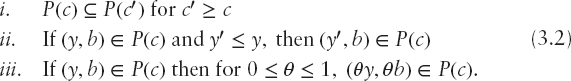
Property (3.2)i means that the output correspondence does not shrink for producers that have a larger budget. Similarly, (3.2)ii corresponds to strong disposability of desirable outputs. Property (3.2)iii imposes weak disposability for the jointly produced desirable and undesirable outputs. That is, holding the budget constant, the opportunity cost of reducing the undesirable outputs is that less of the desirable outputs can be produced.

We use the directional output distance function to represent the production possibility set. This function scales outputs to the frontier of the production technology along the directional vector g_y = (g_y1, …, g_yM) and g_b = (g_b1, …, g_bJ). The directional output distance function is defined as

The directional distance function finds the maximum additive expansion in outputs for the given directional vectors. We want to choose a directional vector that gives credit to producers that simultaneously expand desirable outputs and contract undesirable outputs. Therefore, we choose a non-negative directional vector for desirable outputs and a nonpositive directional vector for undesirable outputs: g_y ≥ 0 and g_b ≤ 0. Different directional vectors can be chosen, depending on the objectives of the manager or policy maker. A directional vector of g_y = (y₁, y₂, …, y_M) and g_b = (−b₁, −b₂, …, −b_J) would give the simultaneous maximum proportional expansion in desirable outputs and proportional contraction in undesirable outputs. A directional vector of g_y = (1, 1, …, 1) and g_b = (−1, −1, …, −1) would give the simultaneous maximum unit expansion in desirable outputs and unit contraction in undesirable outputs. If managers are interested in finding the maximum contraction in undesirable outputs holding desirable outputs constant, then g_y = (0, 0, …, 0) and g_b < 0 for undesirable outputs should be chosen. If managers are interested in finding the maximum expansion in desirable outputs holding undesirable outputs constant, then a choice of g_b = (0, 0, …, 0) and g_y > 0 would be appropriate.

When , the producer is on the frontier of P(c); it cannot simultaneously expand desirable outputs and contract undesirable outputs given the budget with which to hire inputs. These producers are technically efficient for the given directional vectors, g_y and g_b. Inefficient producers have with higher values indicating greater inefficiency.

The directional distance function inherits its properties from the production possibility set:

These properties include feasibility (3.4)i, monotonicity conditions (3.4)ii–iv, the translation property (3.4)v, and concavity (3.4)vi.

We follow Färe and Primont (1995) and exploit the duality between the revenue function and the directional output distance function to obtain the prices that support the outputs on the production possibility frontier. Let represent the desirable output price vector and represent the undesirable output price vector. The revenue function takes the form:

In (3.5), firms gain revenue of p for every unit of desirable output they produce but must also pay a charge of q for every unit of undesirable output they produce.

One way of recovering the shadow price of the undesirable output is by using the first-order conditions associated with the constrained maximization of 3.5. The first-order conditions imply that the ratio of prices equal the ratio of derivatives of the distance function with respect to the outputs:

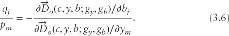
Given knowledge of a single marketed output price, say p_m, the shadow price of the nonmarketed undesirable output, q_j, can be recovered using (3.6). However, this shadow pricing method requires the researcher to observe at least one marketed output price. In what follows below, we recover all prices without knowledge of a single market price.

Using the duality between the directional output distance function and the revenue function, we can write

In words, (3.7) says that actual revenues (py − qb) are equal to maximum revenues R(c, p, q) less a deduction for producing inefficient amounts of the desirable outputs in the amount of and a further deduction (since g_b < 0) for overproducing the undesirable outputs in the amount of . Taking the gradient function of (3.7) with respect to desirable outputs and then again with respect to undesirable outputs yields

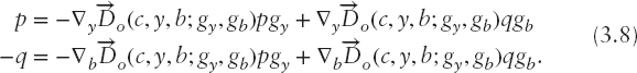
Collecting terms in (3.8) yields

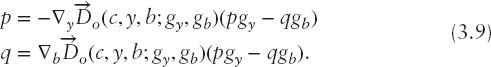
Multiplying the first equation in (3.9) by the desirable output vector y and the second equation in (3.9) by the undesirable output vector b yields

Subtracting the second equation in (3.10) from the first equation in (3.10) yields

Since (pg_y − qg_b) is positive and since c = py − qb is also positive, it must be the case that the term in brackets on the left-hand side of (3.11) is negative:

Solving (3.11) for (pg_y − qg_b) yields

Finally, substituting (3.13) into (3.9) yields the pricing formulas for the desirable and undesirable outputs:

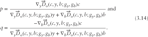
Since the denominator of (3.14) is negative via (3.12), and the monotonicity properties of the directional output distance function imply that and , the pricing formulae (3.14) yield p ≥ 0 and q ≥ 0. The most significant result of (3.14) is that we do not need price information in contrast to the shadow pricing methods of Fukuyama and Weber (2008a; 2008b).

To implement the pricing formulae (3.14), we need to choose a functional form for the directional output distance function. Although DEA can be used to estimate dual shadow prices, DEA provides only a first-order approximation to the true but unknown production technology. In contrast, the translog functional form has been used as a second-order approximation to a true but unknown technology that can be estimated via Shephard output or input distance functions. However, the Shephard output distance function seeks the maximum expansion of both desirable and undesirable outputs. Since we want to give credit to banks that successfully expand desirable outputs and contract undesirable outputs, we choose a quadratic form for the directional output distance function. Although the translog form is suitable for modeling the homogeneity property of Shephard distance functions, the directional output distance function has the translation property that can be modeled using a quadratic form.

Given k = 1, …, K firms (banks) that produce in t = 1, …, T periods, the quadratic directional output distance function takes the form

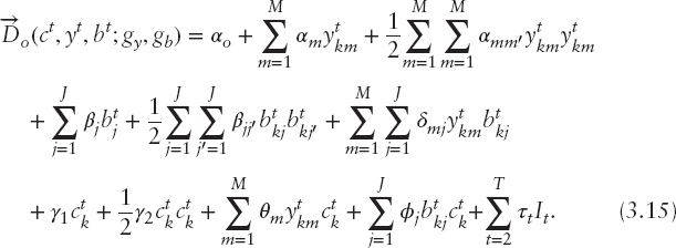
We allow for technological progress/regress by defining binary indicator variables, I_t, for each of the t = 2, …, T periods. For a given observation on budget, desirable outputs, and undesirable outputs (c, y, b), the sign of the coefficients τ_t tells us whether the distance of the observation to the period t frontier (t ≠ 1) is further (τ_t > 0) or closer (τ_t < 0) than it is to the frontier in period t = 1. Positive values for τ_t indicate technological progress and negative values indicate technological regress. We impose symmetry on the cross-product effects, α_mm′ = α_m′m and β_jj′ = β_j′j. The translation property is imposed by the following coefficient restrictions: , , m = 1, …, M, , j = 1, …, J, and . Finally, the directional output distance function must be concave in outputs. Let the matrix 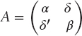be the matrix of second-order and cross-product terms for the desirable and undesirable outputs, where , , 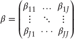and . For the directional output distance function to satisfy concavity, the matrix A must be negative semi-definite (Lau 1978, Morey 1986).

To estimate the directional distance function, we use the deterministic method of Aigner and Chu (1968). This method chooses coefficients so as to minimize the distance of each observation to the production possibility frontier:

In (3.4) we stated the properties of the directional output distance function and these properties are incorporated in (3.16). That each observation be feasible is given by the restriction (3.16)viii. The monotonicity conditions are incorporated in (3.16)iii, iv, and v. Restrictions corresponding to the translation property are given in (3.16)ii. The symmetry conditions for the quadratic form are given by (3.16)i and concavity is given by (3.16)vi. We impose concavity on the directional output distance function by decomposing the matrix A into its Cholesky factorization and imposing constraints on the Cholesky values of A.¹ The conditions in (3.16)vii ensure that the desirable and undesirable output prices are non-negative.

EMPIRICAL APPLICATION

Data Source and Data Description

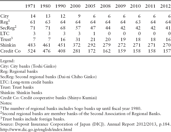
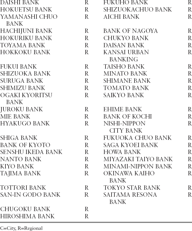
Mergers, acquisitions, and regulatory closures have led to consolidation in the Japanese banking industry, and the trends among various bank types can be seen in Table 3.1. The data for Japanese banks were obtained via the Nikkei Financial Quest, which is an online data retrieval system that provides firm-level financial data. To estimate our model, we use pooled data on 101 banks during the five fiscal years of 2008 to 2012. The 101 banks include five city banks and 96 regional banks, which comprise first regional banks and second regional banks. In 2008 there were 64 first regional banks and 44 second regional banks. From 1971 to 2008, the number of second regional banks fell from 71 to 44 and by 2012 (the last year of our sample), the number of second regional banks had fallen to 41. Because of missing data, we deleted six regional banks from our sample: Tokyo Tomin Bank, Shinsei Bank, Kumamoto, Seven Bank, Tokushima Bank, Kagawa Bank, and Shinwa Bank. The bank names used in this study are provided in the Appendix 3.1.

Berger and Humphrey (1992) provide an overview of the various ways researchers have defined bank outputs and inputs. The asset approach of Sealey and Lindley (1977) includes bank assets such as loans and securities investments as the outputs of bank production, while the various deposit liabilities are inputs. In contrast to the asset approach, Barnett and Hahm (1994) assume that banks produce the nation's money supply using a portfolio of loans and securities investment. The user cost approach of Hancock (1985) defines bank outputs as activities that add significantly to revenues and bank inputs as activities where there is an opportunity cost of production.

We follow the asset of approach of Sealey and Lindely (1977) in defining bank outputs. This approach has also been used by Fukuyama and Weber (2008a; 2008b; 2013; 2014) in studying Japanese bank efficiency. We assume that Japanese banks produce two desirable outputs and one undesirable jointly produced output by hiring inputs using their fixed budget (c). The budget (c = value of the inputs) equals total bank expenditures. In turn, total bank expenditures equal the sum of personnel expenditures, nonpersonnel expenditures, and interest expenditures. These expense categories are associated with the physical inputs of labor, physical capital, and raised funds.

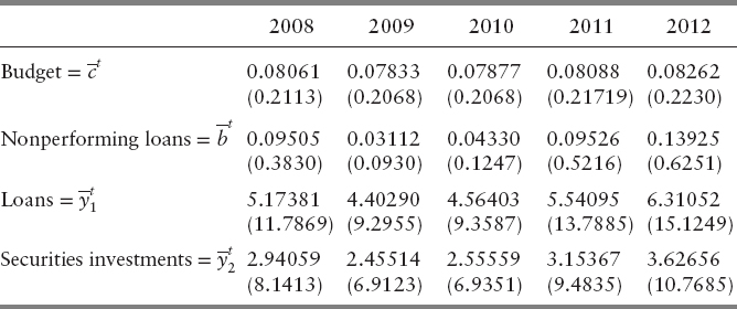
Each of the outputs and the budget are in real terms, having been deflated by the Japanese GDP deflator. The desirable outputs are total loans (y₁) and securities investments (y₂). Financial Quest documents four categories of nonperforming loans: (1) risk management loans, which equal the sum of loans to bankrupt borrowers; (2) nonaccrual delinquent loans; (3) loans past due for three months or more; and (4) restructured loans. Risk management loans are items under banks accounts reported in the statement of risk-controlled loans. The sum of the four categories of nonperforming loans equals total nonperforming loans, which we take to be the jointly produced undesirable output (b₁).

Table 3.2 reports descriptive statistics for the pooled data. Total loans average 4.2 trillion yen and range from 0.16 trillion yen to 80.9 trillion yen. Securities investments average 2.4 trillion yen and range from 0.04 trillion yen to 71 trillion yen. Nonperforming loans average 0.11 trillion yen and range from 0.01 trillion yen to 0.21 trillion yen. As a percentage of total assets, nonperforming loans average 2.35 percent with a range from 0.5 percent to 5.2 percent. Nonperforming loans declined from 2.6 percent of total assets in 2008 to 2.2 percent of total assets in 2012. The average cost of production was 0.08 trillion yen, with the smallest regional bank incurring costs of only 0.004 trillion yen and the largest city bank incurring costs of 2.1 trillion yen.

Empirical Results

We estimate the quadratic directional output distance function for the directional scaling vectors, g_y = (y₁, y₂) = (4.189690, 2.374593), and g_b = b₁ = 0.110467, where y₁, y₂, b₁ are the averages of total loans, securities investments, and NPLs reported in Table 3.2. While we provided the descriptive statistics of the financial variables in Table 3.2 in millions of yen, our estimation of the directional output distance function is carried out in trillions of yen. The estimated directional output distance function multiplied by the directional vector gives the simultaneous contraction in nonperforming loans, and expansion in total loans and securities investments. That is, the expansion in the desirable outputs will equal and the simultaneous contraction in the undesirable output will equal . Since the directional vector equals the averages of the desirable and undesirable outputs, the directional distance function is the amount that the outputs will change as a proportion of the mean.

Table 3.3 reports the parameter estimates for the quadratic directional output distance function. The sum of all 101 banks’ inefficiencies over the five sample years equals 121.705.

One can easily check to see that the parameter estimates satisfy the translation property. For example, the first-order coefficients for the desirable and undesirable outputs multiplied by the directional vector must sum to negative one: α₁g_y1 + α₂g_y2 + β₁g_b1 = −1. Using the coefficients in Table 3.3 yields −0.1742 × 4.18969 − 0.0270 × 2.374593 + 1.8638 × (−0.110467) = −1. Similarly, the translation restrictions for the second-order and cross-product terms can be shown to be satisfied.

To measure technological change we evaluate . A positive value of this derivative means that holding the outputs and the budget constant, as time passes a bank, is further from the frontier, indicating technological progress. If the value is negative, then the bank exhibits technological regress. The estimated coefficients (τ₂ = 0.000 (2009), τ₃ = 0.003 (2010), τ₄ = 0.066 (2011), τ₅ = 0.109 (2012)) indicate that over time a given observation of outputs becomes further and further from the P(c) frontier.

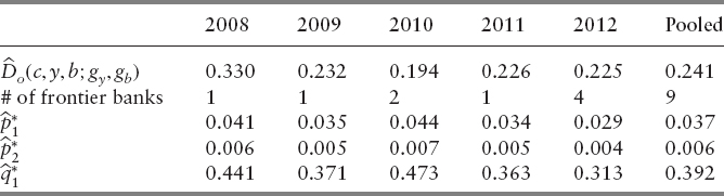
Table 3.4 presents the estimates of the directional output distance function, the number of frontier banks, and the prices for the two desirable outputs of loans and securities investments and the single undesirable output of nonperforming loans. Average inefficiency over the five-year period has a U-shape trending down from 0.33 in 2008 to 0.194 in 2010 and then rising slightly to 0.225 in 2012. For the five-year period, eight different banks² produce on the frontier with one bank on the frontier in 2008, 2009, and 2011, two banks on the frontier in 2010, and four banks on the frontier in 2012. Only one bank—Saitama Resona Bank—produced on the frontier in more than one year: 2011 and 2012.

The pooled price estimates for the desirable outputs average 3.7 percent for loans and 0.6 percent for securities investments. The price of loans reaches its maximum of 4.4 percent in 2010 and has a minimum of 2.9 percent in 2012. The price of securities investments ranges from 0.4 percent in 2012 to 0.7 percent in 2010. The charge on nonperforming loans averages 39.2 percent for the pooled sample and ranges from 47.3 percent in 2010 to 31.3 percent in 2012.

We further examine the estimates for a single bank, Tokyo Mitsubishi–UFJ Bank, which produced on the frontier in 2012. Tokyo Mitsubishi-UFJ bank is a large city bank that had costs of c = 1.534 trillion in 2012 and generated loans (y₁) equal to 80.9288 trillion yen, securities investments (y₂) equal to 70.3922 trillion yen, and nonperforming loans (b₁) equal to 1.7776 trillion yen. Its estimated prices in 2012 were p₁ = 0.01996, p₂ = 0.0056, and q₁ = 0.26743. Multiplying those prices by the respective outputs and summing yields revenues (and costs) of p₁y₁ + p₂y₂ − q₁b₁ = c = 0.01996 × 80.9288 + 0.0056 × 70.3922 − 0.26743 × 1.7776 = 1.534. Similar calculations hold for all other banks in all years.

Recent work by Färe, Grosskopf, Margaritis, and Weber (2012) investigated the issue of time substitution for producers. The goal of time substitution is to reallocate inputs or the budgets used to hire inputs across time so as to maximize production. The theoretical findings indicate that when there are increasing returns to scale, production should take place intensively in a single period and under conditions of decreasing returns to scale equal amounts of inputs should be employed in each period so as to maximize production. When technological progress occurs, firms should wait until later periods to use inputs, and when technological regress occurs, firms should use inputs earlier.

Here, we present a similar time substitution problem for Japanese banks. We use the parameter estimates of reported in Table 3.3 to simulate the effects of each bank optimally reallocating its budget c over time so as to minimize the sum of the undesirable output of nonperforming loans, while still producing a target level of the two desirable outputs. We choose the target for the desirable outputs to equal the actual output produced plus the estimated inefficiency in the output. That is, the target level of each output equals 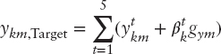, m = 1, 2. We use nonlinear programming to solve the following problem for each of the 101 banks:

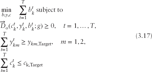
where equals the sum of bank k's costs over the five-year period. In this problem the choice variables are the amount to spend in each period, , and the amounts of the two desirable outputs, , and jointly produced undesirable output of nonperforming loans, , to produce each period. These variables are chosen so as to minimize the sum of nonperforming loans over the five-year period. The choices of , , and , m = 1, 2 must also be feasible. That is, the choices must satisfy in each year. We solve (3.17) for each of the 101 banks in our sample.

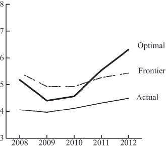
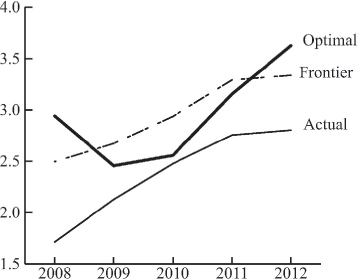
Table 3.5 presents the estimated optimal quantities for each period and Figures 3.1, 3.2, and 3.3 graph the optimal quantities of each output found as the solution to (3.17), the actual quantities, and the frontier quantities derived as and , where is the estimate of the directional output distance function from equation (3.16). Although the optimal quantities of the two desirable outputs summed over the five years equal the sum of the frontier quantities of the two desirable outputs and the sum of the optimal allocation of costs from (3.17) over the five years equals the sum of the actual costs over the five years, the optimal amount of nonperforming loans found as the objective function to (3.17) is less than the sum over the five years of the frontier amounts of nonperforming loans. The average amount of nonperforming loans is 0.11047 trillion yen. If banks were able to reduce inefficiency and produce on the frontier of the technology P(c), they would have average nonperforming loans of 0.08369 trillion yen. If the average bank were then able to optimally reallocate its budget across the five years, the average amount of nonperforming loans would be 0.08080 trillion yen.

The pricing problem given by (3.14) resulted in price estimates for the three outputs such that the value of the outputs equaled the cost of production. However, the price estimates typically varied for each bank in each year. Economic theory indicates that when relative prices vary across periods, firms can increase efficiency by reallocating production until the relative prices—the marginal rates of transformation—are equal in each period. The solution to (3.17) resulted in an allocation such that for each bank relative prices were equalized across the five periods. However, even after each individual bank reallocated across the five periods there was still some interbank variation in relative prices. Such a finding indicates that the banking system as a whole could further benefit by interbank reallocation of the budgets, with some banks expanding and some contracting until prices are equalized for all banks in all periods.

We also estimated (3.17) assuming that costs, nonperforming loans, and loans and securities investments should be discounted across time. We used a discount rate of 1 percent, which is the average yield on interest bearing liabilities among the banks in our sample. The results were largely the same as the undiscounted model, although a higher discount rates might cause larger differences.

SUMMARY AND CONCLUSION

Knowing the appropriate charge that must be borne for making a loan that becomes nonperforming provides important information to bank managers as they seek to determine the optimal bank portfolio. Although shadow pricing methods are well developed and can be used to recover charges for nonperforming loans, the method requires knowledge of one marketed output price and the marginal rate of transformation of outputs along a production frontier. In this paper, we presented a method that allows all prices to be recovered from a directional output distance function defined in cost space, which corresponds to the set of outputs that can be produced at a given cost. We estimated a quadratic directional output distance function using parametric methods and recovered prices for the desirable outputs of loans and securities investments and the charge on nonperforming loans for 101 Japanese banks during the period 2008 to 2012.

Our findings indicate that Japanese banks experienced technological progress during the period and that average bank inefficiency had a U-shaped trend, declining from 2008 to 2010, before rising slightly through 2012. We also found that the charge to be borne for nonperforming loans ranged averaged 0.39. We also used the estimates of the directional output distance function to simulate the effects of bank managers optimally reallocating their budgets across time. Actual nonperforming loans averaged 0.11047 trillion yen during the period. If bank managers were able to reduce inefficiency and produce on the production frontier nonperforming loans could be reduced to 0.083 trillion yen. Nonperforming loans could be reduced even further to 0.081 trillion yen if bank managers optimally allocated resources across time.

APPENDIX 3.1 BANK NAMES AND TYPE

REFERENCES

Aigner, D. J., and S. F. Chu. 1968. On estimating the industry production function. American Economic Review 58: 826–839.

Altunbas, Y., M. Liu, P. Molyneux, and R. Seth. 2000. Efficiency and risk in Japanese banking. Journal of Banking and Finance 24: 1605–1638.

Banker, R. D., A. Charnes, and W. W. Cooper. 1984. Some models for estimating technical and scale inefficiencies in Data Envelopment Analysis. Management Science, 30: 1078–1092.

Barnett, W., and J-H. Hahm. 1994. Financial firm production of monetary services: A generalized symmetric Barnett variable profit function. Journal of Business and Economic Statistics 12 (1): 33–46.

Berger, A. N., and D. B. Humphrey. 1992. Measurement and efficiency issues in commercial banking. In Output Measurement in the Service Industry, edited by Z. Griliches, 245–300, Chicago: University of Chicago Press.

_________. 1997. Efficiency of financial institutions: international survey and directions for future research. European Journal of Operational Research 98: 175–212.

Berger, A. N., and L. J. Mester. 1997. Inside the black box: What explains differences in the efficiencies of financial institutions? Journal of Banking and Finance 21 (7): 895–947.

Chambers, R. G. 1998. Input and output indicators. In Färe, R., Grosskopf, S., Russell, R. R. (eds.), Index Numbers: Essays in Honour of Sten Malmquist. Dordrecht: Kluwer Academic.

Chambers, R. G., Y. Chung, and R. Färe. 1996. Benefit and distance functions. Journal of Economic Theory 70 (2): 407–419.

Chambers, R. G., Y. Chung, and R. Färe. 1998. Profit, directional distance functions and Nerlovian efficiency. Journal of Optimization Theory and Applications 95(2): 351–364.

Charnes, A., W. W. Cooper, and E., Rhodes. 1978. Measuring the efficiency of decision-making units. European Journal of Operational Research 2(6): 429–444.

Coggins, J. S., and J. R. Swinton. 1996. The price of pollution: a dual approach to valuing SO₂ allowances. Journal of Environmental Economics and Management 30: 58–72.

Cross, R., R. Färe, S. Grosskopf, and W. L. Weber. 2013. Valuing vineyards: A directional distance function approach. Journal of Wine Economics 8 (1): 69–82.

Drake, L., and M. J. B. Hall. 2003. Efficiency in Japanese banking: An empirical analysis. Journal of Banking and Finance 27: 891–917.

Drake, L., M. J. B. Hall and R. Simper. 2009. Bank modeling methodologies: A comparative non-parametric analysis of efficiency in the Japanese banking sector. Journal of International Financial Markets, Institutions and Money 19 (1): 1–15.

Färe, R., and S. Grosskopf. 2000. Theory and application of directional distance functions. Journal of Productivity Analysis 13 (2): 93–103.

Färe, R., S. Grosskopf, C. A. K. Lovell, and S. Yaisawarng. 1993. Derivation of shadow prices for undesirable outputs: a distance function approach. The Review of Economics and Statistics, 374–380.

Färe, R., S. Grosskopf, D. Margaritis, and W. L. Weber 2012. Technological change and timing reductions in greenhouse gas emissions. Journal of Productivity Analysis 37: 205–216.

Färe, R., S. Grosskopf, D. W. Noh, and W. L. Weber. 2005. Characteristics of a polluting technology: Theory and practice. Journal of Econometrics 126: 469–492.

Färe, R., S. Grosskopf, C. Sheng, and R. Sickles. 2012. Pricing characteristics: An application of Shephard's dual lemma, mimeo.

Färe, R., S., Grosskopf, and W. L. Weber. 2006. Shadow prices and pollution costs in U.S. agriculture. Ecological Economics 1 (1): 89–103.

Färe, R., and D. Primont. 1995. Multi-Output Production and Duality: Theory and Applications. Norwell, MA: Kluwer Academic.

Fethi, M. D., and F. Pasiouras. 2013. Assessing bank efficiency and performance with operational research and artificial intelligence techniques: A survey. European Journal of Operational Research 204 (2): 189–198.

Fukuyama, H. 1993. Technical and scale efficiency of Japanese commercial banks: A non-parametric approach. Applied Economics 25: 1101–1112.

_________. 1995. Measuring efficiency and productivity growth in Japanese banking: a nonparametric frontier approach. Applied Financial Economics 5: 95–107.

Fukuyama, H., and W. L. Weber. 2005. Modeling output gains and earnings’ gains. International Journal of Information Technology and Decision Making 4 (3): 433–454.

_________. 2008a. Japanese banking inefficiency and shadow pricing. Mathematical and Computer Modeling 48 (11–12): 1854–1867.

_________. 2008b. Estimating inefficiency, technological change, and shadow prices of problem loans for Regional banks and Shinkin banks in Japan. The Open Management Journal, 1: 1–11.

_________. 2009. Estimating indirect allocative inefficiency and productivity change. Journal of the Operational Research Society 60: 1594–1608.

_________. 2010. “A slacks-based inefficiency measure for a two-stage system with bad outputs.” Omega: The International Journal of Management Science 38: 398–409.

_________. 2013. A dynamic network DEA model with an application to Japanese cooperative Shinkin banks. In: Fotios Pasiouras (ed.) Efficiency and Productivity Growth: Modeling in the Financial Services Industry. London: John Wiley & Sons, Chapter 9, 193–213.

_________. 2014. Measuring Japanese bank performance: A dynamic network DEA approach. Journal of Productivity Analysis.

Hancock, D. 1985. The financial firm: Production with monetary and nonmonetary goods. Journal of Political Economy 93: 859–880.

Harimaya, K. 2004. Measuring the efficiency in Japanese credit cooperatives. Review of Monetary and Financial Studies 21: 92–111 (in Japanese).

Hori, K. 2004. An empirical investigation of cost efficiency in Japanese banking: A nonparametric approach. Review of Monetary and Financial Studies 21: 45–67.

Hughes, J. P., W. Lang, L. J. Mester, and C-G. Moon. 1996. Efficient banking under interstate branching. Journal of Money, Credit, and Banking 28 (4): 1045–1071.

Jayaratne, J. and P. E. Strahan. 1998. Entry restrictions, industry evolution, and dynamic efficiency: Evidence from commercial banking. Journal of Law and Economics 41 (1): 239–274.

Kasuya, M. 1986. Economies of scope: Theory and application to banking. BOJ Monetary and Economic Studies 4: 59–104.

Lau, L. J. 1978. Testing and imposing monotonicity, convexity and quasi-convexity constraints. In M. Fuss and D. McFadden, eds. Production Economics: A Dual Approach to Theory and Applications volume 1. Amsterdam: North Holland.

Liu, J., and K. Tone. 2008. A multistage method to measure efficiency and its application to Japanese banking industry.” Socio-Economic Planning Sciences 42: 75–91.

Luenberger, D. G. 1992. Benefit functions and duality. Journal of Mathematical Economics 21: 461–481.

_________. 1995. Microeconomic Theory. Boston: McGraw-Hill.

Miyakoshi, T., and Y. Tsukuda. 2004. Regional disparities in Japanese banking performance. Review of Urban and Regional Development Studies, 16: 74–89.

Morey, E. R. 1986. An introduction to checking, testing, and imposing curvature properties: The true function and the estimated function. Canadian Journal of Economics 19 (2): 207–235.

Rosen, S. 1974. Hedonic prices and implicit markets: Product differentiation in pure competition. Journal of Political Economy 8(1): 34–55.

Saunders, A., and M. Cornett. 2008. Financial Institutions Management: A Risk Management Approach. 6th ed. New York: McGraw-Hill Irwin.

Shephard, R. W. 1970. Theory of Cost and Production Functions. Princeton: Princeton University Press.

Sealey, C., and J. T. Lindley. 1977. Inputs, outputs and a theory of production and cost at depository financial institutions, Journal of Finance, 33: 1251–1266.

Swinton, J. R. 1998. At what cost do we reduce pollution? Shadow prices of SO₂ emissions. The Energy Journal 19 (4): 63–83.