Chapter 5
Direct Current Machines
5.1. Introduction
The so-called “direct current machines” are electromechanical energy converters in which the electrical energy is exchanged with their environment (supply or load) under the form of direct voltages and currents. This is possible due to the brush-commutator systems which plays the part of a “mechanical rectifier”. That is the reason why these machines are sometimes called “commutator machines”.
Like all rotating machines, DC machines are reversible and can operate as a motor or as a generator (they are sometimes called “dynamos” in this case). However it can be noted that the development of power electronics, and particularly of diode and thyristor rectifiers, from the 1960s onwards, has gradually marginalized the use of DC generators. Today the generator function of these machines is restricted to the recovery of kinetic energy during braking and slowing down, we shall therefore focus this chapter on the motor mode.
5.2. Main notations
In the remainder of this chapter, we shall allot the index “1” to the field system, and the index “2” to the armature. We shall also set down:
– e: air-gap thickness;
– E: electromotive force;
– J: moment of inertia of all of the rotating parts;
– Li: self inductance of the winding i;
– M: mutual inductance between the field system and the armature;
– Ri: resistance of the winding i;
– U: supply voltage;
– μ0: free space permeability (μ0 = 4π 10–7 H/m);
– Ω: angular speed of the rotor;
– Γ: machine torque;
– ΓC: “load” torque.
5.3. DC machine structure
5.3.1. Constituents
Figure 5.1 represents a bipolar DC machine. It is composed of:
– a solid stator bearing a field system, usually a salient-pole system. It bears the field coil intended to produce the excitation magnetic field. Each pole is made of a core and of a pole shoe allowing the concentration of the field along the air-gap. For small machines, the excitation field coil is sometimes replaced by permanent magnets;
– a non-salient laminated rotor bearing the armature winding. The armature conductors are set down in slots and linked so that they make an unbroken winding fully closed on itself;
– a commutator rotating with the rotor and made of conductive segments insulated from one another. The armature conductors are linked to the commutator segments;
– fixed brushes rubbing on the commutator segments and making up the armature terminals (Figure 5.2).
Figure 5.1. Bipolar DC machine

The brush-commutator set allows the selection of the armature coils so that the “outward” conductors are separated from the “return” conductors by the stator interpolar axis (Figure 5.1). We shall demonstrate later on in this chapter that this spatial distribution of the currents is fixed during the rotation, and that the armature winding can be modeled by a fixed axis stationary coil.
Figure 5.2. Brushes-commutator set

Figure 5.3. Armature of a DC machine, 180 W, 960 rpm: a) commutator side, b) end windings side (ECA EN document)

Figures 5.3a and b show the rotor of a small DC machine. Note that the “useful” length of the conductors is quite small compared to the overall length because of the size of the end winding and of the commutator.
Figure 5.4 shows the brushes and the commutator of a four-pole machine. Note the important length of the commutator segments; the brush-commutator contact surface indeed has to be enough in order to limit the current density going through them.
Figure 5.4. Brush-commutator set. Note the important length of the commutator segments. To allow a good contact quality, the brushes are divided in several parts (ECA EN document)

Figure 5.5 shows the arrangement of the outward and return conductors in the armature slots of a four-pole machine.
Figure 5.5. Armature of a four-pole machine

Figure 5.6. Field lines. Bipolar machine

5.3.2. Analysis of the field winding
Figure 5.6 shows the field lines obtained when only the field winding is supplied. These lines rotate around excitation currents; they cross the air-gap, then the rotor, and finally close through the stator. We can observe that on a first approximation, these lines only cross the part of the air-gap, of small thickness e, located under the pole shoes.
Figure 5.7a shows the variation of the normal flux density along the air-gap. The origin θ = 0 corresponds to the interpolar axis. The influence of the slots is observed but it can be admitted in a first approximation that the flux density is constant over the whole width of a pole (Figure 5.7b) and is zero around the interpolar axis. It is assumed to be positive under a north pole, and negative under a south pole.
Figure 5.7. Normal flux density in the air-gap: a) finite element calculation; b) simplified form

The Ampere theorem used along any field line (closed circuit (c)) is written:
![]()
where N1 is the number of turns per pole, and I1, the field current.
The magnetic field circulation along the air-gap is always dominating compared to the magnetic field in the iron side, particularly when the magnetic circuit is not saturated. Furthermore, along the air-gap, the normal flux density can be considered to be constant since the air-gap is very small (a few millimeters for the most important machines). It can therefore be written:
![]()
where e is the air-gap thickness, and μ0, the free space permeability. The normal flux density is usually between 0.7 and 1 T.
5.3.3. Analysis of the armature winding
The armature winding is obtained by connecting in series and/or in parallel several “coil sections”. One coil is made of several insulated conductors connected in series (Figure 5.8a). The active part, with a useful length L, is distinguished from the end windings. Figure 5.8b shows its schematic representation. The armature winding can be wound in a complex way, but we shall consider only the simplest windings, which can be “lap windings” or “wave windings” (Figures 5.9 and 5.10).
Figure 5.9a shows a lap winding made of the series connection of two identical coil sections. It is preferred to represent it as if each section had only one turn (Figure 5.9b). Figure 5.10 shows the series connection of two coil sections in order to make a wave winding.
Figure 5.8. a) 2-turn coil section; b) simplified representation

Figure 5.9. Lap winding: a) series connection of 2 coil sections, b) simplified representation

Figure 5.10. Wave winding: a) series connection of 2 coil sections; b) simplified representation
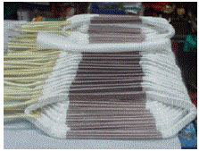
Figure 5.11. Coil sections for a 155 kVA machine; useful length: 150 mm (ECA EN document)
Let us consider the armature of the machine in Figure 5.1, with 12 slots. In a real winding, each slot has at least two independent bundles of conductors. In order to simplify the study, we shall assume that a slot has only one bundle of conductors crossed by the same current. Its commutator then has only 6 segments.
Figure 5.12 represents the corresponding lap winding, presented in a developed form. In motor operating, a direct voltage is applied to the terminals of the two brushes and generates a current I that crosses segment A of the commutator, divides into two “ways” (pairs of armature circuits in parallel) and comes back through segment D. Each conductor bundle is therefore crossed by current I/2. The adjacent conductors located in slots 1 to 6 are thus crossed by “positive” currents while slots 7 to 12 carry the return conductors crossed by “negative” currents.
Figure 5.12. Simplified lap winding, 12 slots, 2 poles, 2 “ways”, 6 commutator segments

The position of the stator poles in terms of the armature conductors is specified in Figure 5.13 for two positions of the rotor. For both positions we can notice that the current is the same in the rotor slot conductors in front of each stator pole. In the position given by Figure 5.13b, current I crosses commutator segment F and comes back via segment C. Slots 5 to 10 then contain the return conductors; the outward conductors are therefore located in the other slots.
Figure 5.13. Distribution of the armature currents for two positions of the rotor. The same current runs through the conductors in the rotor slots in front of each stator pole

If the armature keeps on rotating, current I will successively cross segments E, D, C, etc. and will respectively get out through segments B, A, F, etc., so that, in terms of the stator, the armature spatial distribution will remain unchanged. Thus the brush-commutator system makes it possible to impose on the rotor a current distribution, fixed in space and dependent on the position of the brushes. The rotor winding can therefore be modeled in a fixed axis stationary winding. This specific characteristic of DC machines will therefore be extremely useful in order to establish their equations (section 5.4.2).
We mentioned before that in practice, each slot has two conductor bundles, one taking up the top, and the other, the bottom of the slot (Figure 5.14).
An example of two-layer bipolar lap winding is given in Figure 5.15. It has 12 slots and the commutator has 12 insulated segments. In each slot, the conductor bundle corresponding to the first layer takes up the top of the slot and is represented by a continuous line. The second layer is located at the bottom of the slot and is represented by a broken line. Note that each coil section is made by the series connection of a conductor bundle taking up the top of a slot with a conductor bundle located at the bottom of another slot.
Figure 5.16 shows the field lines obtained when only the armature winding is supplied (field called “armature reaction field”). These lines turn around rotor currents; they cross the air-gap, then the stator, and then close through the rotor. In a first approximation, these lines cross only the small air-gap located under the poles.
Figure 5.17 shows the variation of the armature normal flux density along the air-gap. Origin θ = 0 corresponds to the interpolar axis. The flux density is equal to zero for θ = ±π/2 (field system poles axis), and it can be admitted that it varies in a linear way within the pole width. Around the interpolar axis, its value is small and can be assumed to be constant.
When both rotor and stator windings are supplied, the resulting field is obtained by superimposing the excitation winding and the armature fields. An example of the drawing of field lines is given by Figure 5.18. The influence of the armature reaction can be observed, which leads to a concentration of the field lines in one horn of each polar shoe.
For each pole, this phenomenon leads to the increase of the normal flux density under one horn and its decrease under the other horn (Figure 5.19). It thus leads to the magnetic saturation of the horn and of the stator teeth, subjected to the field concentration. Thus the magnetic field crossing the armature winding decreases and leads to a reduction of the electromotive force. We shall see later that this reduction can be compensated by using an extra winding at the stator, called “compensating winding” (Figure 5.47).
Figure 5.14. Armature slot having 2 conductor bundles

Figure 5.15. Lap winding, 12 slots, 2 poles, 2 layers, 2 “ways”, 12 commutator segments

Figure 5.16. Armature field lines: bipolar machine

Figure 5.17. Normal flux density in the air-gap: a) finite element calculation; b) simplified form

Figure 5.18. Distortion of the on-load field lines: bipolar machine

Figure 5.19. Normal on-load flux density: finite element calculation

5.4. DC machine equations
5.4.1. Hypotheses and covenants
We shall, in a first analysis, neglect all the losses except the Joule losses, as well as the magnetic saturation and hysteresis phenomena. The current commutation when the brushes go from one commutator segment to the next shall be assumed to be instantaneous. These various phenomena shall be the subject of a specific study at the end of the chapter.
Furthermore, since we shall assume field system current I1 and armature current I2 are perfectly constant, the field system and armature self inductances shall not take part in the equations. These parameters will have an influence only in dynamic operating or when the machines are supplied by static converters. Except if especially mentioned, we shall use the “motor” sign covenants (mechanical power considered as positive when it is supplied to a load) and, as a consequence, the two electrical circuits (armature and field system) are considered as receivers.
5.4.2. Equations
The example of simplified winding presented in Figures 5.12 and 5.13 enables us to establish a fundamental result for DC machines: the distribution of rotor currents is fixed in space and depends only on the brushes position.
The rotor coil (or the armature coil) of the machine shall therefore be likened to a fixed coil, the position of which with regard to the stator coil (or the field system coil) depends only on the brushes position. These two field systems (index 1) and armature (index 2) coils have respective self-inductances L1 and L2 and a mutual inductance M.
The DC machine has non-salient rotor poles and salient stator poles. Thus, only M and L2 depend on the respective position of the two coils, positions represented by the angle α of their respective axes (Figure 5.20). It is thus wise to derive the electromagnetic co-energy in terms of α in order to calculate the electromagnetic torque of the DC machine.
Figure 5.20. Bipolar DC machine: a) cross-section; b) schematic external representation

The general formulation of the torque (equation [2.7]) leads to:
![]()
We thus obtain:
[5.1] ![]()
Let us now consider Ohm's law applied to the rotor circuit:
![]()
where E is the electromotive force, and R2, the armature winding resistance measured between the brushes. The power absorbed by the armature is equal to:
![]()
This power is transformed, besides Joule losses ![]() , in mechanical power Pm = Γ Ω. If all the losses except for the rotor Joule losses are neglected, we have:
, in mechanical power Pm = Γ Ω. If all the losses except for the rotor Joule losses are neglected, we have:
![]()
an expression characterizing the power conservation. We obtain:
![]()
hence:
![]()
This expression shows the difference between the machine no-load electromotive force (I2 = 0), ![]() and on-load electromotive force E. However, in most cases, term
and on-load electromotive force E. However, in most cases, term ![]() can be neglected compared to
can be neglected compared to ![]() . In all the following, it shall therefore be neglected.
. In all the following, it shall therefore be neglected.
Let us now see how to choose α. Assume that only the fundamental of M(α) is taken into account (see Chapter 1):
![]()
where, in order to avoid multiplying notations, M is the maximum value of mutual inductance M(α). In this hypothesis, the expression:
![]()
leads, in modulus, to:
![]()
with the electromagnetic torque:
![]()
In order to obtain the maximum torque or the maximum emf, it is necessary to have α = π/2, that is to say M(α) = 0. The brushes are then said to be “settled on the neutral line”. In such conditions, the electrical equations of the machine are obtained:
[5.2] ![]()
[5.3] ![]()
[5.4] ![]()
These equations correspond to the schematic representation of Figure 5.21, where the field system is assumed to be supplied by a current source. The mechanical equation is written:
[2.15] ![]()
In steady state (Ω constant) Γ = ΓC. Hence in the following we shall write indiscriminately Γ or ΓC.
Figure 5.21. Conventional representation of the DC machine

5.4.3. Determination of the parameters
Equations [5.2] to [5.4] enable us to study the steady state of DC machines, providing their supply and implementation modes are known: separate excitation machine or series excitation machine. In order to predetermine the working of a particular machine, it is therefore necessary to determine parameters R2, R1 and M.
5.4.3.1. Resistance measurement
The measurement of R1, static coil resistance, is not particularly a problem. A standard “ammeter-voltmeter” method enables us to determine its value with satisfying precision. Alternately, the determination of R2 is more difficult.
Let us consider Figures 5.13 and 5.15. The current goes from one brush to another by circulating through a number of conductors connected in series and in parallel. When the rotor turns, this conductor repartition is modified because the brushes are successively in contact with one or several commutator segments. The result is that the value of resistance R2 depends on the rotor position. Furthermore, at the brush-commutator contact, there is a voltage drop Δu depending on the contact surfaces, on the pressure and on the value of the current.
R2 therefore appears to be a very simple model for the representation of complex phenomena; strictly speaking, its dependency upon Θ and I2 should be taken into account. In order to take into account the dependence on R2 in relation to Θ, it is advisable to make measurements with various rotor positions and to take the average. For the dependence on I2, it is advisable to repeat the previous measurement for various values of the armature current and to tabulate the obtained results. For simplicity's sake, this determination is generally only achieved with the nominal current and under the normal operating temperature. This induces an acceptable lack of precision.
5.4.3.2. Measurement of M
Expression [5.3] shows that if E, Ω and I1 are known, it can be deduced:
[5.5] ![]()
For this, a “no-load generator” test is achieved: the studied machine is driven by an auxiliary motor (Figure 5.22), a current I1 is injected in the excitation circuit and voltage U = E is measured at the armature terminals, in which no current circulates. So that mutual M may be considered to be constant, it is advisable to restrict the value of I1 (I1 < I1l) in order to avoid magnetic saturation (Figure 5.23).
Figure 5.22. No-load generator test

Figure 5.23. Independent excitation no-load generator characteristic

5.5. Separately excited motor
5.5.1. Introduction
This is the most common use of the DC motor. The field system and the armature are supplied separately by two supposedly distinct sources, which allows us to separately impose field system current I1 and voltage U to the armature terminals.
We shall now analyze how the various variables appearing in equations [5.2] to [5.4] vary according to the different operating modes of the machine. A “system” approach of the machine highlights (Figure 5.24) two “inputs” U and I1 (supposedly controllable values), a “perturbation” Γ = Γc imposed by the environment (Γc is the load resistant torque that the motor has to drive) and two “outputs” Ω and I2, values for which evolutions in terms of the inputs and of the perturbation are determined by the machine equations.
The characteristics are therefore the curves representative of the output variations in terms of one of the three other values, the other two supposedly being constant. It is therefore advisable to formulate the two output expressions in terms of the inputs and of the perturbation.
Figure 5.24. “System” representation of the separately excited motor

We therefore have:
[5.6] ![]()
and:
[5.7] ![]()
Those two expressions make it possible to draw the separately excited machine characteristics. In the following paragraphs we shall determine these characteristics by considering a “model machine” for which the parameters are the following:
– nominal power: Pn = 4 kW;
– nominal armature voltage: U = 220 V;
– nominal armature current: I2n = 22 A;
– nominal field system current in motor operating: I1n = 1.1 A;
– nominal field system current in generator operating: I1n = 1.6 A;
– armature resistance: R2 = 0.5 Ω;
– field system resistance: R1 = 133 Ω;
– mutual inductance: M = 1.27 H;
– nominal speed: Ωn = 157 rd/s.
5.5.2. External characteristics
5.5.2.1. Characteristic I2 = f(Γ) with constant U and I1
Equation [5.6] corresponds to a straight line going through the origin and to slope 1/(MI1) (Figure 5.25).
Figure 5.25. Characteristic I2 (Γ) with constant armature voltage and field current

5.5.2.2. Characteristic Ω = f(Γ) with constant U and I1
The motor speed is given by expression [5.7]. Note that, as U and I1 are fixed, Ω varies linearly in terms of Γ (Figure 5.26). It is a straight line of origin ![]() and of slope
and of slope ![]() . This straight line with a small slope, and we deduce that the rotation speed of a separately excited motor is almost independent of the load torque value.
. This straight line with a small slope, and we deduce that the rotation speed of a separately excited motor is almost independent of the load torque value.
Figure 5.26. Characteristic Ω(Γ) with constant armature voltage and field current

5.5.2.3. Characteristic Ω = f(U) with fixed Γ and I1
This is an important characteristic for separately excited DC motors. Equation [5.7] represents a straight line of slope 1/(MI1) which starting abscissa depends on Γ (Figure 5.27). As the term ![]() is usually small, we deduce that in a first approximation, the rotation speed of this kind of motor is proportional to the armature voltage.
is usually small, we deduce that in a first approximation, the rotation speed of this kind of motor is proportional to the armature voltage.
Figure 5.27. Characteristic Ω (U) with constant torque and field current

This property is largely used for industrial variable speed drives, where separate excitation motors are supplied by static converters.
5.5.2.4. Characteristic I2 = f(U) with fixed Γ and I1
With Ω = 0, we can be write:
![]()
It is therefore necessary to have ![]() for the motor to start. Below this value, the armature behaves as a resistance, and therefore I2 = U/R2. Above this limit, I2 = Γ/(MI1) is constant (Figure 5.28).
for the motor to start. Below this value, the armature behaves as a resistance, and therefore I2 = U/R2. Above this limit, I2 = Γ/(MI1) is constant (Figure 5.28).
5.5.2.5. Characteristic I2 = f(I1) with fixed Γ and U
If Γ is fixed, equation [4.6] shows that current I2 hyperbolically varies in terms of I1 (Figure 5.29). If I1 tends toward zero, I2 therefore tends toward infinity, and it can thus be dangerous to reduce the field system current too much.
Figure 5.28. Characteristic I2(U) with constant torque and field current
Figure 5.29. Characteristic I2(I1) with constant armature voltage and torque

5.5.2.6. Characteristic Ω = f(I1) with fixed rand U
Equation [4.7] shows that, in order to obtain Ω > 0, it is necessary to have ![]() . It is also clear that if I1 tends toward infinity, the rotation speed Ω, tends toward zero. Furthermore, note that if I1 tends toward zero, Ω tends toward –∞. This result, which corresponds to the curves of Figure 5.30, has to be considered with caution. Indeed when these curves are considered, note that when I1 decreases, speed goes through a maximum (
. It is also clear that if I1 tends toward infinity, the rotation speed Ω, tends toward zero. Furthermore, note that if I1 tends toward zero, Ω tends toward –∞. This result, which corresponds to the curves of Figure 5.30, has to be considered with caution. Indeed when these curves are considered, note that when I1 decreases, speed goes through a maximum (![]() with
with ![]() .
.
Figure 5.30. Characteristic Ω(I1) with constant voltage and torque

This theoretical maximum is much higher than the actual speed the machine can tolerate, hence the usual expression: “if the field system current is lowered too much, the machine races”. If current I1 is accidentally switched off, the machine behavior will depend on the load. If the motor does not have any mechanical load, it will have a tendency to race (Ω → ∞ if I1 → 0, with Γ = 0). On the contrary, if the load torque exists, mechanical equation [2.15] shows that the speed is cancelled when Γ is zero; the machine will then “stall” and there is a risk of damage due to an excessive armature current. It is obvious that it is very important to avoid any accidental switching off of the field system current.
All of these characteristics show that the separately excited DC machine gives a very interesting possibility for the design of variable speed drives. It is indeed very convenient to control it with the armature voltage, the great simplicity of the equations linking U to Ω and to I2 allowing the use of very simple speed and current controllers.
The influence of I1 on the speed variation is more complex and hazardous. In practice, the adjustment of Ω by I1 is only used to obtain a speed increase beyond the maximum value of U. I1 is then decreased to accelerate the motor. It is important to note that this can only be done if the torque is smaller than the nominal torque (see equation [5.4]).
5.5.3. Energy recovery: generator operating
In the past, separately excited machines were used to produce direct current. This working mode has almost disappeared with the rise of static rectifiers. This machine however enables it to recover kinetic energy during braking or slowing down, within the devices where they mostly play the part of motors.
Figure 5.31 schematizes the generator working of the separately excited machine. In this case, it is judicious to modify the sign covenant for the armature, which shall be considered as a generator.
If the “system” analysis is used again, note (Figure 5.32) that, in this case, I1 and U remain inputs, and I2, an output.
Rotation speed Ω is usually imposed by the mechanical environment and has to be considered as a perturbation. Conversely, torque Γ = M I1 I2 is an output.
By adopting the “generator” sign covenants (electrical power considered as positive when it is supplied to a load), equations [5.2] to [5.4] become:
[5.2'] ![]()

The output expressions become:
[5.8] ![]()
[5.9] ![]()
Figure 5.31. Conventional representation for generator mode

Figure 5.32. System inputs and outputs

In the following we shall outline the characteristics by referring to the “model” machine defined in section 5.5.1.
5.5.3.1. Operating mode with fixed U and Ω
Equations [5.8] and [5.9] highlight a minimum value of field system current I1 = U/(MΩ) enabling the energy recovery. Characteristic I2 = f(I1) is a straight line starting from this minimum value and of slope MΩ/R2 (Figure 5.33). The torque variation in terms of I1 is a parabola (Figure 5.34).
Figure 5.33. Characteristic I2(I1) with constant voltage and speed
Figure 5.34. Characteristic Γ(I1) with constant voltage and speed. Note that the useful part of the parabola is almost linear

5.5.3.2. Variable voltage operating
Characteristics I2(U) and Γ(U) are straight lines that cut the axes in points U = MΩI1 and respectively ![]() and
and ![]() (Figures 5.35 and 5.36).
(Figures 5.35 and 5.36).
Figure 5.35. Characteristic I2(U) with constant excitation and speed. Point (U = 0, I2 = MΩI1/R2) is out of the frame of the figure

Figure 5.36. Characteristic Γ (U) with constant excitation and speed. Point(U = 0, Γ = (MI1)2Ω//R2) is out of the frame of the figure
5.6. Series excited motor
5.6.1. Introduction
In a “series excited” DC motor, or “series motor”, the field system and the armature are connected in series and supplied by the same continuous voltage source. This brings a constraint on the field system which, as it is travelled by the armature current, has to have a small enough resistance to prevent a reduction of the global efficiency. The field coil is therefore made of quite a small number of turns of important section conductors. Note that this increases the machine inductance, which is favorable when it is supplied by power converters.
Figure 5.37 shows the conventional representation of the machine. In this case, the machine equations become:

In order to simplify, we set down R = R1 + R2.
Figure 5.37. Conventional representation of the series excited machine
This system has one degree of freedom less than the separately excited motor; the supply voltage U is now the only “input” (Figure 5.38).
Figure 5.38. “System” representation of the series excited machine

The characteristics of this motor are therefore the variation curves of Ω and I in terms of U or to Γ, the other value remaining constant. Let us then write the expressions of I and Ω:
[5.10] ![]()
[5.11] ![]()
5.6.2. External characteristics
In order to outline the characteristics of series motors we shall use the parameters of the following “model” machine:
– nominal power: Pn = 4 kW;
– nominal armature voltage: U = 220 V;
– nominal current: In = 22 A;
– armature resistance: R2 = 0.5 Ω.
– field coil resistance: R1 = 0.375 Ω;
– mutual inductance: M = 58.1 mH;
– nominal speed: Ωn = 157 rd/s.
5.6.2.1. Characteristic I(Γ) with U = constant
Current I is given by [5.10], its variation in terms of Γ is represented by Figure 5.39. It is a parabola going through the origin.
Figure 5.39. Characteristic I(Γ) with constant voltage, U = UN

5.6.2.2. Characteristic Ω = f(Γ) with fixed U
The expression of speed is given by equation [5.11]. If U is assumed to be constant, and Γ variable, we obtain a curve with hyperbolic appearance (Figure 5.40) emphasizing that if Γ tends toward 0, the motor races (speed tends toward infinity). This is a fundamental feature of the series motor, for which no-load operation is not allowed in order to prevent it from racing.
Figure 5.40. Characteristic Ω(Γ) with constant voltages, U = UN and UN/2

It is however noted that speed has an important variation in terms of the load torque. Theoretically Ω would be zero when Γ = M (U/R)2; this very important value corresponds to a current I = U/R much greater than the nominal current. This however characterizes the ability of the series motor to provide a very important starting torque.
5.6.2.3. Characteristic Ω = f(U) with constant Γ
This characteristic (Figure 5.41) is a straight line going through the point with the coordinates Ω = 0 and ![]() . Note that the motor only starts for a voltage higher than
. Note that the motor only starts for a voltage higher than ![]() .
.
Figure 5.41. Characteristic Ω (U ) with constant torque, Γ = ΓN and ΓN/2

5.6.2.4. Characteristic I = f(U) with constant Γ
Current I given by equation [5.10] is constant when the motor works, that is to say for ![]() . Below this value, the motor behaves like a resistance R and the current is worth I = U/R (Figure 5.42).
. Below this value, the motor behaves like a resistance R and the current is worth I = U/R (Figure 5.42).
Figure 5.42. Characteristic I(U) with a constant torque, Γ = ΓN and ΓN/2

5.7. Special case of the series motor: the universal motor
A universal motor is a series machine capable of being supplied in direct current as well as in alternative current. We have indeed seen that the series machine torque is proportional to the square current; it is therefore independent from the direction of the current circulation and can thus be supplied with alternative current.
However, comparative to the standard series motor, this kind of motor has to have a laminated stator in order to minimize the iron losses (see Chapter 2). The number of turns in the field winding has to be reduced in order to restrict the stator inductance. In order to compensate for the reduction of the excitation flux, the rotor turns number increases accordingly.
As with all series motors, the universal motor races at no-load and its speed is very dependent on its load. It is used in devices requiring a good starting torque: traction, domestic appliances, etc.
5.8. Commutation phenomena
The commutation phenomenon appears when a brush goes from one commutator segment to the next because the current has to reverse in one coil section. The latter being inductive and submitted to induced electromotive forces, the reversal of the current is not instantaneous. We shall restrict the study to the case of “simple” commutation, that is to say when the brush width is equal to the commutator segment width.
Let us consider the example given in Figure 5.43, representing an armature with 12 slots, 12 commutator segments, 2 poles and 2 conductor layers. In Figure 5.43a, each brush covers a single commutator segment. At this instant, the current in the coil section made of conductors 1 and 7 is considered to be positive and worth I/2.
Figure 5.43. Transition of the brushes from a commutator segment to the next: a) brush in contact with a single segment; b) brush short-circuiting two segments

In Figure 5.43b, which shows a later instant, the brushes, overlapping two segments, short-circuit two coil sections. A still later instant, when the brushes leave left segments A and G of the commutator to position themselves on segments B and H, the current in coil section 1–7 changes its sign and goes from I/2 to –I/2.
If the armature diagram is simplified (Figure 5.44), it is noticed that when the brush overlaps 2 commutator segments, the corresponding coil section (noted “S” on the figure) is short-circuited. Current Is in this coil section will therefore vary according to the flux that crosses it and to its impedance.
Depending on the cases, the variation of Is (from I/2 to – I/2) can have various aspects (Figure 5.45):
– on curve (1), Is varies linearly, which corresponds to a current density constant on brush-commutator contact. This constitutes the ideal commutation;
– on curve (2), the current does not vary linearly, but naturally reaches -I/2 when the brush leaves commutator segment A;
– for curves (3) and (4), the current does not reach -I/2 when the brush leaves commutator segment A. There is therefore a current discontinuity on brush-commutator contact, which has to go instantly from (IS + I/2) to zero. This current discontinuity generates an arc at the moment when the brush leaves the commutator segment. If this discontinuity is important, the arc can damage the commutator and the brushes. In any case, these arcs are ageing factors that are prejudicial to the brush-commutator set life duration.
Without going into detail, it is advisable to point out at this stage that the commutation phenomena are even more complex when the armature current is alternative (universal motors) or, to a lesser extent, have an important harmonic content (case of static converter supply).
In order to improve the commutation, the flux in the short-circuited section has to be reduced. This can be obtained either by shifting the brushes (for small power motors), or by using an extra winding called “commutation winding”. This commutation winding is set down between the main poles and supplied with the armature current (Figures 5.46 and 5.47).
Figure 5.44. Schematic representation of the moving of a brush from one segment to the next

Figure 5.45. Evolution of the current in a coil section in commutation. On t1, the brush comes into contact with the second commutator segment B, and on t3, it leaves initial segment A

Figure 5.46. Main poles and commutation poles of a bipolar machine

5.9. Saturation and armature reaction
As for all electromechanical converters, DC machines are subjected to the magnetic saturation phenomenon. This leads to a non-linear no-load characteristic E = f(I1) (Figure 5.23). This phenomenon is amplified by the armature reaction effect. Indeed, we have seen in paragraph 5.3.3, by considering Figure 5.18, that the field lines concentrate in one of the polar horns to the detriment of the other horns. This leads to a local saturation and to the reduction of the useful flux.
Figure 5.47. Stator of a four-pole machine, 220 kW, 440 V, 2,800 to 7,000 rpm. The field system windings, commutation windings and compensation windings can be distinguished (ECA EN document)

To overcome this problem, a winding called “compensation winding” is used. It is located in slots gouged into the stator pole pieces and supplied with the armature current. This leads to the stator structure represented in Figure 5.47, where the field winding, the commutation winding and the compensation winding are visible.
5.10. Implementation of DC motors
Nowadays it is necessary to distinguish, on the one hand, the traditional implementation with constant voltages (it has a historical and a pedagogical interest), and on the other hand, the present implementation using static converters.
5.10.1. Constant voltage implementation
When a DC machine, either a separate or series excited machine, is supplied with constant voltage, the main difficulty is to ensure it starts. Indeed, when at standstill, the machine has no electromotive force and the absorbed current is limited only by small value resistances (R2 in the case of separate excitation or R1 + R2 in the case of series excitation). The aim is therefore to restrict the absorbed current to a value acceptable for the machine, while maintaining a torque sufficient for the start. Since the thermal time constants are noticeably greater than the mechanical time constants, it is acceptable to have, during transient states, and in particular during starting, a current greater than the nominal current. If the starting current is called Id we have:
![]()
“Over-current” coefficient k is usually around 2.
5.10.1.1. Separately excited motor start
In order to study the start, we shall admit that the armature electrical time constants can be overlooked compared to the mechanical time constants. This will enable us to assume that the armature current variations are instantaneous.
Let us consider a machine supplied with its armature nominal voltage and with its nominal field current. It is mechanically connected to a load for which the resistant torque Γc is equal to the motor nominal torque. In order to reduce the current absorbed during the start, a “starting rheostat” Rd is inserted between the source and the motor armature (Figure 5.48)
Figure 5.48. Rheostatic starting

By calling Rd0 the value of Rd necessary for current I2 to be equal to kIn at standstill we get:
![]()
thus:
![]()
At the switching on of the armature, motor torque Γ will therefore be equal to k M I1n I 2n, which leads to the equation:
![]()
The machine will therefore start and will generate an electromotive force MΩI1n with:
![]()
thus:
![]()
The armature current will therefore decrease with the machine acceleration. The motor torque given by:
![]()
is therefore variable in terms of the rotation speed. The equation of the dynamic:
![]()
shows that the motor accelerates until Γ = Γc, value obtained for I2 = I2n. The corresponding rotation speed Ω1 is:
![]()
The value of the starting resistance can then be modified to a value Rd1 defined by:
![]()
The motor will accelerate again to:
![]()
The process is then iterated until complete cancellation of the starting resistance.
Figure 5.49 represents the time variations of the armature current and of the speed of the “model machine” presented in section 5.5.1 during a nominal torque start.
Figure 5.49. Starting of the separately excited motor (example motor): a) armature current variation b) speed variation

5.10.1.2. Particular case of the separately excited motor: DC shunt motor
When there is only one voltage source, the armature and the field system are connected in parallel to this source, the armature through the starting resistance, and the field system through another rheostat called a “field rheostat” and noted Rh in Figure 5.50.
Figure 5.50. Shunt motor implementation

During starting, Rh is usually short-circuited in order to have maximum I1 and the greatest possible torque. Voltage source U is applied to the cursor of the starting rheostat so that, when Rd is short-circuited, its resistance adds to the resistance of the field system. Current I1 decreases and reaches I1 = I1n at the end of the starting. Rh then enables us to make I1 decrease in order to increase speed Ω.
5.10.1.3. Series motor starting
A starting rheostat is also used to reduce the current to kIn and the iterative process leading to the progressive removal of Rd is identical. The only notable difference is that Γ is proportional to the square of I, the starting torque is multiplied by k2 which gives, for the series motor, a great starting torque.
5.10.2. Present implementation of DC motors
5.10.2.1. Separately excited motor
Figure 5.51 represents a separately excited motor for which the armature is supplied by a 3-phase thyristor bridge. The control variable Vc of the pulse generators (not represented in order to avoid complicating the figure) is the output of a current and speed controller. This controller receives on the one hand current reference (Ref I) and speed reference (Ref Ω), and on the other hand the signals given by the corresponding sensors. The current reference usually corresponds to the maximum value acceptable by the motor: Ref I = kI2.
Figure 5.51. Separately excited motor implementation

Without going into the details of the control, a fast internal loop is used to control the current and prevent it from being greater than the fixed limit during transients and particularly during starting.
Since, in a first approximation, output voltage U of the thyristor bridge is proportional to Vc, and rotation speed Ω is also proportional to U, the speed controller of the motor is simple to implement. If we want the motor to turn in both directions (reversibility in Ω and in Γ, a two-bridge “back to back” structure is used, as represented in Figure 1.26.
5.10.2.2. Series motor implementation
Figure 5.52 represents a series motor supplied by a step-down chopper. The fully controllable switch Tc (it can be turned on and off at will) is a power transistor, an IGBT, even a GTO for very high powers.
The variation of the duty cycle α (see Chapter 1) makes it possible to impose the average value of voltage U applied to the motor (U = αU0), and therefore its average speed in steady state. The control has two loops: an internal “fast” loop for current control enabling us to limit I under kIn in dynamic operating mode, and a slower external loop for speed control. In order to recover the kinetic energy during slowing down and motor braking, it is necessary to use a reversible chopper (see section 1.3.3).
Figure 5.52. Implementation of a series motor supplied by a chopper
