Chapter 4
Induction Machines
4.1. Introduction
“Induction machines” are energy converters characterized by the fact that the rotation speed of their rotor is different from the synchronous speed, defined by:
![]()
where ω is the angular frequency of the stator currents, and p is the number of pole pairs. These machines are called “induction machines” because their rotor currents are generally induced by the currents running through the stator coils.
These machines are rustic, robust and cheap. Formerly their use was restricted to simple and low performance applications when they were connected to constant frequency and constant voltage networks.
Now, induction machines have spread in every domain of industrial motorization, including high-tech applications, since the recent progress in power electronics and in digital control have made it possible to control them with good dynamic performance.
4.2. General considerations
4.2.1. Structures
4.2.1.1. Stator
The stator of induction machines is a 3-phase field spool with 2p non-salient poles identical to the stator of synchronous machines (Figure 4.1). It is connected, either with a 3-phase network, or with a static converter, and a 3-phase current system is produced.
Figure 4.1. Induction machine stator before winding, 45 kW, 440 V, 590 rpm (ECA EN document)

4.2.1.2. Rotors
Two types of rotors exist: rotors called “wound rotors” and rotors called “squirrel rotors”.
4.2.1.2.1. Wound rotors
In this case, we have a 3-phase field spool with 2p non-salient poles, star connected, in which each phase is connected to a slip-ring on which a fixed brush is rubbing (Figure 4.2). This device makes it possible to connect the rotor coil to either a starting 3-phase rheostat, or to a static converter for some particular drives. In usual working, the 3-phases are short-circuited and 3-phase currents are induced by stator currents. This configuration is mainly found in high-power machines.
Figure 4.2. Wound rotor of induction machine, 140 kW, 380 V, 800 rpm, shaft height: 355 mm (ECA EN document)

4.2.1.2.2. Squirrel rotors
In this case, the rotor is hollowed out of longitudinal slots in which conductive bars are placed and short-circuited at each end by “short-circuit rings” (Figures 4.3 to 4.6). Those bars and rings are usually made of copper but, for small power machines, they can be made of aluminum alloy in order to reduce the cost price. This structure is not a 3-phase structure, but for each cage rotor, an equivalent 3-phase wound rotor can be determined.
As the external behavior of the two types of machines is similar, we shall consider, in this chapter, that we are dealing with wound-rotor machines for which equations are easier to set.
4.2.1.3. Air-gaps
In the two cases (wound rotor and squirrel rotor), it is possible to consider, in an initial approximation, that the air-gap is constant.
We shall see in the following that the induction machine performances are very dependent on the thickness of this air-gap, which is, as a consequence, as small as possible: it varies from a few tenths of a millimeter for the small power machines to a few millimeters for the high power machines.
Figure 4.3. Squirrel rotor of induction machine, 6 kVA, 440 V, 60 Hz, 1 200 rpm. Note the skew of the slots (ECA EN document)

Figure 4.4. Piling up of steel sheets constituting the magnetic circuit of a squirrel rotor (photo source: Converteam)

Figure 4.5. Detail view of a squirrel rotor being built. Note the cooling holes (photo source: Converteam)
Figure 4.6. Squirrel rotor. The short-circuit ring connecting the bars to one another is visible as well as the fan on the shaft (photo source: Converteam)
4.2.2. Working principle
Let us assume that the stator windings fed by 3-phase currents of angular frequency ω will correspond to an air-gap field rotating at angular speed:
![]()
where Ω is the rotor speed. If Ω ≠ Ωs the flux in the rotor phases are time variable and give rise to electromotive forces. Since the rotor phases are short-circuited, these electromotive forces generate currents, which, through an interaction with the stator field, give rise to a torque. On the contrary, if Ω = Ωs, the rotor flux do not depend on time, and there are therefore neither electromotive force nor induced currents at the rotor. It is therefore clear that, with such machines, the energy conversion requires that the speeds of the rotor and of the air-gap field are different; that is the reason why they are also called “asynchronous machines”. The relative difference in speed between the field and the rotor, or “slip”, plays an important part in the study of induction machines. Slip g is defined by:
![]()
thus ![]() .
.
Θ measures the position of the rotor with regard to the stator. When introducing electrical angle θ, we write:
![]()
4.3. Equations
In this section, we are going to establish the external behavioral equations of the induction machines using the coupling matrixes of the stator and rotor phases.
4.3.1. Main notations
If the machines are assumed to be 3-phase at the rotor as well as at the stator, and the axis of phase A is chosen as the origin of the angles, we shall call:
– A, B, C: stator phases;
– a, b, c: rotor phases;
– g: slip;
– Is: rms stator current value;
– Ir: rotor currents efficient value;
– J: moment of inertia;
– Li: phase i self inductance;
– Mij: mutual inductance between phases i and j;
– M0: maximum value of the mutual inductance between a stator phase and a rotor phase;
– p: number of stator and rotor pole pairs;
– Θ : stator-rotor mechanical angle;
– θ = pΘ: electrical angle;
– ω : stator currents angular frequency;
– ωr: rotor currents angular frequency;
– Ω = dΘ/dt: rotor speed;
– Ωs = ω/p: synchronous speed;
– {is}: stator currents vector;
– {ir}: rotor currents vector;
– {Ls}: stator inductance matrix;
– {Lr}: rotor inductance matrix;
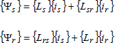
– {Lsr} = {L rs}t: stator-rotor coupling matrix;
– {Ψs}: vector of the total flux per stator phase;
– {Ψr}: vector of the total flux per rotor phase.
4.3.2. Sign covenants and working assumptions
Throughout this chapter, we shall adopt the “motor” sign covenants for the machine, which means that the mechanical power will be considered as positive if it is produced, and the electrical power will be positive if it is absorbed. We shall therefore take, a priori, “receiver” sign covenants for each of the electrical circuits.
The coils are assumed to have a sinusoidal ampere-turns distribution, and we shall neglect the saturation and hysteresis phenomena.
4.3.3. Conventional representation
Figure 4.7 represents in a conventional way the stator and rotor windings.
Figure 4.7. Conventional representation of the machine

4.3.4. Flux analysis
If the matricial general expression is considered again:
[4.1] ![]()
or:
[4.2] ![]()
with:
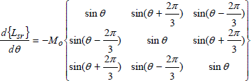
the machine has non-salient poles both at the stator and at the rotor, only the stator-rotor coupling inductances depend on the position, and we can write;

where Ls and Ms are the self and mutual inductances of the stator phases, and Lr and Mr are the self and mutual inductances of the rotor phases. In the same way, we have:

Furthermore, we can write the stator and rotor currents in the vectorial form:

φs and φr are respectively the stator and rotor currents phases corresponding to the voltages taken as the phase origin. It is therefore possible to express the total flux per stator and rotor phase:
To simplify the calculations, we shall develop only the first line of these two equations for the determination of ΨA and Ψa:

with θ = θo + (1-g)ωt.
If the currents are replaced by their expressions in terms of time, we get:
[4.3] ![]()
In the same way, we obtain:
[4.4] ![]()
Expressions [4.3] and [4.4] show that the total flux per stator and rotor phase are sinusoidal values of respective angular frequencies ω and gω. It is therefore possible to use the complex notations associated with these sinusoidal values.
Given ![]() A,
A, ![]() a, ĪA and Īa the complex representations respectively associated with ΨA, Ψa, iA and ia; equations [4.3] and [4.4] lead to:
a, ĪA and Īa the complex representations respectively associated with ΨA, Ψa, iA and ia; equations [4.3] and [4.4] lead to:
[4.5] ![]()
[4.6] ![]()
NOTE.– Since complex formalism makes angular frequencies disappear, we shall note them down separately in order to avoid any possible ambiguity.
It is obvious that, in the other stator and rotor phases, we would obtain similar expressions. It is therefore possible to unify the expression of the total flux per stator and rotor phase in making the following variable changes:
– ĪA ⇒Ī1: stator current or “primary current”;
– ![]() : “secondary” current;
: “secondary” current;
– ![]() “primary” flux;
“primary” flux;
– ![]() : “secondary” flux.
: “secondary” flux.
In setting down:
– L1= LS – MS: primary synchronous inductance;
– L2 = Lr – Mr: secondary synchronous inductance;
– M = 3/ 2M0;
– R1 = Rs;
– r2 = Rr;
equations [4.5] and [4.6] become:
[4.7] ![]()
[4.8] ![]()
4.3.5. Electrical equations
If the induction machine has its rotor short-circuited and its stator supplied by a balanced 3-phase voltage system of rms value per phase V1, it can be written:

that is to say:

From the two equations [4.7] and [4.8], we get:
[4.9] ![]()
[4.10] ![]()
These two equations can be written under the matrix form:
[4.11] 
4.3.6. Change in the sign covenant
Equation [4.11] is very similar to the equation of a single-phase transformer, without iron losses or secondary resistance, loaded on a resistance R2/g. In order to make use of this similarity, it is natural to alter the sign covenant for the secondary current (rotor) and to choose, for induction machines rotors, the “generator” sign covenant (output current counted positively). It can be noted that, since the rotor windings are in short-circuit, this alteration has no energy consequences. In such conditions, equation [4.11] becomes:
[4.12] 
4.4. Equivalent circuits
Equation [4.12] corresponds to an equivalent circuit per phase, identical to that of a single-phase transformer with stator Joule losses only (Figure 4.8).
Figure 4.8. Induction machine equivalent circuit

The transformer appearing on this equivalent circuit has a voltage ratio ![]() . The dispersion coefficient is also introduced:
. The dispersion coefficient is also introduced:
![]()
This diagram enables us to represent the energy flux in the machine. Term 3R1I12 represents the Joule effect losses at the stator and ![]() corresponds to the overall power transmitted to the rotor. In order to separate the converted power from the rotor Joule losses, it is necessary to slightly modify the equations and the equivalent diagram of the machine. We shall therefore write:
corresponds to the overall power transmitted to the rotor. In order to separate the converted power from the rotor Joule losses, it is necessary to slightly modify the equations and the equivalent diagram of the machine. We shall therefore write:
[4.13] 
which leads to the equivalent circuit given in Figure 4.9.
Figure 4.9. Equivalent circuit separating the Joule losses from the converted power

On the one hand, this diagram clearly shows the rotor Joule losses ![]() appear and, on the other hand, the converted power
appear and, on the other hand, the converted power ![]()
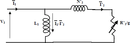
In the following we shall see that it is sometimes convenient to use a transformer-less equivalent diagram based on a two-terminal network. We shall therefore set down:
– ![]() rotor current referred to the stator;
rotor current referred to the stator;
– ![]() : resistance of a rotor phase referred to the stator;
: resistance of a rotor phase referred to the stator;
![]() with
with ![]() : total leakage inductance seen from the rotor.
: total leakage inductance seen from the rotor.
In transferring these variable changes in equations [4.9] and [4.10] we finally have:
[4.14] ![]()
[4.15] ![]()
These two equations correspond to the equivalent diagrams of Figures 4.10. Figure 4.10b separates the rotor Joule losses from the converted power.
Figure 4.10. Transformerless equivalent circuits

4.5. Induction machine torque
4.5.1. Instantaneous torque
The expression of the induction machine instantaneous torque can be established from general expression [2.8a]:
![]()
The stator and rotor currents are assumed to be sinusoidal, in a balanced 3-phase system, with respective angular frequencies ω and gω, we shall set down:

with:
and:
![]()
We finally get:
[4.16] ![]()
This expression shows that in sinusoidal steady state, the induction machine instantaneous torque is constant. It will therefore be possible to identify this instantaneous torque with the average torque determined from global energy considerations.
Expression [4.16] is not convenient to use because it depends on values that are difficult to obtain, such as θo and φr; we shall therefore establish another torque formulation from the analysis of the energy transfer in the induction machine.
4.5.2. Analysis of the energy transfer
Let us assume that the machine is connected to a network having a phase voltage V1. The absorbed active power is written Pa. The latter is partially dissipated in stator Joule losses pj1 and of stator iron losses pf1 (which had until now been neglected). The remaining power, which shall be called P2, is transmitted to the rotor:
[4.17] ![]()
Referring to the equivalent diagram of Figure 4.8, it can also be written:
![]()
In the rotor, the frequency is small (ωr = gω), and it is therefore possible to neglect the rotor iron losses. After taking off the rotor Joule losses pj2, P2 is converted into mechanical power Pm = ΓΩ.
Considering the equivalent diagram given in Figure 4.9, we get:
![]()
![]()
hence:
![]()
and therefore:
[4.18] ![]()
This result shows that the power transmitted to the rotor is equal to the product of the torque by the synchronous speed. Furthermore, since pj2 = gP2, it is clear that the rotor Joule losses are proportional to the slip, and therefore inherent to the asynchronous energy conversion. This power transfer can be represented by Figure 4.11.
Figure 4.11. Power transfer in the induction machine

It is also deduced that if all losses except pj2 losses were neglected, the ideal efficiency would at the most be equal to:
![]()
This expression shows that in order to have a satisfying efficiency, an induction machine has to work with a small slip.
4.5.3. Expression of the electromagnetic torque in terms of the slip
For this study, we shall neglect all the stator losses. The equivalent circuit per phase of Figure 4.10a becomes that of Figure 4.12.
Figure 4.12. Equivalent figure without stator losses
The value of P2 can be deduced from this diagram:
![]()
We therefore have ![]() , with:
, with:

thus:
[4.19] 
Expression [4.19] makes it possible to study the variation of the torque of the induction machine in terms of the slip (Figure 4.13). This characteristic curve, drawn for a slip varying from –∞ to +∞, leads to the following remarks:
– if g is near zero,![]() leads to
leads to ![]() .
.
We can deduce that curve Γ(g) is almost linear when nearing the origin;
– if g is important,![]() leads to
leads to ![]() The torque will therefore hyperbolically tend toward zero if g tends toward infinity;
The torque will therefore hyperbolically tend toward zero if g tends toward infinity;
- curve Γ(g) has two extreme values ![]() obtained for:
obtained for:
![]()
It is therefore clear that obtaining an important value of Γm will be linked to a small value of N'2 corresponding to small stator-rotor leakage. This explains that induction machines have as small an air-gap as possible.
Figure 4.13. Torque-slip characteristic

Curve Γ(g) is symmetrical in relation to the origin. It is therefore clear that if g is negative (Ω > Ωs), the electromagnetic torque is negative too, which characterizes a negative mechanical power. This shows the reversibility of the induction machine, which can operate as a generator or as a motor.
4.6. Study of the stability
Let us assume that the machine, working as a motor, drives a charge characterized by a resistant torque ΓC (Figure 4.14). We observe that characteristics Γ(g) and ΓC(g) have two intersections for working points corresponding to slips called gC and gC'. In order to show that only slip point gc corresponds to an effective working point, we shall study the induction machine stability.
Figure 4.14. Stable parts of the torque-slip characteristic

Let us assume that the machine is in steady state with slip gC and that a perturbation Δg occurs. If Δg is small enough, the characteristics Γ(g) and ΓC(g) can be assimilated with their tangential lines in gc :

and:
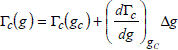
Furthermore:
![]()
hence:
![]()
The mechanical equation therefore becomes:
![]()
Remember that in this equation, J represents the moment of inertia of all the rotating parts (rotor of the induction machine and load).
In order for the calculation to be stable, the machine must tend to get back to its initial working point, that is to say that g tends toward gc and therefore that ![]() and Δg have opposite signs. It is then necessary to have:
and Δg have opposite signs. It is then necessary to have:
[4.20] 
Generally the resistant torque increases with speed, consequently it decreases with slip. The condition for stability [4.20] can therefore be written:
[4.21] ![]()
We can deduce that the stable part of characteristic r(g) is the part located between g = -gm and g = +gm, in the small slip area. In Figure 4.14, the stable operating point corresponds to g = gc. The point corresponding to g'C is therefore unstable.
4.7. Circle diagram (or “Blondel” diagram)
4.7.1. Introduction
From its origins, electrical engineering has used graphic methods for the predetermination of the behavior of the machines, particularly that of AC machines. Indeed the latter are governed by equations that are difficult to treat in an analytical way.
Since digital calculation has been developed, diagrams have lost the part of “calculation instruments” that they had played for decades, to become mere support for qualitative reasoning, and for digital calculations that avoid the structural imprecision of the graphic methods.
This is true both for induction machines and for synchronous machines. That is why, in this book, we shall mainly use the simplified version of the circle diagram, called a “Blondel diagram”. This diagram represents, in the complex plane, the locus of the vector of affix Ī1 when slip g ∞ to + ∞, with constant V1 and ω. If matrix equation [4.13] is considered again and if current Ī2 is eliminated, we have:
[4.22] 
The stator phase impedance ![]() 1is then deduced:
1is then deduced:

This impedance has two noticeable values:
– with ![]() ;
;
– when g tends toward infinity, ![]() tends toward
tends toward ![]() ,
that is to say:
,
that is to say:
![]()
σ is the stator-rotor dispersion coefficient defined by ![]() .
.
Equation [4.22] gives the stator current:
[4.23] 
It can be deduced (either geometrically, through inversion, or analytically from the properties of the Möbius transformation in the complex plane) that when g varies from –∞ to +∞, the locus of affix point Ī1 is a circle, called a “circle diagram” in the literature.
4.7.2. g and in 1/g graduation of the circle
We can also be deduced from equation [4.23] that a bijective transformation exists between the circle and any straight line Δ linearly graduated in slip (Figure 4.15). For that purpose a transformation (inversion) pole A has to be chosen at the second intersection of the circle with the parallel to Δ going through point O∞. The graduation origin is the intersection of Δ with straight line AO0.
In order to obtain the graduation scale of Δ, we need only know the value of the slip corresponding to a point on the circle; point M1 with slip g = 1 is often used because it is easy to obtain experimentally (locked rotor).
As Ī1(g) is also a Möbius function of 1/g, it is possible to scale the circle in 1/g in the same way, providing that the roles of O0 and O∞ are exchanged (graduation of Δ' in Figure 4.16). The joint use of the two graduations makes determination of the value of the slip corresponding to any point of the circle possible.
Figure 4.15. Slip graduation of the circle diagram
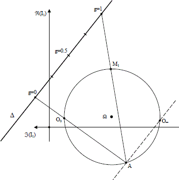
Figure 4.16. Slip graduation of the circle diagram

4.7.3. Simplified circle diagram
4.7.3.1. General introduction
This diagram is called “simplified” because it is based on the hypothesis that the stator Joule losses are negligible. It is therefore assumed that R1 = 0 all along this section. The stator current is therefore written:
[4.24] 
If the machine is assumed to be supplied by constant stator voltage ![]() , this voltage can be taken as the origin of the phases. The affixes of points O0 and O∞. respectively corresponding to g = 0 and to g infinite are:
, this voltage can be taken as the origin of the phases. The affixes of points O0 and O∞. respectively corresponding to g = 0 and to g infinite are:
![]()
They are two imaginary negative numbers. The circle is then centered on the imaginary axis at point Ω, for which the affix is ![]() .
.
4.7.3.2. Drawing of the circle
Experimentally, the circle is determined from two tests:
– a “no-load” test when the motor, supplied with its nominal voltage, drives no load: the slip is very small and the measured current will be assumed to be ![]() , and assumed to be
, and assumed to be ![]() lagging. Point Oo on the imaginary axis is 2 then determined. For convenience reasons, the real axis is usually drawn vertically (Figure 4.17);
lagging. Point Oo on the imaginary axis is 2 then determined. For convenience reasons, the real axis is usually drawn vertically (Figure 4.17);
– a test at standstill, with a stator voltage V1c reduced so that the corresponding current modulus I1c does not exceed the nominal current. The machine impedance is assumed to be independent from the voltage, the stator current corresponding to voltage V1 is calculated using ![]() . Point M1 corresponding to g = 1 can therefore be set down (Figure 4.17).
. Point M1 corresponding to g = 1 can therefore be set down (Figure 4.17).
Center Ω of the circle is then found at the intersection of the median OoM1 with the imaginary axis.
Figure 4.17. Simplified circle diagram

4.7.3.3. Interpretation of the diagram
Once the circle is drawn, it can be graduated in slip, as established above. We shall now show that it is possible to deduce from this diagram the main characteristics of the induction machine.
4.7.3.3.1. Absorbed powers
If we consider a point M on the circle, for which slip is g, vector OM represents the current Ī1, absorbed at the network, and for which the phase, with regard to the voltage, is φ (Figure 4.17). If n and m are respectively the projections of M on the real and imaginary axes, we obtain:
![]()
![]()
Segment mM therefore measures, providing the scale of the diagram is multiplied by 3V1, the active power absorbed at the network. This power is positive when point M is on the “upper” semi-circle (g > 0); it is negative for the “lower” semicircle (g < 0).
In the same way, segment Mn represents the reactive power absorbed at the network, which is always positive.
4.7.3.3.2. Electromagnetic torque
As all stator losses are neglected, the absorbed power is fully transmitted to the rotor. Therefore we have:
![]()
It is deduced:
![]()
Thus, thanks to another scale change, ![]() also measures the electromagnetic torque. The latter is therefore positive for the upper semi-circle and, when g varies from zero to +∞, the torque goes through its maximum Γm for point Mm corresponding to slip gm (Figure 4.14). By calling α the angle (OoO∞M), we get
also measures the electromagnetic torque. The latter is therefore positive for the upper semi-circle and, when g varies from zero to +∞, the torque goes through its maximum Γm for point Mm corresponding to slip gm (Figure 4.14). By calling α the angle (OoO∞M), we get ![]()
Point Mm relative to torque Гm corresponds to ![]() . It is deduced that:
. It is deduced that:
![]()
Furthermore, if the intersection of straight line O∞M with the real axis is called G, segment OG is proportional to the slip (the real axis can be graduated in g with O∞ as the pole). Given Gm the intersection of O∞Mm with the real axis. We therefore get:

hence:
[4.25] 
Expression [4.25] is very convenient because, if Γm and gm are known, it is very easy to calculate the torque corresponding to a given slip and vice versa.
4.7.3.3.3. Mechanical power
Absorbed power P1, considering the above made hypotheses, is completely transmitted to the rotor. It is then divided, on the one hand, in rotor Joule losses pj2 and, on the other hand, in mechanical power Pm. It is therefore interesting to separate those two values on the diagram. If the straight line bearing mM is graduated in 1/g, the pole is Oo and the origin is m. If P is the intersection of this straight line with OoM1, this point corresponds to value 1 of the graduation. We therefore have:

Going back to the power graduation, we have:
![]()
and, as a consequence:
![]()
Segment ![]() therefore represents the mechanical power produced by the induction machine, and segment
therefore represents the mechanical power produced by the induction machine, and segment ![]() , the rotor Joule losses. Straight line OoM1 that separates the mechanical power from the Joule losses is sometimes called “mechanical powers line”.
, the rotor Joule losses. Straight line OoM1 that separates the mechanical power from the Joule losses is sometimes called “mechanical powers line”.
4.7.3.3.4. Reversibility
The simplified circle diagram shows the reversibility of the induction machine: the half of the circle located below the imaginary axis corresponds to negative values of the slip and also negative values of the absorbed power P1. It is therefore an asynchronous generator operating with a rotation speed Ω greater than ΩS.
We shall come back to this working mode in more detail (section 4.9.2) but it is clear that, even when P1 becomes negative (point M'), Q1 remains positive, and the reactive power will therefore have to be supplied to the induction so that it is able to operate as a generator.
4.8. Induction machine characteristics
In order to illustrate the various curves of the following paragraphs, we shall consider a machine defined by:
– Pn = 1MW;
– Un = 5,000 V phase-to-phase voltage;
– 2p = 8;
– f = 50 Hz;
– gn = 1.2%;
– σ = 6.4%;
– R1 = 0.0437 Ω;
– R2 = 0.0437 Ω;
– L1 = 0.263 H;
– L2 = 0.0435 H.
Mn shall be placed on each curve point, corresponding to the nominal load of the machine. The characteristics of Figures 4.18 to 4.24 have been drawn numerically directly using the corresponding analytical equations.
Figure 4.18. Circle diagram. It can be noticed that for this machine,points M1 and O∞ are near the imaginary axis, and that the starting torque is clearly smaller than the nominal torque

Figure 4.19. Torque-slip characteristic. It can be noticed that slip gm, which corresponds to the maximum torque value, is equal to 5% with gn=1.2%

Figure 4.20. Stator-slip current characteristic
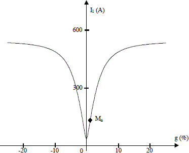
Figure 4.21. Power-slip factor characteristic. Note that in this particular case the maximum power factor corresponds to the nominal power factor

Figure 4.22. Powers-slip characteristics (P1: absorbed, P2: converted, Pm: mechanical). Note that the 3 curves almost join one another on the useful part of these characteristics (g∈ [0, gn])

Figure 4.23. Joule losses–slip characteristics (pj1: at the stator, pj2: at the rotor)

Figure 4.24. Synchronous impedance-slip characteristic
4.9. Implementation of induction machines
The use of induction machines has changed considerably over recent years. They are mainly used as motors but the number of induction generators is now increasing in the area of renewable energy particularly in wind power stations.
4.9.1. Motor mode
The induction motor is widely used in every industrial domain and for various applications, going from fixed-speed pumping (power supply by a constant frequency network) to rail traction and ship propulsion (power supply by static converters). We shall survey the various implementations starting with the most traditional one.
4.9.1.1. Constant voltage and frequency power supply
In this case, the induction motor is directly supplied by the network at an industrial frequency and drives a mechanical load the rotation speed of which is nearly constant, g being small. In such implementations, the only problem to be solved is the starting of the motor. For this analysis, the circle diagram is a good analysis support.
Referring to Figure 4.18, we can notice that when the motor is stopped (g = 1), torque Γ(g = 1) is smaller than nominal torque Γn, and absorbed current I1(g = 1) is obviously greater than the stator nominal current. This example shows that it is usually impossible to start a loaded induction motor supplied with its nominal voltage.
In order to resolve this problem, solutions vary depending on whether we are dealing with a squirrel induction motor or with a wound-rotor induction motor.
4.9.1.1.1. Squirrel induction motors
Squirrel induction motors are very robust machines, likely to support a current largely greater than their nominal current during the few seconds necessary to their starting. It is possible to reduce this current in supplying the stator with reduced voltage (star-delta connection, use of a self-transformer or of an electronic AC power controller).
The star-delta start consists of star coupling (at the time of start) a motor designed for delta working. The phase voltage is thus reduced, and therefore the starting current with a ratio of ![]() .
.
Note that, since the electromagnetic torque is proportional to the square of the voltage, if the voltage is reduced (and therefore the current) in a k ratio, the torque is ipso facto reduced in a k2 ratio. This process is therefore only to be used for no-load starting motors.
In order to improve the motor characteristics at starting, deep slots are used (Figure 4.25). Initially, the rotor frequency is equal to the supply frequency, and the skin-effect phenomenon leads to an induced current repartition concentrated at the surface of the rotor bars. This gives an increase of the apparent resistance of the bars, that is to say an increase in resistance R2, and therefore a decrease in the starting current. On the circle diagram gm moves and provides an increase of the starting torque. With the increase of speed, the rotor frequency decreases, the skin depth increases and leads to the reduction of the rotor resistance.
Various slot shapes can be used. It is clear that, for instance, in adopting trapezoid slots (Figures 4.25b), the variation effect of the resistance increases. At 50 Hz and for aluminum bars, it can be shown that this effect is noticeable only for bar heights over 2 cm.
Double-cage rotors are also used (Figure 4.26) in order to improve the starting performances of the machine. The first cage, or starting cage, is set near the air-gap. Its resistance is great due to the choice of the section and of the materials the bars are made from. Furthermore, its setting near the air-gap gives it a small leakage reactance. On the contrary, the second cage, or inside cage, is characterized by a smaller resistance and a greater leakage reactance.
Initially, both cage resistances are smaller than their reactances, and the induced currents are almost restricted to the outer cage, characterized by the smaller inductance. The starting torque is therefore great, and the current, reduced. In nominal working, the rotor frequency is small and the bars reactances become smaller than their resistances. The induced currents are then concentrated in the small resistance inner cage. The corresponding slip is then small, which leads to a good efficiency.
Figure 4.25. Deep slots: a) rectangular; b) trapezoid

Figure 4.26. Slot bearing a double cage

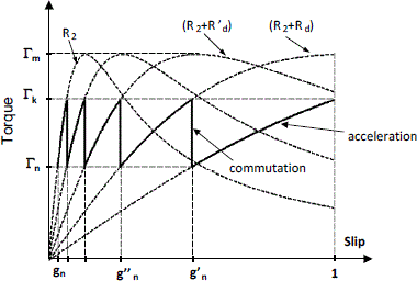
4.9.1.1.2. Wound-rotor induction motors
When induction motors have wound rotors, it is possible to connect their rotor phases, star coupled, to external resistances through slip-rings and brushes (Figure 4.2). Those resistances called “starting rheostats” enable us to modify the apparent value of resistance R2 (Figure 4.27) This starting method is almost not used any more. However we are introducing it because of its historical and pedagogical interest.
Figure 4.27. Rotor starting rheostat

The starting values of the motor (torque and absorbed current) can be modified in this way. Indeed, if the induction machine equations are considered, it is clear that (equation [4.23]) absorbed current I1 depends on the slip through term ![]() , that is to say that (V1 and f being fixed) a working point is related to a
, that is to say that (V1 and f being fixed) a working point is related to a ![]() ratio. Furthermore, maximum torque
ratio. Furthermore, maximum torque ![]() does not depend on R2, but the corresponding slip
does not depend on R2, but the corresponding slip ![]() is proportional to R2.
is proportional to R2.
The circle diagram is a good reasoning support to show the influence of the starting rheostat (Figure 4.28). Let us assume that the machine under consideration can endure a starting current kIn and has to drive a load for which the resistant torque is equal to nominal torque Γn. On the circle the corresponding points are respectively Mk and Mn. Point M1 of slip g = 1 (without a rheostat) is also noted.
Figure 4.28. Circle diagram

Calling gk the slip corresponding to Mk in normal working, it is possible to set down the starting point in Mk provided that a rheostat of resistance Rd is used:
![]()
hence:
[4.26] ![]()
If the corresponding starting torque Γk is greater than Γn, the motor starts, accelerates, and its working point follows arc MkMn. Its speed stabilizes for a slip g’n corresponding to point Mn (torque Γn). It can be written:
![]()
The previous calculation can be taken again in order to place the point with slip g'n in Mk and to calculate the new rheostat resistance R'd:
![]()
In commutating the rheostat from Rd to R'd, the move from Mn to Mk is instantaneous and the motor accelerates again to go back to Mn, and so on and so forth. In plane Γ(g), the characteristics of Figure 4.29 are obtained.
Figure 4.29. Torque variation at starting
4.9.1.2. Variable voltage and fixed frequency supply
We shall see in the following (section 4.9.1.3) that the most effective way to vary the speed of an induction motor consists of varying the frequency of the supply. However, for small power and low cost applications, another solution consists of varying the rms value of the supply voltage only.
In order to grasp the principle of this approach, it is suitable to refer to the torque-slip characteristic of the machine (equation [4.19] and Figure 4.13). If it is assumed that, for example, the motor drives a load of torque ΓC(g), the working point will be at the stable intersection of those two characteristics (Figure 4.14). If these characteristics are drawn for various values of V1, a family of curves Γ(g) deduced by homothetic transformation and with their maxima for the same value gm of g is obtained (Figure 4.30). Their intersections with torque ΓC line therefore correspond to slips g, g', g'', etc. which are larger when voltage V1 is small. It is therefore possible in this way to vary, in a relatively small range, the induction motor speed. In order for this range to be as wide as possible, it is advisable to use motors with their maximum torque Γm for important values of the slip. Their rotor resistance R2 therefore has to be significant. For this kind of application, machines with highly resistive cages are therefore used.
This variable voltage power supply is usually made using a 3-phase electronic AC power controller (Figure 4.31).
Figure 4.30. Torque-slip characteristic for various stator voltages

Figure 4.31. 3-phase electronic AC power controller supply

It will be noted that, as this speed variation is based on a slip increase, it leads to a considerable decrease of efficiency η since η < (1 - g). Moreover, electronic AC power controller supply generates non-sinusoidal currents, and harmonics contribute still further to reduce efficiency. That is why this way is only used for small power cage induction motors, destined to low-cost applications: pumps, fans, etc.
4.9.1.3. Variable frequency and voltage supply
This is the most modern and the most high-performance method of induction machine implementation. It was made possible by the emergence of voltage source inverters (Figure 4.32) at the end of the 1960s, then by their continued increase in power and performance. The principle of this implementation mode of induction motors follows from the expression:
![]()
which shows that, if the slip is small, the speed is almost proportional to the stator angular frequency, and therefore to the frequency.
In supplying the stator with variable frequency voltages, it is therefore possible to control the machine speed. It is however advisable to make these voltage amplitudes vary according to frequency.
Figure 4.32. Variable frequency drive

We shall, in the following, first deal with the problem using a simplified approach overlooking the stator resistance.
4.9.1.3.1. Constant V1/f supply
If R1 is neglected, impedance ![]() is written:
is written:
![]()
with ωr = gω.
The expression of the absorbed stator current can therefore be deduced:
[4.27] 
This expression shows that if a constant ratio V1/ω is imposed when frequency varies, the current absorbed at the stator depends only on rotor angular frequency ωr.
4.9.1.3.2. Circular diagram
Expression [4.27] defines, for a stator current, a Möbius function of variable ωr in the complex plane. The extremity N of the vector with the affix Ī1 therefore describes a circle when ωr varies from –∞ to +∞. This circle is centered on the imaginary axis in the middle Ω of segment N0N∞ points respectively corresponding to the rotor angular frequencies ωr = 0 and ωr→ ∞ (Figure 4.33).
This circle can, in the same way as the standard circle diagram, represent the powers exchanged with the source and the electromagnetic torque Γ. The result in particular is that segment nN represents both the absorbed active power and the torque. It is therefore deduced that characteristic Γ(ωr) is unique. We have:
[4.28] 
The torque goes through a maximum (Figure 4.34) given by:
![]()
for:
![]()
Figure 4.33. Circular diagram of the stator current: V/f constant and ωr variable

Figure 4.34. Torque variation in terms of the rotor angular frequency. Supply at constant V/f

Characteristic Γ(ωr) being unique, load torque ΓC fixes a value ωr, and therefore one and only current I1, regardless of the frequency. This approach led to the development of rustic, sturdy variable speed drives that are satisfying when considerable dynamic performances are not sought.
However it is advisable to underline the limits of this study:
– first, it calls for a “permanent state” type model of the induction machine, which restricts its validity to slow frequency variations;
– then, the simplifying hypothesis, consisting of neglecting the stator resistances, is valid only for quite high frequencies. For low frequencies (particularly at starting), it is advisable to modify slightly the variation law of V1 in terms of the frequency, in order to compensate the voltage drops due to the stator impedances. It is then called “constant flux” supply.
4.9.1.3.3. Introduction to vector control
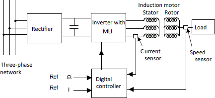
The previous study (constant V/f or constant flux supply) is a matter for an “open loop” approach to speed variation, an approach from which it would be unrealistic to expect great accuracy and considerable dynamics. If this kind of performance is sought, it is necessary to rely on another theoretical approach, based on the exploitation of the induction machine transient equations (Park equations). Very high-performance speed and current regulations can then be developed, using pulse width modulation inverters (PWM) and digital control.
The principle of this implementation is represented by Figure 4.35 where Ref Ω and Ref I respectively represent the desired speed and the maximum admissible current. These systems, called “vector control drives”, have been the subject of an abundant scientific literature over the past years. Their study goes beyond the scope of this book.
Figure 4.35. Structural diagram of a vector-controlled induction machine
4.9.2. Generator mode
Induction machines are mainly used as motors but, as with all rotating machines, they are reversible. Their use as generators has shown an increase in interest for a few years, particularly for the use of renewable energies such as wind energies.
4.9.2.1. Induction generator connected to a network
When an induction machine is connected to an electrical power network, the circle diagram is, as we have already seen, a good tool for a qualitative analysis.
Considering the diagram in Figure 4.36, it is clear that when the machine works with a negative slip (that is to say at a speed Ω > Ωs) corresponding for instance to point M', the active power represented by ![]() is negative. Angle φ is greater than π/2 and the electromagnetic torque (also represented by
is negative. Angle φ is greater than π/2 and the electromagnetic torque (also represented by ![]() ) is negative. All this characterizes a generator mode for which the machine absorbs the mechanical power (represented by
) is negative. All this characterizes a generator mode for which the machine absorbs the mechanical power (represented by ![]() ) and supplies the network with electrical power (represented by
) and supplies the network with electrical power (represented by ![]() ).
).
Figure 4.36. Simplified circle diagram. Induction generator mode

This diagram also makes a fundamental aspect of the induction machine appear: the reactive power represented by ![]() had to be supplied to the machine for generator mode and for motor mode.
had to be supplied to the machine for generator mode and for motor mode.
This operating mode is used to recover energy for cyclic working devices, for example service elevators: the induction machine operates as a motor on the way up and as a generator on the way down. On a way up-way down cycle, the overall energy consumption thus only represents losses.
Induction generators are also used in “micro-power plants” when the presence of a watercourse or of other primary energies (particularly wind energies) enables us to drive machines and supply the network.
4.9.2.2. Self-excited induction generator
The induction machine, unlike the synchronous machine, has no field winding; therefore it can produce energy only if an external source provides it with the reactive power needed for its magnetization. In isolated mode, this source is made of a capacitor bank C connected to the terminals of the stator windings (Figure 4.37).
Figure 4.37. Self-excited induction generator

When the load is zero (switch K open), the equivalent diagram per phase is given in Figure 4.38.
Figure 4.38. Per phase equivalent circuit of a self-excited induction generator

In driving the rotor at speed Ω, the self-voltage build-up is possible if capacitor C provides a reactive energy Qc equal to the sum of QL1 and Qn2 absorbed by inductances L1 and N'2. If the voltage drop in stator resistance R1 is neglected, Qc and Ql1 can be written in terms of V1:
![]()
QN'2 is usually small, hence the necessary condition of no-load self-voltage build-up:
QC > QL1
which leads to L1Cω2 > 1. The minimum values of C in terms of L1 can thus be determined. Angular frequency ω is almost equal to pΩ.
In order to explain the self-voltage build-up phenomenon, it is necessary to take into account the saturation as well as the remanence field in the magnetic circuit. Those phenomena are complex, and we shall restrict to qualitative explanations in the following analysis.
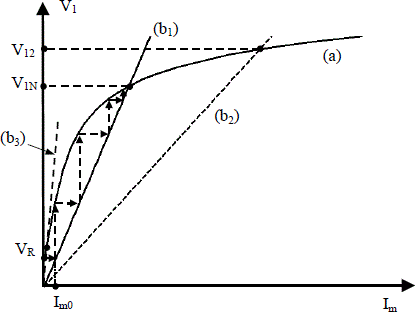
Figure 4.39 shows that when the machine is driven by an external device, the remanence field of the rotor generates an emf VR at the terminals of each stator phase, leading to the creation of a reactive current Im0. This magnetizing current increases the flux in the machine, which increases the voltage of phase V1. In a no-load state, the modulus of V1 is related to the magnetizing current Im through the specific internal magnetic characteristic of the machine V1(Im) (Figure 4.39, curve a), and also through external characteristic ![]() (curve b1). The operating point is therefore obtained by the intersection of these two characteristics.
(curve b1). The operating point is therefore obtained by the intersection of these two characteristics.
Figure 4.39, representing the evolution of current Im during the self-voltage build-up, shows that the value of C can be chosen so that the working point corresponds to nominal voltage V1n (curve b1). It also shows that when the value of C is important (leading to a low slope of the external characteristic), the working point corresponds to a great voltage V12 that can be dangerous for the machine (curve b2). It is furthermore deduced that if the value of C is too small, there cannot be any self-voltage build-up (curve b3).
Figure 4.39. Voltage build-up in a self-excited induction generator
Let us consider the case when the generator supplies an inductive load Z (Figure 4.38, switch K closed). When the load increases, the capacitor value has to increase in order to maintain the desired frequency and voltage because, on the one hand, the reactive energy needed by the machine increases, and, on the other hand, C also has to provide the reactive energy for Z.
The value of the capacitor needed for the working can be obtained by writing the two equations relative to energy conservation:
– the reactive energy generated by the capacitor bank is equal to this absorbed by inductances L1, N'2 and the imaginary part of Z;
– active energy ![]() is consumed in resistances R1 and the real part of Z.
is consumed in resistances R1 and the real part of Z.
We shall not develop this calculation in this book.
Figure 4.40 shows, at a given frequency, the evolution of the phase voltage in terms of the active power P provided by the generator for various values of capacitor C, with C1 < C2 < C3.
Figure 4.40. Voltage-power characteristics for various capacitors (C1 < C2 < C3)

In order to maintain a fixed frequency when the load increases, that is to say when the slip increases, the generator speed Ω has to be increased slightly:
![]()
Note that when P increases, the voltage given by the machine decreases faster for smaller values of C. For a small capacitor value, for example C = C1, note that power P goes through a maximum and then diminishes. In this case, if the call for power is maintained it can bring about the demagnetization of the generator and lead to its working stop.
Figure 4.40 also shows that, in order to regulate the voltage at the load terminals, when P increases, the reactive power issued by capacitor bank C has to increase.
4.9.2.3. Doubly-fed induction machine
So far we have considered that the rotor currents were induced in the short-circuited coils. It is obvious that for cage motors, there is no alternative, but for the wound rotor machines, it is possible to inject a 3-phase AC current system of fundamental frequency fr into the rotor. These rotor currents are produced by an inverter working in pulse width modulation while the machine stator is connected to the network of angular frequency ω. It is then called a “doubly-fed induction machine” or a “DFIM” (Figure 4.41).
This system working principle and its uses can be deduced from expression [2.12], which is revised here:
![]()
If ω is considered to be constant, we can note that in fixing angular frequency ωr, speed ![]() is set. This is used for quite economical rotation speed variators because the static converters only have to supply the rotor power.
is set. This is used for quite economical rotation speed variators because the static converters only have to supply the rotor power.
Figure 4.41. Doubly-fed induction machine principle
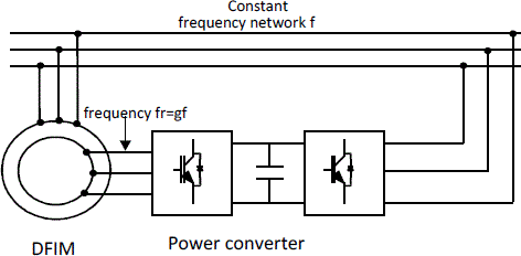
The main application of this drive is energy production made from wind energy. Indeed, in this case, rotation speed Ω. is linked to the speed of the wind, and therefore is highly variable. If AC generators are used, the frequency of the obtained voltages is therefore also variable, which does not allow us to connect them directly to the network.
On the contrary, for the DFIM, the rotor windings only have to be supplied with an angular frequency ωr = ω – pΩ in order to obtain the desired stator frequency regardless of the rotor rotation speed. It is therefore possible to connect the DFIM directly on the network.
Figure 4.42. Doubly-fed induction machine wind turbine (parc de Bouin, Vendée, France). 2.5 MW, 660 V machines. The three-bladed turbine has a diameter of 80 m, and its speed is between 11 and 19 rpm. The generator rotation speed is near 1,500 rpm. The induction machine is connected to the blades by a mechanical device multiplying the speed

4.9.3. Single-phase induction motor
When a 3-phase source is not available, single-phase induction motors are often called upon to drive small-power devices (pumps, fans, compressors, etc.).
4.9.3.1. Structure
A single-phase induction motor is a cage induction motor, for which the stator has the same structure as the stator of a 3-phase motor, but where only 2/3 of the slots are used to make a single-phase winding. The additional 1/3 enables the winding of a so-called “auxiliary” phase, used for starting, as we shall see in the following.
In an initial analysis, a single-phase induction machine can be considered as a 3-phase machine supplied by a single-phase current at the stator with voltage U (Figure 4.43).
Figure 4.43. Single-phase power supply of the induction machine

4.9.3.2. Equations
According to the previous section, it can be considered, for example, that the current in phase A is equal to zero and that ![]() . Furthermore it is also possible to write
. Furthermore it is also possible to write ![]() .
.
We are in the presence of a problem with an induction machine in an unbalanced operating mode, and Fortescue's symmetrical components method is very convenient for analyzing it (see section 1.2.4).
4.9.3.3. Stator current calculation
The stator supply voltage U is assumed to be known, and the machine impedances in direct, inverse and zero-sequence modes are called Zd, Zi and Zo. We therefore have the six expressions, on the one hand:

in the phase value scale, and on the other hand:

in Fortescue's component space.
It is advisable to incorporate the previous equations when using the passage expressions:

We therefore obtain:
[4.29] 
After calculation, the three currents and the three voltage expressions in Fortescue's space are deduced:
[4.30] 
[4.31] 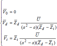
If the inverse transformation is used to calculate the phase values, we finally obtain:
[4.32] ![]()
This expression enables us to calculate the absorbed stator current, providing ![]() and
and ![]() are known.
are known.
4.9.3.4. Positive and negative sequence impedances of the induction machine
![]() and
and ![]() are, by definition, the impedances presented by the induction machine to respectively positive and negative sequence current systems. The words “positive sequence” and “negative sequence” can be interpreted in relation to the rotor rotation direction.
are, by definition, the impedances presented by the induction machine to respectively positive and negative sequence current systems. The words “positive sequence” and “negative sequence” can be interpreted in relation to the rotor rotation direction.
It is therefore possible, by respectively naming gd and gi the rotor slips corresponding to the positive sequence and negative sequence rotating fields, to write:
![]()
If the phase impedance expression is considered again, we obtain:
[4.33] ![]()
[4.34] ![]()
If these expressions are transferred into expression [4.32], the variation of stator current I in terms of slip g can be deduced.
4.9.3.5. Single-phase induction machine torque
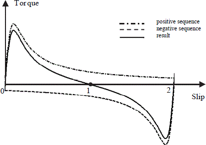
The single-phase induction machine torque is the resultant of torque Γd due to the positive sequence currents component and to torque Γi linked to the negative sequence component. Γi is a braking torque:
![]()
In referring to expression [4.19] and to Figure 4.12, we get:
[4.35] 
[4.36] 
If expressions [4.35] and [4.36] in connection with [4.31], [4.33] and [4.34] are considered, it is clear that torque Γ has a symmetrical formulation in terms of g and (2 – g). The characteristic of Figure 4.44 shows the variation in terms of the slip of positive sequence and negative sequence torques. The resultant torque can then be deduced. This characteristic Γ(g) emphasizes:
– the symmetry in terms of the point corresponding to g = 1. The motor therefore has no favorite rotation direction;
– the cancellation of the torque for two values of the slip, one slightly below 0, and the other, worth 2;
– a value of the torque developed by the single-phase motor, for a given slip, smaller than this of the 3-phase motor;
– cancellation of the resultant torque for g = 1. The single-phase asynchronous motor therefore does not start by itself. Specific methods are needed for it to start.
Figure 4.44. Single-phase induction machine torque
4.9.3.6. Capacitive single-phase motor
The stator winding of the single-phase induction machine usually takes only 2/3 of the slots. It is therefore possible to use the remaining slots to make an auxiliary coil PA shifted of π/2 electrical in terms of the main winding called PP.
In supplying the main winding with a single AC current IPP, the motor cannot start because the corresponding field is pulsating. We then seek to generate a rotating field in the motor in supplying simultaneously PA and PP, so that current Ipa in the auxiliary winding is shifted from IPP.
This phase-shift can be obtained by adding an impedance in series with the auxiliary winding. This impedance can be, in some cases, a resistance or an inductance, but a capacitor is usually used.
The aim is to obtain (or to approach) the equivalent of a balanced 2-phase motor that produces a circular rotating field. Coils PP and PA being shifted in space of π/2 electrical, it would be necessary that for all the rotation speeds, magnetomotive forces NPPIPP and NpaIpa (NPP and NPA respectively being the number of turns of phases Pp and Pa) are equal and shifted in time of π/2 electrical. This constraint is very hard to achieve in practical terms.
Let us consider the diagram of the capacitive motor given by Figure 4.45a. Voltage V1 is applied to main phase Pp and to auxiliary phase PA in series with capacitor Cp.
When speed varies the impedances of coils Pp and Pa also vary, leading to the variations of the magnitudes and the phases of currents Ipa and Ipp. Thus, for example, if a value of C provides a circular rotating field at the start of the motor is chosen, the mmf NppIpp and NpaIpa will no longer be equal and shifted by π/2 electrical for a speed that is different from zero. For this speed, the corresponding field would therefore not be circular. It is called elliptic, because the locus of the vector representing at every instant the maximum field is an ellipse.
The elliptic field can be broken into two circular fields rotating in opposite directions. The field rotating in the positive sequence direction (rotation direction) produces the useful torque while the negative sequence field generates a harmful braking torque.
Single-phase induction motors are used to drive devices for which power usually does not go over a few kW. Permanent capacitor motors Cp (Figure 4.45a), start capacitor motors Cd (Figure 4.45b) or start capacitor and permanent capacitor motors (Figure 4.45c) are encountered.
The standard permanent capacitor motor is reserved for small-power uses enabling a starting torque smaller than the nominal torque. The auxiliary phase is permanently in series with capacitor Cp.
In order to increase the starting torque, a capacitor of larger capacity is used for an “intermittent duty”. When speed reaches about 2/3 of the nominal speed, a centrifugal contactor K (or electric relay) connected in series with the auxiliary phase opens and cuts the starting circuit. The nominal working is then solely single-phase (only one coils is power-supplied) and characterized, as we have seen previously, by the presence of an inverse braking torque and a poor power factor.
At the same time, in order to improve the starting torque, the power factor and the efficiency, start capacitor and permanent capacitor motors (Figure 4.45c) are adopted. At the start, the two capacitors Cd and Cp are connected in parallel and the total capacity (Cd + Cp) is chosen so that the motor produces a torque about twice the nominal torque.
Figure 4.45. Single-phase motor: a) permanent capacitor; b) start capacitor; c) permanent capacitor and start capacitor

After the start, the “intermittent” capacitor Cd is disconnected beyond a particular speed thanks to Switch K. Permanent capacitor Cp is chosen so that the permanent working is almost of the same as a balanced two-phase motor characterized by a small slip (that is to say a good efficiency) and a good power factor.
For these three kinds of motors, the inversion of the rotation direction is obtained by changing the connections of one phase.
4.10. Principle of the experimental determination of the parameters
The determination of the parameters appearing on the equivalent diagrams is necessary for the predetermination of the machine characteristics. This determination is quite different depending on whether it is a wound rotor induction machine or a cage induction machine, especially concerning the rotor parameters. Let us consider the equivalent figure given in Figure 4.46. This corresponds to Figure 4.10a to which a resistance Rf representing the iron losses is added.
Figure 4.46. Equivalent diagram per phase including iron losses

4.10.1. Case of wound rotor induction machines
In this case, all the parameters can be obtained through direct measurement. Stator and rotor resistances are measured in DC current using an “ammeter-voltmeter” method (nominal temperature and current).
Stator leakage inductance L1 can be measured directly by leaving the rotor circuit open. It is usually preferable to make a no-load test, with a “zero” slip motor.
Voltage and phase current V10 and I10, are measured as well as active and reactive powers P10 and Q10 absorbed by the machine. L1 and Rf are then deduced using:
![]()
In the same way, inductance L2 can be obtained via a test by supplying the rotor with a 3e-phase system, when the stator is in open circuit. The value of the induced voltage on the non-supplied side gives two measurements of the “transformation ratio”,![]() , enabling us to determine
, enabling us to determine
M
4.10.2. Case of cage induction machines
It is neither possible to directly access the rotor parameters nor to leave the rotor in open circuit. Stator resistance R1 is measurable directly in DC current, and inductance L1 is deduced from a no-load test (g ~ 0).
As for the wound rotor induction machine, L1 and Rf are determined from the measurement of voltage and phase current, V10 and I10, and from the active and reactive powers P10 and Q10 absorbed by the machine.
Concerning the rotor parameters, determination can only be indirect. A test with a locked rotor (g = 1), under reduced voltage, enables (knowing L1 and R1 which can often be neglected) us to determine elements N'2ω and R'2 appearing on the equivalent diagram of Figure 4.46. With g = 1, it can indeed be admitted that:
![]()
I1c, P1c and Q1c are respectively the current and the active and reactive powers absorbed by the machine.