Chapter 1
Main Requirements
1.1. Introduction
The study of rotating electrical machines is a science which is linked with several other topics. In order to make this book easier to read, we are going to summarize the main results and concepts used later on in this introductory chapter:
– sinusoidal systems;
– electromagnetism;
– power electronics.
1.2. Sinusoidal variables
1.2.1. Single-phase variables
1.2.1.1. Timed expressions
An x variable, a timed-sinusoidal function, can be written as:
![]()
where X is the rms (root-mean-square) value and is the angular velocity.
1.2.1.2. Vector representation
The x variable defined above can be considered to be the projection on an axis of a vector of length X![]() rotating anticlockwise at an angular velocity ω (Figure 1.1).
rotating anticlockwise at an angular velocity ω (Figure 1.1).
Figure 1.1. Vector representation of a sinusoidal variable

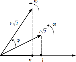
1.2.1.3. Single-phase currents and voltages
If a sinusoidal single-phase voltage v is applied at a Z impedance terminal, current i in this impedance, at steady state, is also sinusoidal, and can be written:
![]()
![]()
φ being the phase shift between the voltage often chosen as the origin and the current. Conventionally, φ is counted positively when the current is lagging behind the voltage. The instantaneous power supplied to impedance Z is:
![]()
[1.1] ![]()
is the active power and:
[1.2] ![]()
is the pulsating power. It must be noted that this variable, which characterizes the fact that the single-phase power supplied to a receiver is time varying, is cancelled with balanced polyphase systems.
Figure 1.2 shows that voltage is changed into current through a similitude of ratio Z and angle φ.
Figure 1.2. Vector representation of sinusoidal current and voltage
1.2.1.4. Complex representation
Complex numbers are very useful to represent the previous similitude and vector ![]() will thus be associated with complex number
will thus be associated with complex number ![]() as well as complex number Ī with vector
as well as complex number Ī with vector ![]() . They can then be written as follows:
. They can then be written as follows:
![]()
![]()
Complex impedance ![]() is also defined by ratio:
is also defined by ratio:
![]()
It will be set down:
![]()
![]()
R and X respectively being the resistance and the reactance expressed in Ohms.
![]() is also introduced :
is also introduced :
[1.3] ![]()
![]() is the apparent power expressed in volt-amperes (VA). Q is the reactive power expressed in volt-amperes reactives (VAr).
is the apparent power expressed in volt-amperes (VA). Q is the reactive power expressed in volt-amperes reactives (VAr).
1.2.2. 2-phase voltages and currents
A 2-phase voltage system is defined by two voltages in quadrature:
![]()
![]()
if it is loaded onto a symmetrical impedance it leads to a balanced 2-phase current system:
![]()
![]()
There is no pulsating power and the instantaneous power is constant:
![]()
Figure 1.3. 2-phase currents and voltages

The complex representation can also be introduced:
![]()
![]()
with the expressions of the active and reactive powers:
![]()
![]()
1.2.3. Balanced 3-phase sinusoidal systems
1.2.3.1. Time expressions
A balanced 3-phase voltage system is composed of three voltages with the same frequency, with the same amplitude and phase shifted by a third of a period with respect to the others. It is thus written as a time expression:

If this voltage system is connected to a symmetrical load (with a circulating impedance matrix), it leads to a balanced current system (Figures 1.4 and 1.5):

with the vector representation shown in Figure 1.4.
Figure 1.4. 3-phase currents and voltages

A zero pulsating power is then obtained and the instantaneous power is constant and equal to the active power:
![]()
1.2.3.2. Associated complex notations
Complex vectors are associated with balanced voltage and current systems:
[1.4] 
where 1, a and a2 are the cube roots of the unit: a=e j2π/3 , a2 = e j4π/3.
If the 3-phase voltage system is applied to a load characterized by a circulating impedance matrix ![]() (Figure 1.5) such as:
(Figure 1.5) such as:

the expression ![]() leads to the phase equation:
leads to the phase equation:
![]()
in which:
[1.5] ![]()
is the impedance of the load.
Figure 1.5. Balanced 3-phase load

This happens as if each of the three phases was loaded with a ![]() impedance decoupled from the other two (it is in fact a diagonalization of the impedance matrix that has
impedance decoupled from the other two (it is in fact a diagonalization of the impedance matrix that has ![]() as an eigenvalue). In those conditions balanced 3-phase systems can be dealt with as independent and decoupled single-phase systems.
as an eigenvalue). In those conditions balanced 3-phase systems can be dealt with as independent and decoupled single-phase systems.
1.2.4. Unbalanced 3-phase sinusoidal systems: Fortescue symmetrical components
Voltage and current systems may be unbalanced (different amplitudes depending on the phases or phase-shifts different from 2π/3). Expressions [1.4] and [1.5] are no longer valid and 3-phase equations cannot be replaced by single-phase equations. Generally, the analysis of these systems is very difficult.
However there is a system class, fortunately quite commonplace in electrical engineering, for which there is a mathematical simplification. They are the devices described by a circulating impedance matrix ![]() and to which dissymmetrical external conditions are imposed. It can be demonstrated that matrix
and to which dissymmetrical external conditions are imposed. It can be demonstrated that matrix ![]() has three eigenvectors:
has three eigenvectors:
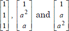
respectively associated with the three eigenvalues:
[1.6] ![]()
[1.7] ![]()
[1.8] ![]()
The three above-written impedances are respectively called zero phase-sequence impedance, forward impedance and backward impedance. A transformation matrix can be built from the three eigenvectors:
[1.9] 
called “Fortescue's matrix”. Its backward matrix is:
[1.10] 
If three variables composing an unbalanced 3-phase system are named Ga, Gb and Gc (voltages, currents, flux, etc.), then the homologous variables G0, Gd and Gi can be defined by:
[1.11] 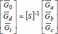
with, of course, the opposite transition expression:
[1.12] 
This last expression shows that if only the forward (positive phase-sequence) part exists, the above-mentioned balanced 3-phase system (Figure 1.4) will be found:

only if the backward (negative phase-sequence) part is not zero:

A balanced 3-phase system is obtained, also known as “backward (negative phase-sequence)”, for which components b and c exchange their roles.
Finally, if only ![]() is different from zero:
is different from zero:

This is an expression defining a zero phase-sequence 3-phase system in which the three components are identical.
Figure 1.6. Systems: a) forward (positive phase-sequence); b) backward (negative phase-sequence); c) zero phase-sequence

This approach therefore consists of replacing an unbalanced 3-phase system with the superposition of three different balanced 3-phase systems of different natures: forward, backward and zero phase-sequence, which can be studied separately and easily.
Matrix equation:
![]()
in which ![]() and
and ![]() represent voltage and current unbalanced systems, can be divided into:
represent voltage and current unbalanced systems, can be divided into:

![]() and
and ![]() are respectively the impedances of the device in zero phase-sequence, forward and backward modes.
are respectively the impedances of the device in zero phase-sequence, forward and backward modes.
This method, called “Fortescue's symmetric components”, is very convenient for studying and calculating unbalanced sinusoidal 3-phase systems. It is also noticeable that it can be used to study non-sinusoidal balanced 3-phase systems. Indeed it can be demonstrated that 3k rank harmonics create zero phase-sequence systems, that 3k + 1 rank harmonics create forward systems and that 3k - 1 rank harmonics create backward systems.
1.3. Electromagnetism
1.3.1. Primary laws
1.3.1.1. Maxwell's equations
Considering the industrial frequencies used in power systems, displacement currents ![]() are neglected, and Maxwell's equations can be written as follows:
are neglected, and Maxwell's equations can be written as follows:
[1.13] ![]()
[1.14] ![]()
[1.15] ![]()
[1.16] ![]()
E [V/m] and H [A/m] are respectively electric and magnetic fields. D [C/m2] and B [T] are the electric flux density and the magnetic flux density. J [A/m2] is the current density, and ρ [C/m3] the volume charge density. Equation [1.13] illustrates the coupling between E and B, whereas equation [1.14] leads to div ![]() = 0 (i.e.nodal rule). Equations [1.13] to [1.16] are valid in any fixed or mobile axis systems provided the different variables are measured and their derived values are calculated in the same coordinate system. Considering the speeds encountered in power systems, H, B and J are unchanged in a reference frame moving at speed
= 0 (i.e.nodal rule). Equations [1.13] to [1.16] are valid in any fixed or mobile axis systems provided the different variables are measured and their derived values are calculated in the same coordinate system. Considering the speeds encountered in power systems, H, B and J are unchanged in a reference frame moving at speed ![]() . Only the electric field is modified as follows:
. Only the electric field is modified as follows:
[1.17] ![]()
1.3.1.2. Ampere's theorem
Equation [1.14] leads to:
[1.18] ![]()
The magnetic field circulation on a closed circuit (C) is equal to the algebraic sum of the embraced currents.
1.3.1.3. Faraday's law
Let's consider circuit (C) in Figure 1.7, first assumed to be fixed. Equation [1.13] leads to:
[1.19] ![]()
ϕ is the magnetic flux through circuit (C)'s surface S and e is the induced electromotive force (emf) on (C)'s terminals. This is a transformation emf.
If (C) is moving at speed ![]() , equation [1.17] gives:
, equation [1.17] gives:
[1.20] ![]()
The induced emf at (C)'s terminals is the sum of the transformation emf eT and of emf eV, also called speed emf or emf due to the cut-flux.
Figure 1.7. Production of an emf at the circuit's terminals

1.3.2. Materials and magnetic circuits
When a material is subjected to a magnetic field H, each dV element gains a magnetic moment able to oppose or add itself to H. Those magnetic moments can be considerable for ferromagnetic materials. Magnetic flux density within the material is written:
![]()
μ0![]() is the flux density which would have been created into free space, and
is the flux density which would have been created into free space, and ![]() [A/m] is the magnetization. This is noted:
[A/m] is the magnetization. This is noted:
![]()
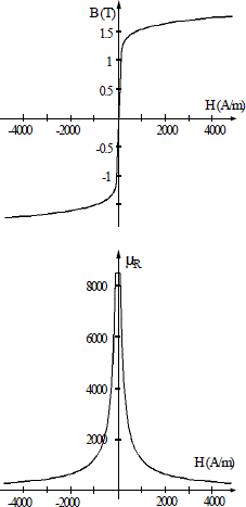
The magnetic susceptibility χ usually varies in a very complex way with the field and leads to a B(H) expression presenting a hysteresis (Figure 1.8). Figure 1.8 shows the remanence flux density Br, the coercive field Hc and the initial magnetization characteristics.
According to the hysteresis cycle, “soft” materials can be distinguished from “hard” materials. Soft materials (electrical steel, solid steel, etc.) are characterized by a narrow cycle. Br and Hc are weak. Hc is around 50 to 70 A/m, whereas Br is below 0.1 T. Hard materials (permanent magnets) have a wide cycle. The coercive field Hc is held between 200 and 1,000 kA/m while Br is held between 0.3 T and 1.2 T.
Figure 1.8. Hysteresis cycle

1.3.2.1. Soft ferromagnetic materials
As the hysteresis cycle is narrow, only the initial magnetization curve is taken into consideration. If the material is characterized by a constant χ
![]()
µR = 1 + χ is the relative permeability.µ is the material's permeability [H/m]. The ferromagnetic materials are characterized by X ≈ χµR>> 1. The magnetic materials have a susceptibility close to zero. This is negative (χ-10-5 for the diamagnetic materials and positive (χ=10-3) for the paramagnetic materials.
1.3.2.1.1. Saturation
The magnetic permeability of ferromagnetic materials depends on the applied field:
![]()
Figure 1.9 shows the initial magnetization curve as well as the relative permeability in terms of the magnetic field of a steel frequently used in electrical machines.
Figure 1.9. Initial magnetization curve and variation of the relative permeability of FeV 400-50 HA steel in terms of the field
1.3.2.1.2. Iron losses
Hysteresis losses
When the field in a ferromagnetic material varies with time, losses (called hysteresis losses) appear; they are proportional to the area enclosed by this hysteresis loop. They correspond to the energy required for the orientation of the magnetic moments. Those losses are proportional to frequency f of the excitation currents, as well as to volume V of the magnetic circuit:
![]()
Bm is the maximum value of the magnetic flux density. Constant Kh depends on the material. n is the Steinmetz coefficient; its value is held between 1.8 and 2. The value n = 2 is often accepted.
Eddy current losses
Let us consider the solid ferromagnetic circuit drawn in Figure 1.10.
Figure 1.10. Flux and induced currents in a solid circuit

When mmf (i.e. magnetomotive force) NI is variable, currents are induced in the conductive iron. The corresponding losses are called “eddy current losses”. In order to reduce those losses the solid material is usually replaced by thin metal sheets insulated from one another. Those losses are given by:
![]()
Constant KF depends on the material, e is the metal sheet thickness (about 0.5 mm for electrical machines).
Iron losses
The sum of the hysteresis losses and the eddy current losses are usually gathered under the name “iron losses” (Pfer):
![]()
1.3.2.1.3. Magnetic circuits
We have seen that ferromagnetic materials are characterized by an important permeability which enable the magnetic flux to be canalized.
Hopkinson's law
Let us consider the circuit characterized by the average closed path (C) of length l (Figure 1.11). Assuming that field ![]() and
and ![]() are colinear, and assuming that H is constant, Ampere's theorem leads to:
are colinear, and assuming that H is constant, Ampere's theorem leads to:
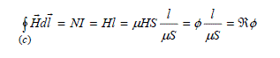
Hopkinson's law is obtained:
[1.21] ![]()
ε is the magnetomotive force, expressed in [At]. ℜ is the magnetic circuit reluctance, and ℘ its permeance, with:
[1.22] ![]()
Figure 1.11. Magnetic field and average flux path

Analogy between a magnetic circuit and an electrical circuit
Hopkinson's law can be represented by Figure 1.12. The flux ϕ circulates within reluctance ℜ of the magnetic circuit, like current I which circulates within resistance R of the electrical circuit. In comparison to Ohm's law, it is therefore noted that mmf ε, flux ϕ and reluctance ℜ are respectively similar to voltage V, current I and electrical resistance R. However there is no equivalence to the notion of electrical losses associated with a resistance. Moreover at constant temperature, R is constant whereas in the presence of saturation, ℜ varies with flux density B.
Figure 1.12. Analogy between a magnetic circuit (a) and an electrical circuit (b)

Series and parallel magnetic circuits
As for electrical circuits:
–the equivalent reluctance ℜeq of several reluctances ℜi connected in series (crossed by the same flux) is:
[1.23] ![]()
– the equivalent reluctance ℜeq of several reluctances ℜi connected in parallel (submitted to the same mmf) is:
[1.24] ![]()
1.3.2.2. Permanent magnets
1.3.2.2.1. Classification
These are “hard” materials characterized by large hysteresis loops. They operate in plane Ba > 0 and Ha < 0 (Figure 1.13). There are:
– ferrites or ceramics. They are iron oxide-based materials characterized by:
Br = 0.3 to 0.4 T, Hc = 200 to 300 kA/m, (BH)max = 25 to 30 kJ/m3
– Alnico or metal magnets also called “Ticonal” and mainly constituted of iron, cobalt, nickel, aluminum and copper, with:
Br = 0.8 to 1.1 T, Hc = 100 to 150 kA/m, (BH) max = 60 to 90 kJ/m3
– rare earth magnets, samarium-cobalt (Sm2 Co17, Sm Co5, etc.) and neodymium-iron-boron magnets (NeFeBo). SmCo magnets are characterized by:
Br = 0.8 to 1 T, Hc = 500 to 800 kA/m, (BH) max = 120 to 250 kJ/m3
NeFeBo magnets are quite sensitive to temperature. In order to avoid their demagnetization they are generally used under 120°C. They are characterized by:
Br = 1 to 1.2 T, Hc = 700 to 900 kA/m, (BH) max = 200 to 300 kJ/m3
Note that the characteristics of the SmCo, NeFeBo magnets and of the ceramics are quite linear (Figure 1.13). Those magnets are called “rigid magnets”. In this quadrant, this characteristic can be written:
![]()
The permeability μa of the magnet is near to the free space permeability μ0 = 4π 10-7 H/m. In the following, only rigid magnets will be considered.
Figure 1.13. Magnetic characteristics of different permanent magnets

1.3.2.2.2. Static behavior
Let us consider the magnetic circuit constituted of a rigid magnet inserted into iron (soft ferromagnetic material of very high permeability) with air-gap e (Figure 1.14a). According to the high permeability of iron, the magnetic field can be neglected in it. If the flux leakage is also overlooked, flux density and magnetic field within the magnet are linked by the external characteristic or load curve:
[1.25] ![]()
Sa and La are respectively the cross-section and the length of the magnet.℘e is the air-gap permeance given by:
![]()
The P operating point (Figure 1.14b) corresponds to the crossing of this load curve with the magnetic characteristic of the magnet. Note that, within the magnet, the field is negative and the useful portion of the cycle is defined by B > 0 and H < 0.
Figure 1.14. a) Magnetic circuit excited by a magnet; b) operating point P

1.3.2.2.3. Equivalent circuit
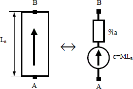
Using the Amperian current model of the magnet and if we neglect the fictitious currents inside the magnet ![]() and the flux leakages in the magnet, the equivalent circuit of a rigid magnet consists of a magnetomotive force ε in series with magnet reluctance ℜa (Figure 1.15). With:
and the flux leakages in the magnet, the equivalent circuit of a rigid magnet consists of a magnetomotive force ε in series with magnet reluctance ℜa (Figure 1.15). With:
![]()
Figure 1.15. Equivalent circuit of a magnet
For example, the circuit presented in Figure 1.14a can be replaced by the equivalent circuit given by Figure 1.16.
Figure 1.16. Equivalent circuit of a magnetic circuit excited by a magnet

Re and Rf are respectively the reluctances of the air-gap and iron. The magnetic flux Φ is then given by:
![]()
1.3.3. Inductances
Electrical circuits are supposed to be in free space.
1.3.3.1. Mutual inductances
Let's consider two circuits (C1) and (C2) having respectively N1 and N2 turns (Figure 1.17). Only (C1) is supposed to be supplied by current I1.
Figure 1.17. Electrical circuits (C1) and (C2)

The total flux in (C2) created by I1 is given by:
![]()
M12 is the mutual inductance between (C1) and (C2). With:
[1.26] ![]()
M12 is therefore proportional to the product N1N2. In the same way, if only (C2) was supplied by I2, the total flux in (C1) would be:
![]()
with:
![]()
1.3.3.2. Self-inductances
Self-inductance M11 = L1 would be obtained by the previous test if C1 and C2 were joined. Expression [1.26] cannot be used because of indetermination when r tends to zero. It is thus preferable to determine L1 from the associated energy. However when the flux flows in a magnetic circuit surrounded by a coil (i.e. case of a winding or a transformer), it can be calculated in restricting the surface to that of the magnetic circuit not including the coil:
![]()
If the circuit consists of N1 turns, the total flux is:
![]()
The self-inductance is then obtained by:
[1.27] ![]()
Flux ϕ1 being proportional to N1, it can be noticed that L1 is proportional to (N1)2.
1.3.3.3. Coupled circuits
Let us consider two circuits (C1) and (C2) from Figure 1.17 again, and let us suppose that they are respectively supplied by currents I1 and I2. The total flux created by I1 equals L1I1. A part of this flux, equal to M12I1, crosses circuit (C2). The total flux crossed by (C1) and (C2) is therefore given by:
![]()
with M12 = M21 = M:
![]()
It is then written in a matricial form:
![]()
The co-energy (numerically equal to the energy in a linear case) associated with those two circuits is given by:
![]()
and thus:
![]()
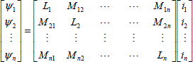
This result can be generalized to n coupled circuits:

[1.28] ![]()
[I]t = [I1 I2 … In] being the transpose of matrix [I].
1.3.3.4. Inductances, reluctances, permeances
A magnetic circuit of reluctance ℜ, crossed by magnetic flux ϕ (Figure 1.18) is considered.
Figure 1.18. Magnetic circuit of reluctance ℜ

We have Ni = ℜ ϕ, where:
– ϕ is the flux embraced by one turn of the coil.
– The total flux in the coil is ψT = N ϕ.
– ψT is related to current I by self-inductance L: ψT = L i. thus, N ϕ = L i = N2 i/ℜ.
The self-inductance of a coil is therefore bound to reluctance ℜ (or to permeance ℘) of the corresponding magnetic circuit by:
[1.29] ![]()
This shows that the self-inductance of a coil is forwardly related to the permeance of its magnetic circuit. This is also the case for the mutual inductances between two coils.
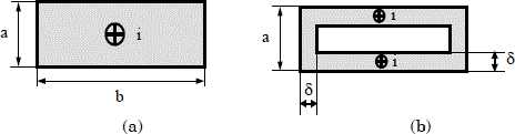
1.3.4. Skin effect or Kelvin effect
Let us consider one homogenous conductor with a rectangular cross-section S characterized by permeability μ and conductivity σ, and travelling by current i (Figure 1.19). When i is DC, current density J is constant in the entire cross-section S. J is not constant for an alternating current.
In this case, the field leads to auto-induction phenomena and there is a current concentration on the surface which is all the more important when the frequency is high. The conductor then has a higher electrical resistance than the resistance obtained with forward current; it is sometimes necessary to subdivide the conductors, particularly when frequency increases.
Skin thickness δ is defined as being the thickness of the layer in which most of the current is concentrated.
[1.30] ![]()
As an example, for copper, δ approximately equals 1 cm at 50 Hz, and 2 mm at 1 kHz.
Figure 1.19. Schematic representation of the current repartition in a conductor: a) forward current; b) alternating current
1.3.5. Torque calculation using the virtual work principle
1.3.5.1. Single-phase system
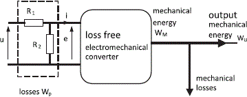
Let us consider a single-phase system (Figure 1.20) converting electrical energy into mechanical energy. Electrical energy W1 provided by the source is the sum of energy Wp dissipated in losses, of energy Wem stored in the electromagnetic field and of converted mechanical energy WM.
Figure 1.20. Energy balance in electromechanical energy conversion

Losses Wp do not affect the conversion process. The diagram of Figure 1.21 in which losses Wp are dissipated in equivalent resistances R1 and R2 is adopted. The system is supplied by voltage u and the loss free converter absorbs current i. The energy supplied to the idealized converter can then be expressed in terms of the electromotive force e:
![]()
It can also be written in a differential way:

Figure 1.21. Loss free converter
Considering a rotating converter, the mechanical energy generated during time dt is linked to the electromagnetic torque Γe by:
![]()
For a system in translation in direction x, this energy is related to force F by:
![]()
In the following we shall consider that the system is rotating:
![]()
This equation shows that energy Wem is a function of flux ψ and of position θ. It can then be written:
![]()
then:
![]()
It is important to note that the electromagnetic torque is obtained by deriving Wem in terms of position θ, while keeping a constant flux. This constraint is not easy to achieve. Co-energy d ![]() em is introduced by:
em is introduced by:
![]()
thus:
![]()
then:
![]()
The electromagnetic torque therefore equals the derivative, with constant current, of the co-energy in terms of position θ.
1.3.5.2. Generalization: polyphase systems
Let us consider a multiphase system absorbing currents i1, i2… in with respective voltages v1, v2… vn. If dWp is the sum of the electrical losses before the electromagnetic transformation, we get:
![]()
with:
![]()
Since:
![]()
we get:
[1.31] ![]()
As the state variables are flux ψ and position θ:
![]()
thus:
[1.32] ![]()
[1.33] ![]()
In the same way, co-energy ![]() is introduced by:
is introduced by:
![]()
thus:
![]()
The state variables are currents ij and position θ, then:
![]()
It can be deduced that:
[1.34] 
[1.35] ![]()
1.3.5.3. Linear systems
Fluxes and currents are linked by a linear law. Energy and co-energy are then numerically equal.
1.3.5.3.1. Single-phase systems
We have:
![]()
L is the self-inductance of the phase with n turns, and ℜ is the reluctance of the corresponding magnetic circuit. L and ℜ can depend upon position θ. With a fixed θ, energy is given by:
![]()
ϕ is the flux per turn with ψ = nϕ.
In the same way, co-energy is given by:
![]()
The electromagnetic torque can therefore be calculated indiscriminately by:
![]()
or by:
![]()
1.3.5.3.2. Polyphase systems
Fluxes and currents are related by:
Co-energy is given by:
![]()
which can be written:
![]()
In the same way, energy is expressed:
![]()
The electromagnetic torque can therefore be obtained indiscriminately by:
[1.36] ![]()
or by:
[1.37] ![]()
1.4. Power electronics
Since the 1960s, power electronics have made considerable modifications in electrical engineering and particularly in the implementation of electrical machines. Thanks to the development in semi-conductors, motors are mainly supplied by static converters. That is why it is useful to mention in the present chapter the functioning principles and the main characteristics of static converters associated with electrical machines. For simplification we shall restrict the presentation to idealized functioning of the most common converters.
Power electronics are in constant and quick technological evolution, particularly regarding components technology. In order to make writing easy we shall assume that “traditional” components are used: diodes (represented by D) or thyristors (represented by T) for rectifiers or naturally commuted inverters, thyristors for AC power controllers. Concerning choppers and inverters, we shall consider that fully controlled switches (bipolar or field effect transistors, GTO, IGBT, etc.) denoted Tc are used. This does not alter the validity of the results presented in the following.
1.4.1. Rectifiers and naturally commutated inverters
1.4.1.1. Introduction
Rectifiers ensure an AC-DC energy conversion. They are constituted of diodes (in that case the output voltage is constant in average value) or of thyristors in order to make the output voltage variable or regulated.
1.4.1.2. 3-phase bridge converters
3-phase bridge rectifiers are largely used for the control of electrical machines. Figure 1.22 represents a thyristor-based 3-phase bridge. The time variation of the output voltage is shown in Figure 1.23a and the currents absorbed from the AC supply are represented on Figure 1.23b. Assuming the bridge conduction to be uninterrupted and neglecting the commutation phenomena, the average value of the rectified voltage is:
[1.38] ![]()
where V is the rms value of the phase voltage of the source, and α, the firing angle of the thyristors.
Figure 1.22. Thyristor bridge
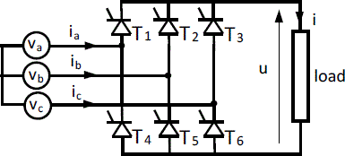
Figure 1.23. Load voltage (a) and source phase current (b) of a 3-phase thyristor bridge. ib and ic are shifted by ± 2 π /3 with respect to ia

1.4.1.2.1. Single-phase bridge
When a 3-phase source is not available, a single-phase bridge is used (Figure 1.24). With the same assumptions, the mean value of its output voltage is:
[1.39] 
Figure 1.24. Single-phase bridge

1.4.1.2.2. Diode bridge
A diode bridge can be considered to be a thyristor bridge with a zero firing angle. The mean value of its output voltage will then be respectively ![]() and
and ![]() for 3-phase and single-phase bridges.
for 3-phase and single-phase bridges.
1.4.1.3. Inverter mode
Equation [1.38] shows that if α is greater than π/2, U0 becomes negative. The output current of the bridge, I0 (considered as constant in a first approximation) remains positive, the AC to DC power flow becomes negative and the bridge works as an inverter. The DC “load”, of course, has to be active in order to become a generator. The DC voltage is then as shown in Figure 1.25.
The inverter mode of thyristor bridges also requires that the AC system has electromotive forces in order to ensure the commutation of the thyristors.
1.4.1.3.1. Maximum firing angle
In order to take into account the components blocking conditions, it is necessary that α < π, and,to take the various commutation and overlap phenomena into account, the value of the firing angle is limited to π – β,where β is a guarding angle often called “minimum extinction angle”.
Figure 1.25. Output voltage of a thyristor bridge (inverter mode)

1.4.1.3.2. Reversibility
The transition of the thyristor bridge from “rectifier” mode to “inverter” mode allows us to reverse the direction of the energy transfer. However, this reversibility is only partial because only the voltage changes sign; the current remaining positive. In order to reverse the current in the AC side it is necessary to use two thyristor bridges anti-parallel connected (Figure 1.26), giving a four-quadrant converter.
Figure 1.26. Four-quadrant AC-DC converter

1.4.2. AC thyristor controllers
1.4.2.1. Single-phase AC controller
A single-phase AC controller is generally constituted of two anti-parallel connected thyristors. It ensures power transfer from an AC voltage source to an AC load (Figure 1.27).
Thyristors are usually controlled with a firing angle ψ the origin of which is the zero crossing of the source voltage (Figure 1.28).
Figure 1.27. Single-phase AC controller

Depending on the nature of the load, voltages and currents represented in Figure 1.28 are obtained.
Figure 1.28. Load voltages and currents. Single-phase AC controller: a) resistance load b) and c) resistance and inductive load (ψ > φ), where the current is out of phase by φ with respect to the voltage


When ψ varies, rms value Veff of the load voltage varies; however, the relation between ψ and Veff is not simple. For example, on the resistance load:
[1.40] ![]()
If the load is inductive, the calculation of Veff depends on the load parameters and is complicated, but Veff remains a decreasing function of ψ. Furthermore the load voltage and, consequently, the current have important harmonic components.
1.4.2.2. 3-phase AC controllers
The most common structure (fully controlled star connected load) of an AC controller designed for power supply or motors is represented in Figure 1.29. As there is no connection between the source and the load neutrals there is no circulation of 3k rank harmonics which would give zero sequence currents in the machines.
Figure 1.29. 3-phase AC controller

This converter allows us to supply a 3-phase load by a non-sinusoidal voltages constant frequency and which rms value is controlled by the firing angle ψ. As for the single-phase AC controller, the load voltages (and therefore the currents) have a high harmonic content.
1.4.3. Choppers
Choppers ensure energy transfer between two DC systems with different voltages.
1.4.3.1. Step-down chopper
The diagram of the basic step-down chopper is represented in Figure 1.30. Its functioning assumes that the source is a “voltage” source (voltage E is a state variable and cannot have any discontinuity) and that the load is a “current type” receiver, the presence of an inductance preventing current discontinuities.
Assuming that Tc is switched on with a period T and switched off after a delay αT(α ∈ [0,1]), the voltage and the current waveforms of Figure 1.31 are obtained. The average value of the load voltage is therefore αE, from which we derive the name “step-down DC to DC converter”. The average output DC voltage is adjusted using the variation of α.
Figure 1.30. Step-down DC to DC converter

1.4.3.2. Boost chopper
In order to ensure energy transfer between a source with a voltage E and a load of voltage E' (with E' > E), the circuit represented in Figure 1.32 can be used. This matches the previous circuit. The structure including a step-down chopper and a boost chopper (regenerative chopper) enables a bi-directional energy transfer between a DC source and a DC load.
Figure 1.31. Voltage (a) and load current (b) of a step-down DC to DC converter

Figure 1.32. Boost chopper

1.4.4. Cycloconverters
These are AC-AC converters enabling forward variation of the load currents frequency. They are rarely used and only for very high power applications. Interest in cycloconverters is decreasing.
1.4.5. Force commutated inverters
These converters ensure energy transfer from a DC source to an AC load (single-phase or 3-phase). They are based on the use of fully controlled switches. The elementary structure includes a fully controlled switch (transistor, GTO, IGBT, etc.) connected in an anti-parallel with a diode. The set of two elementary structures connected to a same phase of the load makes an “inverter leg”.
A force commutated 3-phase inverter is generally constituted of three inverter legs, one per phase (Figure 1.33).
Figure 1.33. Force commutated 3-phase inverter

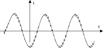
When controlled by pulse width modulation (PWM), force commutated inverters provide load currents with few harmonics (Figure 1.34). The fundamental frequency of voltages and currents imposed by the switch control can vary over a wide range. Force commutated inverters are therefore very useful for obtaining almost sinusoidal 3-phase systems with variable frequencies.
Figure 1.34. Current in a load supplied by a PWM inverter