Chapter 1

The economy's production possibilities curve is shown by the solid line in the figure accompanying these answers.

1. Twelve million units of capital goods (capital goods decreased from 32 to 20 million units); 10 million units of consumer goods (consumer goods decreased from 10 million units to zero).
2. Point A is slightly to the left of the production possibilities curve, and point B is further to the left than point A.
3. The location of point C depends on how one views the relative importance of capital goods and consumer goods. Point C will be closer to the horizontal axis if capital goods are considered to be relatively more important, and closer to the vertical axis if consumer goods are considered to be relatively more important. Students put point C on the curve based on their opinions about the relative importance of capital goods and consumer goods.
4. If only consumer goods were produced, no machinery or equipment would be produced to replace what is currently being used, and future production would be adversely affected. If only capital goods were produced, there would be nothing to sustain people currently.
5. The production possibilities curve would shift to the right as illustrated by the lighter line in the accompanying figure.

   

Chapter 2

1. 1. pure market
   2. pure planned
   3. mixed
   4. pure market
   5. pure planned
   6. mixed
2. 1. Flow of money from households to businesses and flow of goods and services from businesses to households; saving more and spending less reduces the money flow and the goods and services flow.
   2. Flow of factors of production from households to businesses and flow of income from businesses to households; reducing the flows on the bottom half reduces the flows on the top half.
   3. Saving more and spending less decreases the production of goods and services which, in turn, decreases employment of resources and income.

Chapter 3

1. d; supply curve shifts to the left; increase; decrease
2. a; decrease demand curve shifts to the right; increase; increase
3. d; supply curve shifts to the left; increase; decrease
4. e; no shifts; none; none (changes price, not a nonprice factor)
5. b; demand curve shifts to the left; decrease; decrease
6. a; demand curve shifts to the right; increase; increase
7. c; supply curve shifts to the right; decrease; increase
8. b; demand curve shifts to the left; decrease; decrease
9. a; demand curve shifts to the right; increase; increase
10. e; no shifts; none; none (changes price, not a nonprice factor)
11. b; demand curve shifts to the left; decrease; decrease
12. c; supply curve shifts to the right; decrease; increase
13. e; no shifts; none; none (changes price, not a nonprice factor)
14. c; supply curve shifts to the right; decrease; increase

Chapter 4

1. Price Index	Price Index
   80.0	64.0
   100.0	80.0
   110.0	88.0
   125.0	100.0
   130.0	104.0
   150.0	120.0

2. 
3. Real GDP 2006: $1,000; 2007: $1,000; 2008: $1,200; 2009: $1,250; 2010: $1,250; 2011: $1,200; 2012: $1,250
   1. The economy's output did not grow from 2006 to 2007, grew from 2007 through 2009, did not grow in 2010, decreased in 2011, and grew again in 2012.
   2. Unlike the impression given by money GDP, the economy's real GDP, or output, did not grow every year, and in 2011 it actually declined. Also, the overall growth rate in output from 2006 through 2012 was not nearly as great as money GDP would lead one to believe.

Chapter 5

From each action taken alone, output and employment would change as follows:

1. increase
2. decrease
3. increase
4. increase
5. decrease
6. no change (demand-pull inflation would result)
7. decrease
8. increase
9. increase
10. no change (demand-pull inflation would result)
11. decrease
12. decrease
13. no change (demand-pull inflation would result)
14. increase
15. decrease

    From each of these actions, total output and income would change as follows:

16. increase by $200 million
17. decrease by $87.5 billion
18. increase by $400 million
19. decrease by $12 billion
20. decrease by $12.5 million ($20 million export injection − $25 million import leakage ÷ 40.40 = −$12.5 million)
21. increase by $400 million (80 percent of $100 million transfer payment = $80 million in spending; $80 million ÷ 0.20 = $400 million)

Chapter 6

1. output and employment increase
2. output and employment will decrease (some portion of the Social Security will be saved and not spent while all of the government purchases amount will be a decrease in spending)
3. price levels increase
4. output and employment increase
5. output and employment decrease
6. output and employment decrease
7. output and employment decrease
8. output and employment increase
9. price levels increase
10. price levels increase
11. output and employment decrease
12. output and employment decrease
13. output and employment increase
14. output and employment decrease

Chapter 7

1. $18,871,340
2. $38,014,440
3. $11,956,741
4. $14,840,000

Chapter 8

1. required reserves = $1,350,000; actual reserves = $6,000,000; excess reserves = $4,650,000
2. new loans = $9,700,000
3. new borrowing = $50,000
4. money multiplier = 12.5;

   money supply increase = $625,000,000

5. decrease in excess reserves = $335,000
6. new excess reserves = $2,000,000
7. new excess reserves by Carolina Coast = $0;

   new excess reserves by Inland Bank = $4,000,000

8. money supply increase = $280,000,000

Chapter 9

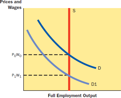
1. Draw a vertical supply curve (S) at full employment output and a downward sloping demand curve (D). a. Label their intersection as P₀W₀. b. Draw a demand curve (D1) that has shifted to the right. c. Label the intersection of D1 and S as P₁W₁. d. The economy arrived at this new position because prices and wages are flexible downward. See the following graph.

   

2. Total Output	Economic Condition
   $0	Expansion
   $200	Expansion
   $400	Expansion
   $600	Equilibrium
   $800	Contraction
   $1,000	Contraction

   

3. 
   1. In the short run, a decrease in demand would bring a slight decrease in prices and a decrease in output. In the long run, a decrease in demand brings a decrease in prices but no change in output.

Chapter 10

1. increase in supply causing equilibrium price to fall
2. increase in demand and a possible decrease in supply causing equilibrium price to rise
3. decrease in demand and a possible increase in supply causing equilibrium price to fall
4. decrease in demand and increase in supply causing equilibrium price to fall
5. increase in supply causing equilibrium price to fall
6. decrease in demand and increase in supply causing equilibrium price to fall
7. increase in demand causing equilibrium price to rise

Chapter 11

According to Table 1, Pete should charge $98 and complete 4 drawings to maximize his profit from the drawings. In going for volume, as suggested by his roommate, his total profit would be $128 less than that received from producing and selling 4 drawings.

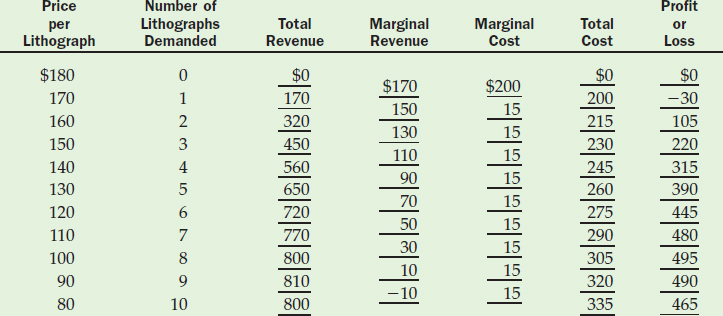
As for the lithographs, Pete should charge $100 each and sell 8, earning a total profit of $495. This is indicated in Table 2.

TABLE 1 Custom-Drawn Houses

TABLE 2 Lithographs

Chapter 12

1. 92%, fall, lower, 85.5%

   fall, lower, 83.7%

   rise, higher, 86%

2. 
3. $2,025; $3,042; $6,183; $2.25; $1.90; $2.29
4. 

Chapter 13

1. The total revenue values in the table are: $0, $2, $4, $2,000, $2,002, $2,004, $20,000, $20,002, $20,004. All marginal revenue values are $2.00.
   1. Draw a perfectly horizontal line at $2.00 and mark it D = MR
   2. 7,000 bushels
   3. $2.50; loss $0.50; loss $3,500
   4. Draw a perfectly horizontal line at $3.50 and mark it D = MR
   5. 9,000 bushels
   6. $2.50; profit $1.00; profit $9,000
2. 5,000 units; $9.00; $5.00; profit $4.00; profit $20,000

Chapter 14

1. social regulation—Environmental Protection Agency
2. no government intervention
3. social regulation—Consumer Product Safety Commission
4. antitrust enforcement—Sherman Act Section 1 price fixing violation
5. no government intervention—the sellers are pure competitors responding to the price rather than fixing it
6. industry regulation
7. antitrust enforcement—Celler-Kefauver Act
8. no government intervention
9. industry regulation
10. antitrust enforcement—Sherman Act Section 2 monopolization violation

Chapter 15

In Table 1, marginal product is 500, 500, 500, 400, 300.

1. the fourth worker

   In Table 3, total revenue is $0, $25, $45, $60, $66.50, $67.50. Marginal revenue product is $25, $20, $15, $6.50, $1.00.

2. $25 per hour
3. $15 per hour
4. no, the MRP of the fifth worker is just $1

In Table 4, the quantity of workers demanded with each wage rate is 1—$25; 2—$20; 3—$15; 4—$6.50; 5—$1.00. These numbers are used to plot the demand curve in the figure.

Chapter 16

1. 1. 1/2, 2, Canada
   2. 2, 1/2, Brazil
   3. 12, 12
   4. 16 of wheat, 16 of soybeans
   5. 8, 8
2. 1. 1/5, 4, Mexico
   2. 5, 1/4, Venezuela
   3. 525, 200
   4. 1,000 lamps, 200 gallons of gasoline
   5. 50, 200

Chapter 17

1. decrease, decrease, decrease, increase
2. increase, decrease, increase, increase
3. increase, increase, increase, decrease
4. decrease, increase, decrease, decrease
5. increase, increase, increase, decrease
6. decrease, increase, decrease, decrease or increase depending on whether the effect of the change in demand was greater or less than the effect of the change in supply, increase