
Energy harvesting for infrastructure sensing systems
J.T. Scruggs, University of Michigan, USA
Abstract:
This chapter gives an overview of some of the fundamental design issues arising in vibration energy harvesting systems for sensing applications. We focus primarily on piezoelectric and electromagnetic transducers. Linear dynamical models for these systems are presented and discussed. Impedance matching theory is discussed, and its application to monochromatic energy harvesting is explained. Fundamental limits on power generation are presented for monochromatic disturbances, and analogous limits for stochastic disturbances are briefly presented. Passive tuning techniques are discussed, for reactive power compensation.
A number of basic electronic circuits for extracting power from harvesters are described, including the standard diode bridge rectifier, DC/DC converters, and synchronized switch harvesting inductor (SSHI) circuits. Applicability and tradeoffs between these circuits are discussed. The article closes with some comments about current research trends in small-scale vibration energy harvesting.
Key words
vibration; energy harvesting; impedance matching; power electronics
18.1 Introduction
In many wireless sensing applications, power availability issues pose some of the most daunting challenges. These sensors are intended for use over the service life of a structure, which implies decades of operation. On-board battery storage systems present obstacles toward the achievement of this objective for a few reasons. In general, they must be periodically replaced or recharged as their energy is depleted. This requirement of routine maintenance may be undesirable in many applications. For example, it limits usage of the sensor to applications in which the unit (or at least its energy storage subsystem) can be easily accessed. This prohibits such sensors from being truly embedded in smart structures, and also may prohibit their reliable use in remote and hostile environments. Moreover, it is a well-known fact that the energy and power density of power storage technology has grown at a much slower rate than the energy and power requirements of small-scale intelligent systems.1 These issues have motivated a considerable amount of research activity over the last decade, toward the development of autonomous technologies to harvest energy for wireless sensors, from physical phenomena in proximity to the sensor.
There are indeed a variety of localized energy sources that may be tapped to power wireless sensors. In applications where sensors are mounted to the exterior of a structure, or where they are exposed to ambient lighting, solar energy collection is arguably the most straightforward technology. Integration of small solar panels into wireless sensing units has been demonstrated, and such systems are actually available commercially. Energy may also be harvested from temperature differentials, through a variety of thermal power conversion techniques. In applications where significant fluid flows exist, microturbines can be used to convert this flow energy into electricity, or it can be extracted from deliberately induced turbulence, through a variety of means. In other applications in which a structure or material is subjected to slowly varying (i.e., quasi-static) stresses, piezoelectric materials can be used to harvest a resultant strain-induced charge. Furthermore, there are also opportunities in many applications to wirelessly transmit radio frequency (RF) energy.
All the above techniques, and especially solar energy systems, have been widely explored in the context of wireless sensing nodes. The recent survey by Sudevalayam and Kulkarni2 provides an excellent recent snapshot of where these technologies are, both in terms of the vanguard of research and development, as well as for readily available commercial units. For solar energy harvesting in particular, a number of plug-and-play devices and development boards can now be purchased for wireless sensor applications, including products from Texas Instruments, Cymbet Corporation, MicroStrain, EnOcean, Solarcraft, Midé, and several others.
It is often argued that for many structural systems, the most pervasive type of energy available to embedded and inaccessible sensors is low-level vibratory energy. This energy manifests itself in the form of machinery vibrations, vehicular traffic, pedestrian activity, etc. Because of the ubiquity of the resource, vibratory energy harvesting (VEH) technology has been the subject of considerable research, with applications spanning the fields of civil, aerospace, transportation, and biomedical engineering. Also for this reason, VEH systems are the focus of this chapter. Many surveys have been written recently, which give snapshots of the status of the technology in this field.3–8 It is not the purpose of this chapter to provide such a survey, which would inevitably become out-of-date after a short time. Instead, this chapter will concentrate on establishing the theoretical basis for VEH systems, and will illustrate how their technological particulars translate into fundamental engineering problems.
In order to harvest vibratory energy, it must be converted to electricity via some mode of transduction. Typically this transduction is embedded in a resonant electromechanical system that we will call the harvester, which is mounted on a larger vibrating structure. The larger structure is assumed to be massive in comparison to the harvester, such that its acceleration can be assumed to be unaffected by the dynamic behavior of the harvester. (This assumption is not necessary in order to analyze and design energy harvesters, but it does simplify the analysis and is valid in many applications.) A harvester is typically tuned such that its natural frequency is within the disturbance passband. At the μ W-mW scale, there are three general modes of transduction that have historically been dominant in applications: electro-magnetic, piezoelectric, and electrostatic transduction.
Electromagnetic transducers are typically coupled to a single degree-of-freedom (SDOF) sprung mass, as shown in Fig. 18.1a. The transducer simply comprises a moving magnet in a coil, as shown. Speaking broadly, one of the challenges posed by this type of transduction is that it is generally difficult to generate useful voltage levels as the scale becomes small. This is because an electromagnet generates a voltage in proportion to its velocity, with the constant of proportionality growing with the strength of the magnet and the number of coil windings. It is therefore quite difficult to design electro-magnetic harvesters with acceptable voltage levels, as the size requirements become more restrictive. However, a number of researchers have demonstrated impressive small-scale prototypes.9
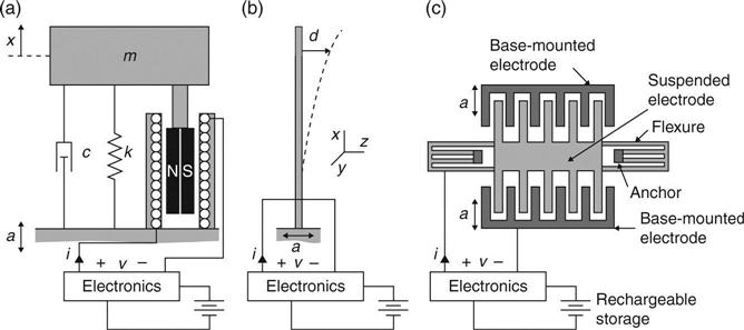
Piezoelectric transduction can be embedded into several different types of resonant harvesters, but one of the more common approaches is to bond a layer of piezoceramic material (such as lead zirconate titanate, or PZT) to a flexible beam, which is mounted on the vibratory surface as shown in Fig. 18.1b. This particular configuration is called a bimorph configuration, because the material is bonded to both sides of the beam, with the top and bottom electrodes connected, either in series or parallel. Piezoelectric transducers are arguably the most prevalent at small scale, and have been implemented by many researchers.4,6 When properly designed, they are capable of generating useful voltages even when strains are very small, and they are easier to fabricate at small scale than electromagnetic transducers. However, as we will discuss in Section 18.4, these advantages do come at a price, in the form of more complicated power processing circuitry.
For applications at the micro-electromechanical systems (MEMS) scale, electrostatic transducers may be a more viable transduction mode. These devices, illustrated in Fig. 18.1c, consist of comb-shaped electrodes, connected through a flexible linkage. The outer electrode is mounted to a base, while the central electrode remains suspended. When the base is shaken, this causes the suspended electrode to resonate, thus causing its teeth to oscillate in and out of those of the base electrode. This has the effect of varying the capacitance between the two electrodes. If the voltage between the electrodes is controlled in coordination with these oscillations in capacitance, this results in energy conversion. Electrostatic harvesters have been successfully demonstrated for use in MEMS systems.10,11 Although they do scale down very well for MEMS integration, they also require the most sophisticated electronics of the three transduction modes discussed.12 Additionally, we note that piezoelectric transduction has also been successfully implemented at MEMS scales.13
In this chapter, we will focus on electromagnetic and piezoelectric harvesters, which can be analyzed using similar techniques, and which have been demonstrated to be viable sources of power for a multitude of sensor applications.
A number of VEH systems are commercially available, although it must be said that at the present time most products operate at vibration power levels and base acceleration levels that are far in excess of what is typical for sensing applications in civil engineering. A few of the VEH modules currently available off-the-shelf (i.e., as a system, including the transducer, power electronics, and in some cases, local storage) are given in Table 18.1. Many of these products were originally developed for applications with strong vibratory signatures, such as machine and heating, ventilation and air conditioning (HVAC) monitoring, as well as aerospace and defense applications. Some of these companies (such as Midé) have demonstrated their devices to be scalable well below their ratings. Beyond the companies listed in this table, several more (such as Smart Material, PowerCast) offer customizable energy harvesting evaluation kits, which provide modular components for power conversion and storage, but which also allow for considerable customization. Many other companies, (such as MicroStrain and Ambio Systems, to name just a few), provide wireless sensing motes that afford plug-and-play compatability with VEH transducers.
Table 18.1
A sampling of commercially available VEH systems
| Model | Company | Type | Weight | Rating |
| VEH 460 | Ferro solutions | EM | 0.43 kg | 0.3 mW at 25 mg, 60 Hz |
| PMG FSH | Perpetuum | EM | 1.075 kg | 0.43 mW at 25 mg, tunable frequency |
| MVEH | MicroStrain | EM | 216 g | 4 mW at 0.2 g, 20 Hz |
| PVEH | MicroStrain | PE | 185 g | 30 mW at 1.5 g, 1 kHz |
| Volture | Midé | PE | – | 1.45 mW at 1 g, 120 Hz, no tip mass |
| 9.2 mW at 1 g, 40 Hz, 15.6 g tip mass | ||||
| Harvestor | Advanced Cerametrics |
PE | – | 0.4 mW at 3 g, 30 Hz 0.81 mW at 3 g, 220 Hz |
| VH-1 | KCF | PE | 134 g | > 0.7 g, no power/frequency rating |

Techniques to scale the technology down have been demonstrated in the literature (see, e.g., References 13 and 14), but at present these have not fully crossed the threshold into wide availability, commercially. As such, applications with smaller power scales presently require at least some custom design. Scaling the technology down to lower power levels constitutes a significant challenge, especially in regards to the electronics design. We will touch on some of these challenges later in the chapter.
18.2 Harvester dynamic modeling
In this section we present the basic dynamic models for electromagnetic and piezoelectric harvesters, followed by a system-theoretic discussion of more general properties common to the dynamic models of many energy harvesting technologies.
18.2.1 Electromagnetic transducers
Harvesters with electromagnetic transduction, such as the one in Fig. 18.1a, convert power via Faraday’s law, by the equations
[18.1]
where Ke is an electromagnetic conversion constant that is a function of the geometry of the coil, number of turns, and the magnetic field of the magnets. The specific functional dependency of Ke is typically linear in the field intensity and number of turns, while the dependency on the geometry depends on the configuration of the coil relative to the magnets.11,15 The expressions in Equation [18.1] constitute the linearized version of what is always, to one degree or another, a nonlinear phenomenon exhibiting hysteretic and other losses.
The harvester dynamics are governed by the standard second-order differential equation
[18.2]
In the Laplace domain, voltage v is a consequence of dynamic system inputs a and i, as
[18.3]
where
[18.4]
[18.5]
18.2.2 Piezoelectric transducers
We assume a composite beam such as the one shown in Fig. 18.1b, in which piezoelectric material is bonded to a substrate material (such as aluminum). It is not necessarily the case that the cross-sectional properties of the beam are constant; indeed, there is some benefit to making the beam become progressively more slender as it extends from the root, as this makes strain deformations more uniform in the fundamental mode. It is also not necessarily optimal to bond the transducer patch over the entire extent of the beam, as is depicted in the figure. Rather, in many designs the patch extends from the root only a fraction of the beam length. This is advantageous because by placing the transducer only where the strain is high, the voltages produced can be higher. Finally, it is often the case that a proof mass is attached to the end of the beam. This can be used to tune the resonant frequency of the beam, as well as having other advantages.
In Reference 16, the electromechanical dynamics of a beam with multiple bimorph piezoelectric transducers were derived. Here, we merely provide an overview, specializing to the single-transducer case. Let ρ(x, y, z, t ) denote the density at location {x, y, z} in the substrate–piezo composite. Let S(x, y, z, t) ∈ ℜ6 and T(x, y, z, t) ∈ ℜ6 denote the Voigt (i.e., vector) form of the strain and stress tensors, and let E(x, y, z, t) ∈ ℜ3 and D(x, y, z, t) ∈ ℜ3 denote the electric field and displacement vectors. Then for small deformations and small fields, we can assume the linear, coupled constitutive law relating {S, E} to {T,D}, i.e.,
[18.6]
where c is the modulus of elasticity at zero field, ε is the dielectric constant matrix at zero strain, and e is the coupling coefficient matrix. (Note that in the substrate material, e and ε are zero.)
Assuming the classical Bernoulli-Euler assumptions for the beam deformation, define d(x, t) as the transverse deflection of the beam centroid, and then it follows that
[18.7]
A standard Galerkin approximation is typically used for d(x, t), i.e.,
[18.8]
where r(t) is the vector of generalized displacements, and ϕ(x) is the vector of Galerkin shape functions for each generalized displacement. Electric field E is assumed to be constant inside each patch, zero in the substrate, and oriented in the êy direction everywhere; i.e.,
[18.9]
where êy is the unit vector on the y direction, ψ(y) is a function of the patch thickness and beam geometry.
With these assumptions, the differential equations for the reduced-order system are found as
[18.10]
[18.11]
where {M, K, Θ, G, Cp} are found through the standard Rayleigh-Ritz projection. These terms are, respectively, the generalized mass and stiffness matrices, the coupling factor matrix, disturbance input matrix, and piezoca-pacitance. Generally, mechanical damping matrix C is found after the fact e.g., through a Rayleigh damping assumption. The dielectric leakage resistance Rp , is extremely high for typical designs, and is often assumed to be infinite.
As with the case of the electromagnetic harvester, the Laplace domain characterization of the above is
[18.12]
but where in this example the above transfer functions are
[18.13]
 [18.13]
[18.14]
 [18.14]
18.2.3 General properties
Transfer function Gi(s) is the input impedance of the transducer. One can think of it as the driving-point impedance of an electric circuit that is equivalent to the true system from the vantage point of the harvesting electronics. Because harvesters are passive systems (i.e., they typically have no internal energy sources), this equivalent network will also be passive, i.e., it can be built from ideal resistors, inductors, capacitors, transformers, and gyrators. Because of this, one can always assume that Gi(s) is positive real, i.e.,
[18.15]
This property turns out to be important, in the determination of the maximum power generation for energy harvesters.
18.3 Power availability and the optimal harvesting admittance
This section is concerned with the determination of how much power one can expect to generate from a given disturbance, using a given harvester. Specifically, we derive upper limits on the available power, by assuming the electronics are very efficient. This assumption is never completely justifiable, and invariably gives overly optimistic estimates of available power. On the other hand, the analysis is still useful because if the power levels derived here are insufficient for a given application, it can be determined immediately that there is no hope of a given disturbance/harvester combination meeting a design specification. We will keep the discussion general to all linear harvesters, although the results here do specialize on many of the more specific cases derived in the literature (such as in Reference 17 for piezoelectric devices).
18.3.1 Classical impedance matching theory
Consider the case in which a(t) is a finite-energy signal, i.e., one for which ∫ 0∞a2(t)dt is finite, and let â(s) be its Laplace transform. Similarly, let ![]() and
and ![]() be the Laplace transforms for the corresponding current and voltage, which we also assume to have finite signal energy. The total amount of energy absorbed from the transducer by the electronics is
be the Laplace transforms for the corresponding current and voltage, which we also assume to have finite signal energy. The total amount of energy absorbed from the transducer by the electronics is
[18.16]
By the Plancharel theorem, we have that this energy is equivalent to
[18.17]
Substituting Equation [18.12], we have
[18.18]
Now, consider that at each ω we can find the ![]() maximizing Eabs. Performing this maximization, with the constraint that
maximizing Eabs. Performing this maximization, with the constraint that ![]() is the complex conjugate of
is the complex conjugate of ![]() , gives the optimal current as
, gives the optimal current as
[18.19]
Correspondingly, the voltage ![]() with the optimal
with the optimal ![]() imposed, is
imposed, is
[18.20]
and the optimized absorbed energy is
[18.21]
Recognizing that Im{Gi(jω)} = − Im{Gi(− jω)}and Re{Gi(jω)} = Re{Gi(− jω)} the above is equivalent to
[18.22]
Note that the integrand above is real and positive at all frequencies, and constitutes the spectrum of optimized energy.
In the Laplace domain, the optimal ![]() may be expressed as a feedback function of
may be expressed as a feedback function of ![]() as
as
[18.23]
where
[18.24]
is called the impedance matched feedback law. However, unlike our usual conventions for feedback, Y(s) above would need to be anticausal (i.e., anticipatory) in order for the closed-loop system to be stable. (In the time domain, this fact would be evident from the impulse response of Y(s) being left-handed, rather than right-handed.) As such, we can say that in general, in order for an VEH system to maximize the physically-available power, it must make power generation decisions based on future disturbance information.
18.3.2 Power availability and tuning for monochromatic disturbances
Now, consider the case in which a(t) is monochromatic, i.e.,
[18.25]
for time-invariant a0 and ω0. In this case, it turns out that an analogous optimization can be done, again arriving at the same matching condition in Equation [18.24]. However, in this case, â(jω) is zero at all frequencies except ω = ω0, and it is therefore only necessary for a feedback law Y(s) to satisfy Equation [18.24] at s = jω0. At all other frequencies, Y(jω) can be chosen arbitrarily, or to meet other design considerations. It is always possible to satisfy the matching condition Y(jω0) = Gi–1 (− jω0) with a causal and stable feedback law, and often this feedback law is made equivalent to a simple two-component electric circuit that shunts the transducer, the admittance of which equals Y(s). Two such circuits are shown in Fig. 18.2. A feedback law equivalent to an inductor L in parallel with a resistor R would be
[18.26]
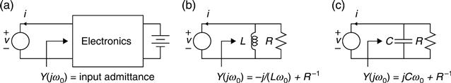
which, through choice of R and L, can be made any magnitude, and any phase in the range [− π/2,0]. Similarly, a feedback law equivalent to a capacitor C in parallel to a resistor R would be
[18.27]
which, through choice of R and C, can be made any magnitude, and any phase in the range [0,π/2]. Because Gi(s) is positive real, it is known that its phase at all frequencies is in the range [− π/2,π/2] and therefore, one of the above two cases always results in a matching circuit for any ω0.
Suppose that the electronics are designed such that their dynamics relate i to v through some causal and stable transfer function, as in Equation [18.23], but not necessarily for the optimal Y(s). Then the closed-loop system is described in the frequency domain, by
[18.28]
[18.29]
where
[18.30]
For the case in which a(t) is characterized by Equation [18.25], the voltage and current in the time domain are
[18.31]
[18.32]
The instantaneous absorbed power is Pabs (t) = − v(t)i(t). Substituting the above, and using some trigonometric identities, we have that
[18.33]
where P and Q are the so-called real and reactive energy flows, defined as
[18.34]
[18.35]
Note that on average, the reactive power oscillates about zero, while the real power has a mean value of P. This is the average power generation in monochromatic response.
Evaluating the value of P at the optimized Y(jω) = Gi− 1(− jω) gives the physical limit on generated power, as
[18.36]
This is the fundamental limit on power generation for monochromatic disturbances. Meanwhile, the reactive power with the optimal feedback is
[18.37]
From Equation [18.33], we see that if | Q | is large, this implies that for each oscillatory cycle a significant amount of energy oscillates back and forth between the harvester and the electronics. If Q is zero, on the other hand, energy always flows from the harvester to the electronics. This is advantageous for a few reasons. Firstly, if it is only necessary for the electronics to facilitate energy flow in one direction, the processing circuitry can be simplified. Secondly, even if processing circuitry with bidirectional energy flow is used, the above analysis does not account for the conductive loss in the circuit, and this loss is minimized for a given P, by designing the system such that Q is zero. For this reason, it is often desirable to design the harvester to achieve Q = 0 in the development above by tuning the hardware parameters such that
[18.38]
In other words, the harvester is tuned such that v(t) and i(t) are in phase at the excitation frequency.18,19
One way to accomplish this is through mechanical tuning design. For example, consider the SDOF electromagnetic harvester in Fig. 18.1a. In this case, we have that
[18.39]
[18.40]
Interestingly, Popt does not depend on k at all, and thus the stiffness can be chosen so as to make Qopt = 0. This is done by tuning the harvester so that ![]() . So doing, the optimal Y(jω0) is
. So doing, the optimal Y(jω0) is
[18.41]
Thinking back to the ‘equivalent circuit’ interpretation of the harvesting feedback law, we see that the tuned harvester is equivalent to a resistor (i.e., with no capacitor or inductor in parallel).
To increase Popt for the SDOF electromagnetic harvester, either c must be decreased, or m must be increased. Indeed, Popt can theoretically be made arbitrarily large by designing the harvester to have arbitrarily small damping. This is the reason why most energy harvesters are deliberately designed to have very low damping. However, in actuality there are often other constraints that limit power generation, requiring Y(s) to be different from its theoretically optimal value. For example, for the SDOF electromagnetic harvester, a displacement constraint |x(t)| ≤ x0 may impose a tighter limit on power generation. Using Lagrange multipliers, it can be shown that with this constraint imposed the optimal feedback law is modified to
[18.42]
where
[18.43]
is an added term that enforces the closed-loop amplitude constraint |x(t)| ≤ x0 The resultant constrained optimal power generation is
[18.44]
This expression tells us a lot about the harvesting potential of SDOF systems. Note that for small a0 and nonzero c, the stroke limit is not saturated, and the available power is the ideal limit. For c → 0, the stroke limit is always saturated, and the available power is ![]() . This is also an upper limit on the power generation, when c is finite.
. This is also an upper limit on the power generation, when c is finite.
Sometimes it is difficult or impossible to redesign the mechanical parameters of a VEH system to bring about Im{Gi(jω0)} = 0. In many circumstances, an appealing alternative is to bring this condition about via insertion of the equivalent capacitor or inductor in Fig. 18.2 across the terminals of the transducer. So doing, the new Gi(jω0) with this inserted component absorbed into the harvester model has zero phase at the excitation frequency, and consequently the optimized Y(jω0) is equivalent to a resistor. Indeed, this approach is often much easier than mechanical tuning techniques. Its primary disadvantage is that sometimes the particular value of L or C necessary to bring about the matching condition is simply unrealistic. This is true, for example, in piezoelectric applications, in which the value of L can be in the thousands of henries. One clever workaround to address this issue is the SSHI circuit, discussed in Section 18.4.4.
18.3.3 Fundamental power generation limits for stochastic disturbances
When a(t) is stochastic, analogous causal limits can be found for the average power generation in stationary response. However, the mathematics associated with these limits is more complicated, and involves optimal control theory.20 Nonetheless, there is one very simple but conservative limit that can be stated here, which is useful in sizing harvesters. Suppose that a(t) is extremely broadband, and can justifiably be modeled as white noise with spectral intensity Φa. Then it is a fact that the optimal average power generation is bounded from above by
[18.45]
where m is the total mass of the harvester. It turns out that this limit holds irrespective of the harvester type; i.e., it can be a piezoelectric beam, an SDOF electromagnetic system, or even a harvester with significant nonlinearities such as an electrostatic transduction system. Furthermore, it is true whether the feedback law is linear or nonlinear, and is insurpassable irrespective of the circuitry used.
This simple limit illustrates a rather uncompromising truth about harvesting energy from broadband stochastic disturbances. The only way to raise the limit is to add mass. However, it is also worth noting that most harvesters, when excited by broadband disturbances, would fall well short of this upper limit, due to internal dissipation in the harvester as well as dissipation in the circuitry. Design of stochastic VEH technologies that come anywhere near reaching the above limit is generally quite challenging.
18.4 Power extraction circuits
The theory derived in the previous section constitutes the idealized situation, in which the electronics that interface the transducer with the energy storage can be designed to absorb energy like a linear admittance Y(s). We showed that for a monochromatic disturbance at frequency ω0, it is only necessary for the electronics to have this input admittance at s = jω0. This makes it easy to design the optimal linear admittance as a combination of a resistor with a reactive component (either an inductor or capacitor, depending on the transducer technology and shaking frequency), as illustrated in Fig. 18.2. However, we have not talked about what the energy harvesting electronics actually constitute, or discussed the way in which practical issues complicate matters.
In order to discuss these issues more concisely from an electrical point of view, equivalent circuit representations of harvesters are helpful. Figure 18.3 shows the Thévenin equivalent circuit for an arbitrary harvester, in which e(t) is called the open-circuit voltage. For monochromatic disturbances, it is equal to
[18.46]
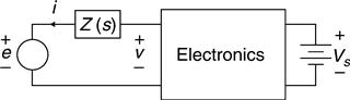
and the electrical impedance Z(s) = Gi(s), as defined in the previous section. If a reactive component has been added to the terminals of the harvester to tune its response, as discussed in the previous section, we assume that this component has been absorbed into the models for Ga and Gi. We refer to a VEH system which has been designed to bring about Im{Gi(jω0)} = 0as a tuned system.
18.4.1 Resistive loads
By far, the most convenient situation in energy harvesting would be where the power generated by the harvester is consumed by a resistive load, with a resistance that can be chosen freely. In this case, the designer would first electrically tune the harvester, if it is not already tuned mechanically, and then simply choose the load resistance to be the optimal R derived from the previous section.
However, the reality of an energy harvesting application is usually much more complicated than this scenario. To start with, it is hardly ever the case that the subsystems for which power is being generated consume this power like a simple resistance, and even less common that the resistance may be treated as a design parameter. For sensing applications, harvested energy is usually delivered to a storage subsystem, consisting of a supercapacitor, rechargeable battery, or some combination of both. Typically, sensing systems operating on harvested energy will spend the majority of the time in a sleep mode, where they consume very little power, during which time the storage bus is trickle charged. Then, periodically, the sensor will come online, conduct measurement, computation, and broadcasting tasks, before returning to sleep mode. As such, the sensing system consumes energy in short bursts of activity, during which time the electronics must maintain a constant voltage on the power bus.
In this context, our energy harvesting analysis from the previous section really pertains to the behavior of the system during the ‘sleep mode’ periods, when the primary objective is to replenish energy storage. During this time, the electronics must facilitate energy transferral from an oscillatory voltage (i.e., e) to the storage device, which typically will possess a positive voltage VS that rises as a slowly varying parameter as the stored energy increases.
18.4.2 The diode bridge rectifier
The simplest (and by far the most prevalent) recharge circuit is a simple full-bridge diode rectifier. This circuit is shown in Fig. 18.4a. Full-bridge rectifiers conduct current when the transducer voltage magnitude |v(t)| exceeds the bus voltage VS plus the diode conduction voltage Vd, and disconnects the transducer from storage otherwise. Assuming VS is a slowly varying parameter, the rectifier imposes a nonlinear relationship between voltage and current, governed by
[18.47]

As such, the rectifier imposes an amplitude saturation on v(t), and draws the current i(t) necessary to ensure this condition. This is illustrated in Fig. 18.4b.
In using a diode bridge rectifier, one would ideally use a capacitor or inductor to tune the harvester. Then, using the method of harmonic balance, an approximately equivalent input resistance Req (i.e., a resistance which absorbs the same energy per cycle) can be found for the electronics, which is shown in Fig. 18.4c. The specific expression for Req is complicated, but the general behavior is that Req for a tuned harvester depends on the ratios (Vs + Vd)/e0 and R0 = Z(jω0 ). As shown in Fig. 18.4d, a fraction of this equivalent resistance (Rd) accounts for the power dissipated by the current as it is transmitted through the rectifier. The remainder of the resistance (R) represents the power absorbed by the storage system. For a tuned harvester, power transferral is optimized with the matching condition
[18.48]
The problem with the diode bridge rectifier is that Req varies over time, as Vs rises, and cannot be controlled. For example, consider the scenario in which the recharge process is initiated at Vs ≈ 0, and assume a0 is sufficiently large such that e0 > Vs + Vd (otherwise, the rectifier will not conduct at all). Then over time, as Vs rises due to the recharge operation, Req will increase from a low initial value at Vs ≈ 0, to infinity when Vs = e0 – Vd. This has two specific drawbacks:
• The rate at which energy is delivered to storage is much lower than the optimal power Popt derived in the last section, because Req will be far from the optimal value for most of the recharge duration. This implies longer recharge times for a desired amount of energy, and inefficient use of the harvester.
• The value of Vs will never exceed e0, no matter how much time the system is given to recharge. Thus, the recharged bus voltage and recovered energy are limited by the level of shaking. For example, if the energy storage device is a supercapacitor with capacitance Cs, the stored energy is limited to ![]() .
.
These drawbacks can limit the usage of the diode bridge rectifier as a recharge circuit. However, for a given application, it makes sense to first assess the typical magnitudes of e0, and the desired recharge rate, and to see if the diode bridge rectifier will be sufficient. It may also be worth considering a redesign of the harvester, expressly to better cope with these limitations. This is because, even though its performance is limited, the full-bridge rectifier does have the distinct advantage of simplicity. In particular, it has no transistors, and does not require control. As such, it is definitely the preferred option for applications where its limitations can be tolerated.
18.4.3 Pulse-width-modulation (PWM)-controlled DC/DC converters
Various techniques have been proposed to overcome the aforementioned drawbacks of the full-bridge rectifier. The central issue is the desire for a recharge circuit with an input impedance that looks like the optimal equivalent resistance R derived in the previous section. Then, by placing a passive reactive component (i.e., an inductor or capacitor) in parallel with this recharge circuit, the input admittance of electronics will look equivalent to one of the circuits in Fig. 18.2, resulting in optimal absorption.
One way to accomplish this is to insert a switch-mode DC/DC converter between the bridge rectifier and the storage bus.21,22 One example of such an implementation, shown in Fig. 18.5a, consists of a MOSFET and diode, together with an inductor, and two capacitors for current filtering. It is controlled by switching the MOSFET on and off, in a PWM cycle. When the MOSFET is switched on, it conducts current, while the diode does not. Alternatively, when the MOSFET is switched off, it appears as an open circuit, and the inductor current flows through the diode. The idea is that by switching the MOSFET on and off periodically at frequency fs = 1/ts, and with duty ratio d, the converter pumps energy from the transducer to the storage bus, using the inductor as an intermediary. Standard procedure is to operate the circuit at a switching frequency which is much higher than the frequency of excitation.

The particular converter shown is called a ‘buck-boost’ converter, because it can transfer power from VR to VS, irrespective of which voltage is the larger. This converter is particularly useful for energy harvesting because, when it is operated in the discontinuous conduction regime (i.e., when the inductor current drops to zero before the end of each PWM cycle), its input impedance is approximately linear and resistive at frequencies well below fs23. More specifically, it turns out that at the excitation frequency, (ω0 the input impedance from the point of view of transducer can be expressed approximately as
[18.49]
where r is a constant that depends primarily on fs and L, but is highly insensitive to VS. As such, the input resistance of the converter can be specified indirectly through proper choice of d, and stays approximately constant as the storage system recharges.24
The use of a DC/DC converter allows for power to be absorbed from the harvester in a manner consistent with the theory in the previous section, i.e., like a resistance. Consequently, the use of such converters in parallel with a tuned inductor or capacitor effectively realizes the linear input admittances in Fig. 18.2. The conductive losses in the MOSFET and diodes can also be taken into account in a manner similar to the way they were for the diode bridge rectifier in the previous subsection, to optimize Req.
However, there are also disadvantages to using DC/DC converters. Most significantly, every time the MOSFET is switched on, its gate capacitance must be charged, and this requires a small amount of energy. Generally, it is not easy to recover this energy when the MOSFET is switched off again. Thus, the gate drive circuit must draw power off of the power bus to run the switching circuit, at a rate that increases with fs. Consequently, fs cannot be too high or else the gating losses become prohibitively high. On the other hand, fs must be kept well above the bandwidth of the harvester in order for the system to operate as intended. As Popt is made smaller, this tradeoff becomes tighter and tighter, and there is ultimately a critical power level below which a given converter is no longer viable. However, the power level where this occurs depends heavily on the specifics of the hardware used, and significant progress is still being made to scale down DC/DC converters to ever-lower power levels for VEH systems.25,26
18.4.4 Synchronized switching circuits
Piezoelectric harvesters possess a significant internal capacitance, and consequently a supplemental inductor L must be attached to the harvester terminals to electrically tune it such that Im{Gi(jω0)} = 0. Often, the magnitude of L can be prohibitively large, with values in the hundreds or even thousands of henries. This makes passive electrical tuning of the harvester impossible. There are several approaches that could be used to address this issue. One is to use a power-electronic converter with bidirectional energy flow capability, in which case both the real and reactive energy flows are facilitated by the converter.27 This approach is theoretically advantageous, but the converter circuitry (and its control) are more complicated and exhibit higher parasitic losses. Another approach is to realize the inductor artificially, using a gyrator circuit. Such circuits use operational amplifiers and capacitors to create the illusion of an inductor. However, it is difficult to make such circuits acceptably efficient at small power scales. A third option, which has received significant attention for energy harvesting applications, involves the use of a synchronized switching circuit.
Figure 18.6 illustrates the insertion of a synchronized switch between a piezoelectric transducer and the DC/DC converter circuit discussed in the previous subsection. This particular circuit is called a parallel synchronized switch harvesting inductor (SSHI) circuit, which was originally proposed for these types of applications in Reference 28. Typically, the inductor used in this circuit is very small, many orders of magnitude lower than that necessary to electrically tune the harvester. The switch in the circuit is realized with a MOSFET and diode. Unlike the PWM-controlled switch used in the DC/DC converter, the switch in the SSHI switch is only triggered twice in a vibratory period of the harvester. Each time, it induces a near-instantaneous polarity reversal in v, thus causing it to have zero crossings at desired times. Through proper switch timing, the phase of the fundamental harmonic of v(t) can be forced to be the same as it would with passive tuning techniques.

Synchronized switching circuits have been shown to be highly effective at greatly enhancing the power generation from monochromatically-excited piezoelectric harvesters.29–33 Especially near resonance, the optimal switch trigger times are nearly coincident with the displacement peaks of the harvester, and consequently, the switching actions can be instigated using a displacement sensor and a simple peak-detection circuit. In contrast to the PWM-controlled switches, the gating losses associated with the SSHI circuits are negligible, because they are only triggered twice in a vibratory cycle. Meanwhile, they have two drawbacks that can in some circumstances reduce their efficiency. First, they conduct current in a short-period pulse each time the switch is triggered, and this can lead to significant conductive dissipation. Second, they introduce significant harmonics into the periodic response, and much of the energy transferred to these higher frequencies is not recovered. More detailed modeling of the losses in SSHI systems can be used to compensate for these losses.32
18.5 Ongoing advancements and future directions
VEH technology continues to be a thriving area of research. We close this chapter with a short (and, to be sure, incomplete) list of three interesting issues currently under investigation by the research community.
18.5.1 Frequency-robust monochromatic energy harvesting
Consider again the optimal power generation limit for a monochromatically-excited SDOF harvester, from Equation [18.39]. As we have discussed, this limit is raised by making c as small as possible, resulting in the general practice of making harvesters very lightly-damped. However, when passive techniques are used to tune the harvester (either mechanically or electrically) this also makes the harvester’s power generation capability extremely narrowband, which can have undesirable ramifications if the frequency ω0 is uncertain. One remedy for this is to deliberately introduce conservative nonlinearities (such as nonlinear stiffnesses) into the electromechanical dynamics of the harvester. If done properly, this can have the effect of creating high-amplitude open-circuit voltages over a wider range of ω0 values. This has led to a flurry of recent activity on nonlinear energy harvesting, as recently summarized in Reference 34.
Rather than engineer mechanical nonlinearities into a harvester to maintain high power levels as ω0 is varied, it can be alternatively done by adapting Y(jω) such that the condition Y(jω0) = Gi–1 (–jω0) is maintained as ω0 slowly varies. This has been investigated recently in Reference 35. Because the reactive power is actively regulated by the electronics, the rectifier and DC/DC converter shown in Fig. 18.5 cannot be used, and must be replaced with a bidirectional converter. This is challenging because bidirectional converters require more elaborate switching control, and generally exhibit higher parasitic losses.
For piezoelectric applications employing SSHI circuits, adaptive tuning can be achieved merely by adapting the phase angle at which the switch is triggered. This has recently been examined in Reference 36.
18.5.2 Broadband stochastic energy harvesting
In many applications, the disturbance a cannot be presumed to be monochromatic, and is much more appropriately modeled as a stochastic process, possibly with a low quality factor. For such cases, determination of the optimal energy harvesting circuit is more challenging because the system must harvest energy from a continuous band of frequencies simultaneously. It should be noted that this problem is fundamentally different from the aforementioned problem in which the disturbance is assumed to be monochromatic but with uncertain frequency. Indeed, it may be the case that a system optimized for one of the two problems performs poorly when applied to the other. A number of recent studies37,38 have investigated stochastic analogies of the development presented here, in which an equivalent circuit for Y(s) is assumed to be a simple R – C and R – L shunt, and a is assumed to be white noise.
However, it has also been shown in Reference 20 that for white-noise-excited harvesters, the optimal power generation is achievable only with active control, i.e., with a bidirectional converter such as a standard H-bridge drive. Furthermore, the determination of the optimal power extraction can be framed as a feedback optimization problem, with the optimal feedback being determined via the solution to an associated linear-quadratic-Gaussian (LQG) control problem. In Reference 39, this analysis is generalized to the case in which a(t) is colored noise of arbitrary quality factor.
18.5.3 More efficient power electronics
It is almost beyond debate that in the near future, the innovations that will have the largest impact on the state-of-the-art in VEH systems will be those that enhance the efficiency of recharge circuits. This is especially true for power levels below about 100 μW. Efficiency improvements may be made by finding ways to reduce the dissipation of energy as it flows from the transducer terminals to storage, especially in the semiconductor components of the circuit. For example, one simple and well-known technique for reducing conductive losses is to replace the rectifier diodes with MOSFETs which are actively switched to behave like diodes. Although some power is required to actively switch these MOSFETs, they dissipate much less energy than diodes at low current levels, and as such, the net energy consumption is reduced. Another well-known approach to reduce losses is to use DC/DC converters that exhibit soft switching, i.e., MOSFETs that are only switched on or off when their current is zero. This reduces the transition losses associated with switching, actions. There are also opportunities to reduce losses in the gate drive circuits for MOSFETs, through the recapture and reuse of the gating energy. This enables the effective use of DC/DC converters at much lower power levels.
Beyond these ideas, which may be viewed as incremental advancements on existing electronics topologies, it is also likely that in very low-power regimes, custom solid-state converter topologies and transmission techniques will be required. For example, energy harvesting circuits at MEMS scale can be built using CMOS-switched capacitors and without inductors (i.e., charge pumps), which can greatly reduce conduction losses. There has been significant advancement in this area over the last ten years, which is summarized in a recent survey by Chao.14 These results suggest that the next decade will see a dramatic expansion in the spectrum of power scales over which VEH systems are viable.