
When the processor runs your programs, it is unlikely that it will start with the first instruction and proceed sequentially through all the instructions in the program until the last instruction. Instead, your program will most likely use branches and loops to perform the necessary logic to implement the functions it needs.
Similar to high-level languages, assembly language provides instructions to help the programmer code logic into applications. By jumping to different sections of the program, or looping through sections multiple times, you can alter the way the program handles data.
This chapter describes the different assembly language instructions used to do jumps and loops. Because both of these functions manipulate the instruction pointer, the first section provides a brief refresher on how the instruction pointer is used to keep track of the next instruction to process, and what instructions can alter the instruction pointer. The next section discusses unconditional branches and demonstrates how they are used in assembly language programs. After that, conditional branches are presented, showing how they can be used to implement logic functions in the application. The next two sections describe loops, special instructions that enable the program to loop through data for a predetermined number of times. Finally, you will learn some tips for optimizing programs that utilize jumps and loops.
Before diving into the details of changing the course of the program, it is a good idea to first understand how the program is executed on the processor. The instruction pointer is the traffic cop for the processor. It determines which instruction in the program is the next in line to be executed. It proceeds in a sequential manner through the instruction codes programmed in the application.
However, as described in Chapter 2, "The IA-32 Platform," it is not always an easy task to determine when and where the next instruction is. With the invention of the instruction prefetch cache, many instructions are preloaded into the processor cache before they are actually ready to be executed. With the invention of the out-of-order engine, many instructions are even executed ahead of time in the application, and the results are placed in order as required by the application by the retirement unit.
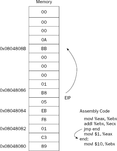
With all of this confusion, it can be difficult to determine what exactly is the "next instruction." While there is a lot of work going on behind the scenes to speed up execution of the program, the processor still needs to sequentially step through the program logic to produce the proper results. Within that framework, the instruction pointer is crucial to determining where things are in the program. This is shown in Figure 6-1.

An instruction is considered executed when the processor retirement unit executes the result from the out-of-order engine from the instruction. After that instruction is executed, the instruction pointer is incremented to the next instruction in the program code. That instruction may or may not have already been performed by the out-of-order engine, but either way, the retirement unit does not process its results until it is time to do so in the program logic.
As the instruction pointer moves through the program instructions, the EIP register is incremented. Remember, instructions can be multiple bytes in length, so pointing to the next instruction is more than just incrementing the instruction pointer by one each time.
Your program cannot directly modify the instruction pointer. You do not have the capability to directly change the value of the EIP register to point to a different location in memory with a MOV instruction. You can, however, utilize instructions that alter the value of the instruction pointer. These instructions are called branches.
A branch instruction can alter the value of the EIP register either unconditionally (unconditional branches), or based on a value of a condition (conditional branches). The following sections describe unconditional and conditional branches and show how they affect the instruction pointer and the course of the program logic.
When an unconditional branch is encountered in the program, the instruction pointer is automatically routed to a different location. You can use three types of unconditional branches:
Each of these unconditional branches behaves differently within the program, and it is up to you to decide which one to use within the program logic. The following sections describe the differences between each of these types of unconditional branches and how to implement them in your assembly language programs.
The jump is the most basic type of branch used in assembly language programming. If you are familiar with the BASIC programming language, you have most likely seen GOTO statements. Jump statements are the assembly language equivalent of the BASIC GOTO statement.
In structured programming, GOTO statements are considered to be a sign of bad coding. Programs are supposed to be compartmentalized and flow in a sequential manner, calling functions instead of jumping around the program code. In assembly language programs, jump instructions are not considered bad programming, and in fact are required to implement many functions. However, they can have a detrimental impact on your program's performance (see "Optimizing Branch Instructions" later in this chapter).
The jump instruction uses a single instruction code:
jmp location
where location is the memory address to jump to. In assembly language, the location value is declared as a label within the program code. When the jump occurs, the instruction pointer is changed to the memory address of the instruction code located immediately after the label. This is shown in Figure 6-2.
The JMP instruction changes the instruction pointer value to the memory location specified in the JMP instruction.
Behind the scenes, the single assembly jump instruction is assembled into one of three different types of jump opcodes:
Short jump
Near jump
Far jump
The three jump types are determined by the distance between the current instruction's memory location and the memory location of the destination point (the "jump to" location). Depending on the number of bytes jumped, the different jump types are used. A short jump is used when the jump offset is less than 128 bytes. A far jump is used in segmented memory models when the jump goes to an instruction in another segment. The near jump is used for all other jumps.
When using the assembly language mnemonic instruction, you do not need to worry about the length of the jump. A single jump instruction is used to jump anywhere in the program code (although there may be a performance difference, as described later in the "Optimizing Branch Instructions" section).
The following jumptest.s program demonstrates the operation of an unconditional jump instruction:
# jumptest.s – An example of the jmp instruction
.section .text
.globl _start
_start:
   nop
   movl $1, %eax
   jmp overhere
   movl $10, %ebx
   int $0x80
overhere:
   movl $20, %ebx
   int $0x80
The jumptest.s program simply assigns the value 1 to the EAX register for the exit Linux system call. Then, a jump instruction is used to jump over the part where the value 10 is assigned to the EBX register, and the Linux system call is made. Instead, the program jumps to where the value 20 is assigned to the EBX register, and the Linux system call is made. You can ensure that the jump occurred by running the program and checking the result code generated in Linux:
$ as -o jumptest.o jumptest.s
$ ld -o jumptest jumptest.o
$ ./jumptest
$ echo $?
20
$
Indeed, the expected result code was produced due to the jump. That in itself might not be too exciting. Instead, you can watch the actual memory locations used in the program with the debugger and the objdump programs.
First, you can see how the instruction codes are arranged in memory by using the objdump program to disassemble the assembled code:
$ objdump -D jumptest

jumptest:     file format elf32-i386

Disassembly of section .text:

08048074 <_start>:
 8048074:       90                      nop
 8048075:       b8 01 00 00 00          mov    $0x1,%eax
 804807a:       eb 07                   jmp    8048083 <overhere>
 804807c:       bb 0a 00 00 00          mov    $0xa,%ebx
 8048081:       cd 80                   int    $0x80

08048083 <overhere>:
 8048083:       bb 14 00 00 00          mov    $0x14,%ebx
 8048088:       cd 80                   int    $0x80
$
The disassembler output shows the memory locations that will be used by each instruction (the value shown in the first column). Now, you can run the jumptest program in the debugger and watch what happens:
$ as -gstabs -o jumptest.o jumptest.s
$ ld -o jumptest jumptest.o
$ gdb -q jumptest
(gdb) break *_start+1
Breakpoint 1 at 0x8048075: file jumptest.s, line 5.
(gdb) run
Starting program: /home/rich/palp/chap06/jumptest

Breakpoint 1, _start () at jumptest.s:5
5          movl $1, %eax
Current language:  auto; currently asm
(gdb) print/x $eip
$1 = 0x8048075
(gdb)
After assembling the code for the debugger (using the -gstabs parameter), and setting the breakpoint at the start of the program, run the program and view the first memory location used (shown in the EIP register). The value is 0x8048075, which corresponds to the same memory location shown in the objdump output. Next, step through the debugger until the jump instruction has been executed, and then display the EIP register value again:
(gdb) step
_start () at jumptest.s:6
6          jmp overhere
(gdb) step
overhere () at jumptest.s:10
10         movl $20, %ebx
(gdb) print $eip
$2 = (void *) 0x8048083
(gdb)
As expected, the program jumped to the 0x8048083 location, which is exactly where the overhere label pointed to, as shown in the objdump output.
The next type of unconditional branch is the call. A call is similar to the jump instruction, but it remembers where it jumped from and has the capability to return there if needed. This is used when implementing functions in assembly language programs.
Functions enable you to write compartmentalized code; that is, you can separate different functions into different sections of the text. If multiple areas of the program use the same functions, the same code does not need to be written multiple times. The single function can be referenced using call statements.
The call instruction has two parts. The first part is the actual CALL instruction, which requires a single operand, the address of the location to jump to:
call address
The address operand refers to a label in the program, which is converted to the memory address of the first instruction in the function.
The second part of the call instruction is the return instruction. This enables the function to return to the original part of the code, immediately after the CALL instruction. The return instruction has no operands, just the mnemonic RET. It knows where to return to by looking at the stack. This is demonstrated in Figure 6-3.
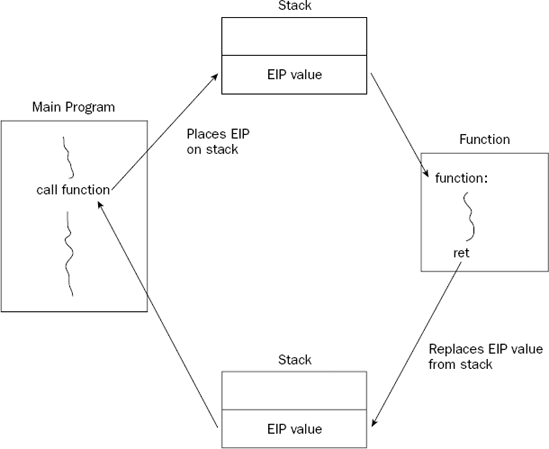
When the CALL instruction is executed, it places the EIP register onto the stack and then modifies the EIP register to point to the called function address. When the called function is completed, it retrieves the old EIP register value from the stack and returns control back to the original program.
How functions return to the main program is possibly the most confusing part of using functions in assembly language. It is not as simple as just using the RET instruction at the end of a function. Instead, it relates to how information is passed to functions and how functions read and store that information.
This is all done using the stack. As mentioned in Chapter 5, "Moving Data," not only can the data on the stack be referenced using PUSH and POP instructions, it can also be directly referenced using the ESP register, which points to the last entry in the stack. Functions normally copy the ESP register to the EBP register, and then use the EBP register value to retrieve information passed on the stack before the CALL instruction, and to place variables on the stack for local data storage (see Chapter 11, "Using Functions"). This complicates how the stack pointer is manipulated within the function.
This is a somewhat simplified explanation of how functions use the stack. Chapter 11, "Using Functions," describes this in great detail, explaining and demonstrating how functions use the stack for data storage.
The return address is added to the stack when the CALL instruction is executed. When the called function begins, it must store the ESP register somewhere it can be restored to its original form before the RET instruction attempts to return to the calling location. Because the stack may also be manipulated within the function, the EBP register is often used as a base pointer to the stack. Thus, the ESP register is usually copied to the EBP register at the beginning of the function as well.
While this seems confusing, it is not too difficult if you create a standard template to use for all of your function calls. The form to remember for functions is as follows:
function_label:
    pushl %ebp
    movl %esp, %ebp
    < normal function code goes here>
    movl %ebp, %esp
    popl %ebp
    ret
Once the EBP register has been saved, it can be used as the base pointer to the stack for all access to the stack within the function. Before returning to the calling program, the ESP register must be restored to the location pointing to the calling memory location.
A simple call example is demonstrated in the calltest.s program:
# calltest.s - An example of using the CALL instruction
.section .data
output:
   .asciz "This is section %d
"
.section .text
.globl _start
_start:
   pushl $1
   pushl $output
   call printf
   add  $8, %esp           # should clear up stack
   call overhere
   pushl $3
   pushl $output
   call printf
   add  $8, %esp           # should clear up stack
   pushl $0
   call exit
overhere:
   pushl %ebp
movl %esp, %ebp
   pushl $2
   pushl $output
   call printf
   add  $8, %esp           # should clear up stack
   movl %ebp, %esp
   popl %ebp
   ret
The calltest.s program begins by using the printf C function to display the first text line, showing where the program is. Next, the CALL instruction is used to transfer control to the overhere label. At the overhere label, the ESP register is copied to the EBP pointer so it can be restored at the end of the function. The printf function is used again to display a second line of text, and then the ESP and EBP registers are restored.
Control of the program returns to the instruction immediately after the CALL instruction, and the third text line is displayed, again using the printf function. The output should look like this:
$ ./calltest
This is section 1
This is section 2
This is section 3
$
Be careful when calling external functions from your application. There is no guarantee that the function will return your registers in the same way that you left them before the call. This is discussed in more detail in Chapter 11.
The third type of unconditional branch is the interrupt. An interrupt is a way for the processor to "interrupt" the current instruction code path and switch to a different path. Interrupts come in two varieties:
Software interrupts
Hardware interrupts
Hardware devices generate hardware interrupts. They are used to signal events happening at the hardware level (such as when an I/O port receives an incoming signal). Programs generate software interrupts. They are a signal to hand off control to another program.
When a program is called by an interrupt, the calling program is put on hold, and the called program takes over. The instruction pointer is transferred to the called program, and execution continues from within the called program. When the called program is complete, it can return control back to the calling program (using an interrupt return instruction).
Software interrupts are provided by the operating system to enable applications to tap into functions within the operating system, and in some cases even the underlying BIOS system. In the Microsoft DOS operating system, many functions are provided with the 0x21 software interrupt. In the Linux world, the 0x80 interrupt is used to provide low-level kernel functions.
You have already seen several examples of using the software interrupt in many of the example programs presented so far. Simply using the INT instruction with the 0x80 value transfers control to the Linux system call program. The Linux system call program has many subfunctions that can be used. The subfunctions are performed based on the value of the EAX register at the time of the interrupt. For example, placing the value of 1 in the EAX register before the interrupt calls the exit Linux system call function.
Chapter 12, "Using Linux System Calls," describes all of the functions available with the 0x80 interrupt.
When debugging an application that contains software interrupts, it is difficult to see what is happening within the interrupt section, as the debugging information is not compiled into the functions. You may have noticed when running the debugger that it performs the interrupt instruction but then immediately returns back to the normal program.
Unlike unconditional branches, conditional branches are not always taken. The result of the conditional branch depends on the state of the EFLAGS register at the time the branch is executed.
There are many bits in the EFLAGS register, but the conditional branches are only concerned with five of them:
Carry flag (CF) - bit 0 (lease significant bit)
Overflow flag (OF) - bit 11
Parity flag (PF) - bit 2
Sign flag (SF) - bit 7
Zero flag (ZF) - bit 6
Each conditional jump instruction examines specific flag bits to determine whether the condition is proper for the jump to occur. With five different flag bits, several jump combinations can be performed. The following sections describe the individual jump instructions.
The conditional jumps determine whether or not to jump based on the current value of the EFLAGS register. Several different conditional jump instructions use different bits of the EFLAGS register. The format of the conditional jump instruction is
jxx address
where xx is a one- to three-character code for the condition, and address is the location within the program to jump to (usually denoted by a label). The following table describes all of the conditional jump instructions available.
Description | EFLAGS | |
|---|---|---|
Jump if above | CF=0 and ZF=0 | |
Jump if above or equal | CF=0 | |
Jump if below | CF=1 | |
Jump if below or equal | CF=1 or ZF=1 | |
Jump if carry | CF=1 | |
Jump if CX register is 0 | ||
Jump if ECX register is 0 | ||
JE | Jump if equal | ZF=1 |
Jump if greater | ZF=0 and SF=OF | |
Jump if greater or equal | SF=OF | |
Jump if less | SF<>OF | |
Jump if less or equal | ZF=1 or SF<>OF | |
Jump if not above | CF=1 or ZF=1 | |
Jump if not above or equal | CF=1 | |
Jump if not below | CF=0 | |
Jump if not below or equal | CF=0 and ZF=0 | |
Jump if not carry | CF=0 | |
Jump if not equal | ZF=0 | |
Jump if not greater | ZF=1 or SF<>OF | |
Jump if not greater or equal | SF<>OF | |
Jump if not less | SF=OF | |
Jump if not less or equal | ZF=0 and SF=OF | |
Jump if not overflow | OF=0 | |
Jump if not parity | PF=0 | |
Jump if not sign | SF=0 | |
Jump if not zero | ZF=0 | |
Jump if overflow | OF=1 | |
Jump if parity | PF=1 | |
Jump if parity even | PF=1 | |
Jump if parity odd | PF=0 | |
Jump if sign | SF=1 | |
Jump if zero | ZF=1 |
You may notice that many of the conditional jump instructions seem redundant (such as JA for jump if above and JG jump if greater). The difference is when working with signed and unsigned values. The jump instructions using the above and lower keywords are used for evaluating unsigned integer values. You will learn more about the different types of integers in Chapter 7, "Using Numbers."
The conditional jump instructions take a single operand in the instruction code—the address to jump to. While usually a label in an assembly language program, the operand is converted into an offset address in the instruction code. Two types of jumps are allowed for conditional jumps:
Short jumps
Near jumps
A short jump uses an 8-bit signed address offset, whereas a near jump uses either a 16-bit or 32-bit signed address offset. The offset value is added to the instruction pointer.
Conditional jump instructions do not support far jumps in the segmented memory model. If you are programming in the segmented memory model, you must use programming logic to determine whether the condition exists, and then implement an unconditional jump to the instructions in the separate segment.
To be able to use a conditional jump, you must have an operation that sets the EFLAGS register before the conditional jump. The next section shows some examples of using conditional jumps in assembly language programs.
The compare instruction is the most common way to evaluate two values for a conditional jump. The compare instruction does just what its name says, it compares two values and sets the EFLAGS registers accordingly.
The format of the CMP instruction is as follows:
cmp operand1, operand2
The CMP instruction compares the second operand with the first operand. It performs a subtraction operation on the two operands behind the scenes (operand2 – operand1). Neither of the operands is modified, but the EFLAGS register is set as if the subtraction took place.
When using the GNU assembler, remember that
operand1andoperand2are the reverse from what is described in the Intel documentation for theCMPinstruction. This little feature has caused many hours of debugging nightmares for many an assembly language programmer.
The following cmptest.s program is shown as a quick demonstration of how the compare and conditional jump instructions work together:
# cmptest.s - An example of using the CMP and JGE instructions
.section .text
.globl _start
_start:
   nop
   movl $15, %eax
   movl $10, %ebx
   cmp %eax, %ebx
   jge greater
   movl $1, %eax
   int $0x80
greater:
   movl $20, %ebx
   movl $1, %eax
   int $0x80
The cmptest.s program first assigns to immediate data values: the value 15 to the EAX register, and the value 10 to the EBX register. Next, the CMP instruction is used to compare the two registers, and the JGE instruction is used to branch, depending on the values:
cmp %eax, %ebx
jge greater
Because the value of the EBX register is less than the value of EAX, the conditional branch is not taken. The instruction pointer moves on to the next instruction, which moves the immediate value of 1 to the EAX register, and then calls the Linux exit system call. You can test this by running the program and displaying the result code:
$ ./cmptest
$ echo $?
10
$
Indeed, the branch was not taken, and the value in the EBX register remained at 10.
The preceding example compared the values of two registers. Following are some other examples of the CMP instruction:
cmp $20, %ebx     ; compare EBX with the immediate value 20
cmp data, %ebx   ; compare EBX with the value in the data memory location
cmp (%edi), %ebx ; compare EBX with the value referenced by the EDI pointer
Trying to code conditional jump instructions can be tricky. It helps to have an understanding of each of the flag bits that must be present in order for the different conditions to be met. The following sections demonstrate how each of the flag bits affect the conditional jumps, so you can get a feeling for what to look for when coding your programming logic.
The Zero flag is the easiest thing to check when doing conditional jumps. The JE and JZ instructions both branch if the Zero flag is set (the two operands are equal). The Zero flag can be set by either a CMP instruction or a mathematical instruction that evaluates to Zero, as shown in the following example:
movl $30, %eax
subl $30, %eax
jz overthere
The JZ instruction would be performed, as the result of the SUB instruction would be Zero (the SUB instruction is covered in Chapter 8, "Basic Math Functions").
You can also use the Zero flag when decreasing the value of a register to determine whether it has reached Zero:
movl $10, %edi
loop1:
   < other code instructions>
   dec %edi
   jz out
   jmp loop1
out:
This code snippet uses the EDI register as an indexed counter that counts back from 10 to 1 (when it reaches zero, the JZ instruction will exit the loop).
The overflow flag is used specifically when working with signed numbers (see Chapter 7). It is set when a signed value is too large for the data element containing it. This usually happens during arithmetic operations that overflow the size of the register holding the data, as shown in the following example:
movl $1, %eax      ; move 1 to the EAX register
   movb $0x7f, %bl    ; move the signed value 127 to the 8-bit BL register
   addb $10, %bl      ; Add 10 to the BL register
   jo overhere
   int $0x80          ; call the Linux system call
overhere:
   movl $0, %ebx      ; move 0 to the EBX register
   int $0x80          ; call the Linux system call
This code snippet adds 10 to a signed byte value of 127. The result would be 137, which is a valid value in the byte, but not within a signed byte number (which can only use −127 to 127). Because the signed value is not valid, the overflow flag is set, and the JO instruction is implemented.
The parity flag indicates the number of bits that should be one in a mathematical answer. This can be used as a crude error-checking system to ensure that the mathematical operation was successful.
If the number of bits set to one in the resultant is even, the parity bit is set (one). If the number of bits set to one in the resultant is odd, the parity bit is not set (zero).
To test this concept, you can create the paritytest.s program:
# paritytest.s - An example of testing the parity flag
.section .text
.globl _start
_start:
   movl $1, %eax
   movl $4, %ebx
   subl $3,  %ebx
   jp overhere
   int $0x80
overhere:
   movl $100, %ebx
   int $0x80
In this snippet, the result from the subtraction is 1, which in binary is 00000001. Because the number of one bits is odd, the parity flag is not set, so the JP instruction should not branch; instead, the program should exit with a result code of the result of the subtraction, 1:
$ ./paritytest
$ echo $?
1
$
To test the opposite, change the SUB instruction line to create a result with an even number of one bits:
subl $1, %ebx
The result of this subtraction will be 3, which in binary is 00000011. Because this is an even number of one bits, the parity flag will be set, and the JP instruction should branch to the overhere label, setting the result code to 100:
$ ./paritytest
$ echo $?
100
$
Yes, it worked as expected!
The sign flag is used in signed numbers to indicate a sign change in the value contained in the register. In a signed number, the last (highest order) bit is used as the sign bit. It indicates whether the numeric representation is negative (set to 1) or positive (set to 0).
This is handy when counting within a loop and watching for zero. You saw with the Zero flag that the flag was set when the value that was being decreased reached zero. However, if you are dealing with arrays, most likely you also need to stop after the zero value, not at the zero value (because the first offset is 0).
Using the sign flag, you can tell when a value has passed from 0 to −1, as shown in the following signtest.s program:
# signtest.s - An example of using the sign flag
.section .data
value:
   .int 21, 15, 34, 11, 6, 50, 32, 80, 10, 2
output:
   .asciz "The value is: %d
"
.section .text
.globl _start
_start:
   movl $9, %edi
loop:
   pushl value(, %edi, 4)
   pushl $output
   call printf
   add $8, $esp
   dec %edi
   jns loop
   movl $1, %eax
   movl $0, %ebx
   int $0x80
The signtest.s program walks backward through a data array using the EDI register as an index, decreasing it for each array element. The JNS instruction is used to detect when the value of the EDI register becomes negative, and loops back to the beginning if not.
Because the signtest.s program uses the printf C function, remember to link it with the dynamic loader (as described in Chapter 4, "A Sample Assembly Language Program"). The output from the program should look like this:
$ ./signtest
The value is: 2
The value is: 10
The value is: 80
The value is: 32
The value is: 50
The value is: 6
The value is: 11
The value is: 34
The value is: 15
The value is: 21
$
The carry flag is used in mathematical expressions to indicate when an overflow has occurred in an unsigned number (remember that signed numbers use the overflow flag). The carry flag is set when an instruction causes a register to go beyond its data size limit.
Unlike the overflow flag, the DEC and INC instructions do not affect the carry flag. For example, this code snippet will not set the carry flag:
movl $0xffffffff, %ebx
inc %ebx
jc overflow
However, this code snippet will set the carry flag, and the JC instruction will jump to the overflow location:
movl $0xffffffff, %ebx
addl $1,  %ebx
jc overflow
The carry flag will also be set when an unsigned value is less than zero. For example, this code snippet will also set the carry flag:
movl $2, %eax
subl $4, %eax
jc overflow
The resulting value in the EAX register is 254, which represents −2 as a signed number, the correct answer. This means that the overflow flag would not be set. However, because the answer is below zero for an unsigned number, the carry flag is set.
Unlike the other flags, there are instructions that can specifically modify the carry flag. These are described in the following table.
Instruction | Description |
|---|---|
CLC | Clear the carry flag (set it to zero) |
CMC | Complement the carry flag (change it to the opposite of what is set) |
Set the carry flag (set it to one) |
Each of these instructions directly modifies the carry flag bit in the EFLAGS register.
Loops are another way of altering the instruction path within the program. Loops enable you to code repetitive tasks with a single loop function. The loop operations are performed repeatedly until a specific condition is met.
The following sections describe the different loop instructions available for you to use and show an example of using loops within an assembly language program.
In the signtest.s example program shown in the section "Using the sign flag," you created a loop by using a jump instruction and decreasing a register value. The IA-32 platform provides a simpler mechanism for performing loops in assembly language programs: the loop instruction family.
The loop instructions use the ECX register as a counter and automatically decrease its value as the loop instruction is executed. The following table describes the instructions in the loop family.
Instruction | |
|---|---|
LOOP | Loop until the ECX register is zero |
LOOPE/LOOPZ | Loop until either the ECX register is zero, or the ZF flag is not set |
LOOPNE/LOOPNZ | Loop until either the ECX register is zero, or the ZF flag is set |
The LOOPE/LOOPZ and LOOPNE/LOOPNZ instructions provide the additional benefit of monitoring the Zero flag.
The format for each of these instructions is
loop address
where address is a label name for a location in the program code to jump to. Unfortunately, the loop instructions support only an 8-bit offset, so only short jumps can be performed.
Before the loop starts, you must set the value for the number of iterations to perform in the ECX register. This usually looks something like the following:
< code before the loop >
   movl $100, %ecx
loop1:
   < code to loop through >
   loop loop1
   < code after the loop >
Be careful with the code inside the loop. If the ECX register is modified, it will affect the operation of the loop. Use extra caution when implementing function calls within the loop, as functions can easily trash the value of the ECX register without you knowing it.
An added benefit of the loop instructions is that they decrease the value of the ECX register without affecting the EFLAGS register flag bits. When the ECX register reaches zero, the Zero flag is not set.
As a simple example to demonstrate how the LOOP instruction works, here's the loop.s program:
# loop.s - An example of the loop instruction
.section .data
output:
   .asciz "The value is: %d
"
.section .text
.globl _start
_start:
   movl $100, %ecx
   movl $0, %eax
loop1:
   addl %ecx, %eax
   loop loop1
   pushl %eax
   pushl $output
   call printf
   add $8, %esp
   movl $1, %eax
   movl $0, %ebx
   int $0x80
The loop.s program computes the arithmetic series of the number stored in the ECX register and then displays it on the console (using the printf function, so remember to link with the C library and the dynamic linker). The LOOP instruction is used to continually loop through the ADD function until the value of ECX is zero.
There is one common problem with the LOOP instruction that sometimes bites assembly language programmers. What if you used the loop.s example program and set the ECX register to zero? Try it and see what happens. Here's the output when I tried it:
$ ./loop
The value is: −2147483648
$
That is obviously not the correct answer. So what happened? The answer lies in the way the LOOP instruction behaves. When the LOOP instruction is executed, it first decreases the value in ECX by one, and then it checks to see whether it is zero. Using this logic, if the value of ECX is already zero before the LOOP instruction, it will be decreased by one, making it −1. Because this value is not zero, the LOOP instruction continues on its way, looping back to the defined label. The loop will eventually exit when the register overflows, and the incorrect value is displayed.
To correct this problem, you need to check for the special condition when the ECX register contains a zero value. Fortunately, Intel has provided a special instruction just for that purpose. If you remember from the "Conditional Branches" section earlier, the JCXZ instruction is used to perform a conditional branch if the ECX register is zero. This is exactly what we need to solve this problem.
The betterloop.s program uses the JCXZ instruction to provide some rudimentary error-checking for the application:
# betterloop.s - An example of the loop and jcxz instructions
.section .data
output:
   .asciz "The value is: %d
"
.section .text
.globl _start
_start:
   movl $0, %ecx
movl $0, %eax
   jcxz done
loop1:
   addl %ecx, %eax
   loop loop1
done:
   pushl %eax
   pushl $output
   call printf
   movl $1, %eax
   movl $0, %ebx
   int $0x80
The betterloop.s program adds a single instruction, the JCXZ instruction, before the loop starts, and a single label to reference the ending instruction codes. Now if the ECX register contains a zero value, the JCXZ instruction catches it, and immediately goes to the output section. Running the program demonstrates that indeed it solves the problem:
$ ./betterloop
The value is: 0
$
If you program in C, C++, Java, or any other high-level language, you probably use a lot of conditional statements that look completely different from the assembly language ones. You can mimic the high-level language functions using the assembly language code you learned in this chapter.
The easiest way to learn how to code high-level functions in assembly language is to see how the assembler does it. The following sections walk through disassembling C language functions to show how they are performed using assembly language.
The most common conditional statement used in high-level languages is the if statement. The following program, ifthen.c, demonstrates how this is commonly used in C programs:
/* ifthen.c – A sample C if-then program */
#include <stdio.h>

int main()
{
   int a = 100;
   int b = 25;
   if (a > b)
   {
      printf("The higher value is %d
", a);
   } else
      printf("The higher value is %d
", b);
return 0;
}
Because the purpose of this exercise is to see how the code will be converted to assembly language, the actual C program is pretty trivial—just a simple comparison of two known values. You can view the generated assembly language code by using the -S parameter of the GNU compiler:
$ gcc -S ifthen.c
$ cat ifthen.s
        .file   "ifthen.c"
        .section        .rodata
.LC0:
        .string "The higher value is %d
"
        .text
.globl main
        .type   main, @function
main:
        pushl   %ebp
        movl    %esp, %ebp
        subl    $24, %esp
        andl    $-16, %esp
        movl    $0, %eax
        subl    %eax, %esp
        movl    $100, −4(%ebp)
        movl    $25, −8(%ebp)
        movl    −4(%ebp), %eax
        cmpl    −8(%ebp), %eax
        jle     .L2
        movl    −4(%ebp), %eax
        movl    %eax, 4(%esp)
        movl    $.LC0, (%esp)
        call    printf
        jmp     .L3
.L2:
movl −8(%ebp), %eax
movl %eax, 4(%esp)
movl $.LC0, (%esp)
call printf
.L3:
movl $0, (%esp)
call exit
.size main, .-main
.section .note.GNU-stack,"",@progbits
.ident "GCC: (GNU) 3.3.2 (Debian)"
$That's a lot of assembly code for a simple C function! Now you can see why I wanted to keep the C code simple. Now we can walk through the code step by step to see what it is doing.
The first section of the code:
pushl   %ebp
movl    %esp, %ebp
subl    $24, %esp
andl    $-16, %esp
movl    $0, %eax
subl    %eax, %esp
stores the EBP register so it can be used as a pointer to the local stack area in the program. The stack pointer, ESP, is then manually manipulated to make room for putting local variables on the stack.
The next section of the code creates the two variables used in the If statement:
movl    $100, −4(%ebp)
movl    $25, −8(%ebp)
The first instruction manually moves the value for the a variable into a location on the stack (4 bytes in front of the location pointed to by the EBP register). The second instruction manually moves the value for the b variable into the next location on the stack (8 bytes in front of the location pointed to by the EBP register). This technique, commonly used in functions, is discussed in Chapter 11. Now that both variables are stored on the stack, it's time to execute the if statement:
movl    −4(%ebp), %eax
cmpl    −8(%ebp), %eax
jle     .L2
First, the value for the a variable is moved to the EAX register, and then that value is compared to the value for the b variable, still in the local stack. Instead of looking for the if condition a > b, the assembly language code is looking for the opposite, a <= b. If the statement evaluates to "true," the jump to the .L2 label is made, which is the "else" part of the If statement:
.L2:
    movl    −8(%ebp), %eax
    movl    %eax, 4(%esp)
    movl    $.LC0, (%esp)
    call    printf
This is the code to print the answer for the b variable, which was contained in the else part of the If statement. First the b variable value is retrieved and manually placed on the stack, and then the location of the output text (located at the .LC0 label) is placed on the stack. With both elements on the stack, the printf C function is called to display the answer. The code then proceeds to the ending instructions.
If the JLE instruction was false, then a is not less than or equal to b, and the jump is not performed. Instead, the "then" part of the If statement is performed:
movl    −4(%ebp), %eax
movl    %eax, 4(%esp)
movl    $.LC0, (%esp)
call    printf
jmp     .L3
Here, the a variable is loaded onto the stack, along with the output text. Then the printf C function is called to display the answer, and execution jumps to the .L3 label. Finally, all roads load to the exit C function:
.L3:
    movl    $0, (%esp)
    call    exit
    .size   main, .-main
    .section        .note.GNU-stack,"",@progbits
    .ident  "GCC: (GNU) 3.3.2 (Debian)"
It is pretty easy to see the if-then logic contained in the assembly language code. You can apply the same logic to any if-then situation you need in your assembly language programs.
At first it may appear that the implementation of the if-then logic in assembly language is backwards. It might seem to be easier for the jump instruction to evaluate for the "true" condition to jump to the "then" section. There is a reason why the opposite situation is used, which is shown in the "Optimizing Branch Instructions" section later in this chapter.
The assembly language code used to implement an if statement looks like the following:
if:
   <condition to evaluate>
   jxx  else        ; jump to the else part if the condition is false
<code to implement the "then" statements>
jmp end             ;jump to the end
else:
   < code to implement the "else" statements>
end:
Of course, this was a trivial example of an If statement. In a real production program, the condition to evaluate becomes much more complicated. In these situations, evaluating the condition for the if statement becomes just as crucial as the If statement code itself.
Instead of a single conditional jump instruction, there may be several, with each one evaluating a separate part of the if condition. For example, the C language if statement
if (eax < ebx) || (eax == ecx) then
creates the following assembly language code:
if:
   cmpl %eax, %ebx
   jle else
   cmpl %eax, %ecx
   jne else
then:
   < then logic code>
   jmp end
else:
   < else logic code >
end:
This If statement condition required two separate CMP instructions. Because the logical operator is an OR, if either CMP instruction evaluates to true, the program jumps to the else label. If the logical operator is an AND, you would need to use an intermediate label to ensure that both CMP instructions evaluate to true.
The next statement to tackle is for loops. Here's the sample C program used to start us off, the for.c program:
/* for.c – A sample C for program */
#include <stdio.h>

int main()
{
   int i = 0;
   int j;
   for (i = 0; i < 1000; i++)
   {
      j = i * 5;
      printf("The answer is %d
", j);
   }
return 0;
}
Again, this uses a pretty simplistic C program to demonstrate how for-next loops are implemented in assembly language code. Here's the assembly code generated by the GNU compiler:
$ gcc -S for.c
$ cat for.s
        .file   "for.c"
        .section        .rodata
.LC0:
        .string "The answer is %d
"
        .text
.globl main
        .type   main, @function
main:
pushl %ebp
movl %esp, %ebp
subl $24, %esp
andl $-16, %esp
movl $0, %eax
subl %eax, %esp
movl $0, −4(%ebp)
movl $0, −4(%ebp)
.L2:
    cmpl    $999, −4(%ebp)
    jle     .L5
    jmp     .L3
.L5:
    movl    −4(%ebp), %edx
    movl    %edx, %eax
sall    $2, %eax
    addl    %edx, %eax
    movl    %eax, −8(%ebp)
    movl    −8(%ebp), %eax
    movl    %eax, 4(%esp)
    movl    $.LC0, (%esp)
    call    printf
leal    −4(%ebp), %eax
incl    (%eax)
jmp     .L2
.L3:
movl $0, (%esp)
call exit
.size main, .-main
.section .note.GNU-stack,"",@progbits
.ident "GCC: (GNU) 3.3.2 (Debian)"
$Similar to the if statement code, the for statement code first does some housekeeping with the ESP and EBP registers, manually setting the EBP register to the start of the stack, and making room for the variables used in the function. The for statement starts with the .L2 label:
.L2:
cmpl $999, −4(%ebp)
jle .L5
jmp .L3The condition set in the for statement is set at the beginning of the loop. In this case, the condition is to determine whether the variable is less than 1,000. If the condition is true, execution jumps to the .L5 label, where the for loop code is. When the condition is false, execution jumps to the .L3 label, which is the ending code.
The For loop code is as follows:
.L5:
movl −4(%ebp), %edx
movl %edx, %eaxsall $2, %eax
addl %edx, %eax
movl %eax, −8(%ebp)
movl −8(%ebp), %eax
movl %eax, 4(%esp)
movl $.LC0, (%esp)
call printfThe first variable location (the i variable in the C code) is moved to the EDX register, and then moved to the EAX register. The next two instructions are mathematical operations (which are covered in detail in Chapter 8). The CALL instruction performs a left shift of the EAX register two times. This is equivalent to multiplying the number in the EAX register by 4. The next instruction adds the EDX register value to the EAX register value. Now the EAX register contains the original value multiplied by 5 (tricky).
After the value has been multiplied by 5, it is stored in the location reserved for the second variable (the j variable in the C code). Finally, the value is placed on the stack, along with the location of the output text, and the printf C function is called.
The next part of the code gets back to the for statement function:
leal −4(%ebp), %eax incl (%eax) jmp .L2
The LEA instruction has not been discussed yet. It loads the effective memory address of the declared variable into the register specified. Thus, the memory location of the first variable (i) is loaded into the EAX register. The next instruction uses the indirect addressing mode to increment the value pointed to by the EAX register by one. This in effect adds one to the i variable. After that, execution jumps back to the start of the for loop, where the I value will be tested to determine whether it is less than 1,000, and the whole process is performed again.
From this example you can see the framework for implementing for loops in assembly language. The pseudocode looks something like this:
for:
   <condition to evaluate for loop counter value>
   jxx forcode    ; jump to the code of the condition is true
   jmp end        ; jump to the end if the condition is false
forcode:
  < for loop code to execute>
  <increment for loop counter>
   jmp for        ; go back to the start of the For statement
end:
The
whileloop code uses a format similar to the For loop code. Try creating a testwhileloop in a C program and viewing the generated assembly code. It will look similar to theforloop code shown here.
Branch instructions greatly impact the performance of applications. Most modern processors (including ones in the IA-32 family) utilize instruction prefetch caches to increase performance. As the program is run, the instruction prefetch cache is filled with sequential instructions.
As described in Chapter 2, the out-of-order engine attempts to execute instructions as soon as possible, even if earlier instructions in the program have not yet been executed. Branch instructions, however, create great havoc in the out-of-order engine. The following sections describe how modern Pentium processors handle branches, and what you can do to improve the performance of your assembly language programs.
When a branch instruction is encountered, the processor out-of-order engine must determine the next instruction to be processed. The out-of-order unit utilizes a separate unit called the branch prediction front end to determine whether or not a branch should be followed. The branch prediction front end employs different techniques in its attempt to predict branch activity. When creating assembly language code that includes conditional branches, you should be aware of this processor feature.
With unconditional branches, the next instruction is not difficult to determine, but depending on how long of a jump there was, the next instruction may not be available in the instruction prefetch cache. This is demonstrated in Figure 6-4.
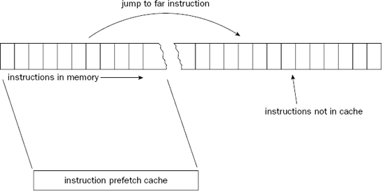
When the new instruction location is determined in memory, the out-of-order engine must first determine if the instruction is available in the prefetch cache. If not, the entire prefetch cache must be cleared, and reloaded with instructions from the new location. This can be costly to the performance of the application.
Conditional branches present an even greater challenge to the processor. For each unconditional branch, the branch prediction unit must determine if the branch should be taken or not. Usually, when the out-of-order engine is ready to execute the conditional branch, not enough information is available to know for certain which direction the branch will take.
Instead, the branch prediction algorithms attempt to guess which path a particular conditional branch will take. This is done using rules and learned history. Three main rules are implemented by the branch prediction algorithms:
Backward branches are assumed to be taken.
Forward branches are assumed to be not taken.
Branches that have been previously taken are taken again.
Using normal programming logic, the most often seen use of backward branches (branches that jump to previous instruction codes) is in loops. For example, the code snippet
movl $100, $ecx
loop1:
   addl %cx, %eax
   decl %ecx
   jns loop1
will jump 100 times back to the loop1 label, but fall through to the next instruction only once. The first branching rule will always assume that the backwards branch will be taken. Out of the 101 times the branch is executed, it will only be wrong once.
Forward branches are a little trickier. The branch prediction algorithm assumes that most of the time conditional branches that go forward are not taken. In programming logic, this assumes that the code immediately following the jump instruction is most likely to be taken, rather than the jump that moves over the code. This situation is seen in the following code snippet:
movl    −4(%ebp), %eax
    cmpl    −8(%ebp), %eax
    jle     .L2
    movl    −4(%ebp), %eax
    movl    %eax, 4(%esp)
    movl    $.LC0, (%esp)
    call    printf
    jmp     .L3
.L2:
    movl    −8(%ebp), %eax
    movl    %eax, 4(%esp)
    movl    $.LC0, (%esp)
call printf .L3:
Does this look familiar? It is the code snippet from the analysis of the C program If statement. The code following the JLE instruction handles the "then" part of the If statement. From a branch prediction point of view, we can now see the reason why the JLE instruction was used instead of a JG instruction. When the compiler created the assembly language code, it attempted to maximize the code's performance by guessing that the "then" part of the If statement would be more likely to be taken than the "else" part. Because the processor branch prediction unit assumes forward jumps to not be taken, the "then" code would already be in the instruction prefetch cache, ready to be executed.
The final rule implies that branches that are performed multiple times are likely to follow the same path the majority of the time. The Branch Target Buffer (BTB) keeps track of each branch instruction performed by the processor, and the outcome of the branch is stored in the buffer area.
The BTB information overrides either of the two previous rules for branches. For example, if a backward branch is not taken the first time it is encountered, the branch prediction unit will assume it will not be taken any subsequent times, rather than assume that the backwards branch rule would apply.
The problem with the BTB is that it can become full. As the BTB becomes full, looking up branch results takes longer, and performance for executing the branch decreases.
While the processor tries its best to optimize how it handles branches, you can incorporate a few tricks into your assembly language programs to help it along. The following sections describe some of the branch optimization tricks recommended by Intel for use on the Pentium family of processors.
The most obvious way to solve branch performance problems is to eliminate the use of branches whenever possible. Intel has helped in this by providing some specific instructions.
In Chapter 5, "Moving Data," the CMOV instructions were discussed. These instructions were specifically designed to help the assembly language programmer avoid using branches to set data values. An example of using a CMOV instruction is as follows:
movl value, %ecx
cmpl %ebx, %ecx
cmova %ecx, %ebx
The CMOVA instruction checks the results from the CMP instruction. If the unsigned integer value in the ECX register is above the unsigned integer value in the EBX register, the value in the ECX register is placed in the EBX register. This functionality enabled us to create the cmovtest.s program, which determined the largest number in a series without a bunch of jump instructions.
Sometimes duplicating a few extra instructions can eliminate a jump. This small instruction overhead will easily fit into the instruction prefetch cache, and make up for the performance hit of the jump itself. A classic example of this is the situation in which a branch can occur within a loop:
loop:
   cmp data(, %edi, 4), %eax
   je part2
   call function1
   jmp looptest
part2:
   call function2
looptest:
   inc %edi
   cmpl $10, %edi
   jnz loop
The loop calls one of two functions, depending on the value read from the data array. After the function is called, a jump is made to the end of the loop to increase the index value of the array and loop back to the start of the loop. Each time the first function is called, the JMP instruction must be evaluated to jump forward to the looptest label. Because this is a forward branch, it will not be predicted to be taken, and a performance penalty will result.
To change this, you can modify the code snippet to look like the following:
loop:
   cmp data(, %edi, 4), %eax
   je part2
   call function1
   inc %edi
   cmp $10, %edi
   jnz loop
   jmp end
part2:
   call function2
   inc %edi
   cmp $10, %edi
   jnz loop
end:
Instead of using the forward branch within the loop, the looptest code was duplicated within the first function code section, eliminating one forward jump from the code.
You can exploit the branch prediction unit rules to increase the performance of your application. As seen in the If statement code presented, placing code that is most likely to be taken as the fall-through of the jump forward statement increases the likelihood that it will be in the instruction prefetch cache when needed. Allow the jump instruction to jump to the less likely used code segments.
For code using backward branches, try to use the backward branch path as the most taken path. When implementing loops this is not usually a problem. However, in some cases you may have to alter the program logic to accomplish this.
Figure 6-5 sums up both of these scenarios.

While loops are generally covered by the backward branch rule, there is still a performance penalty even when they are predicted correctly. A better rule-of-thumb to use is to eliminate small loops whenever possible.
The problem appears in loop overhead. Even a simple loop requires a counter that must be checked for each iteration, and a jump instruction that must be evaluated. Depending on the number of program logic instructions within the loop, this can be a huge overhead.
For smaller loops, unrolling the loop can solve this problem. Unrolling the loop means to manually code each of the instructions multiple times instead of using the loop to go back over the same instruction. The following code is an example of a small loop that can be unrolled:
movl values, %ebx
   movl $1, %edi
loop:
   movl values(, %edi, 4), %eax
   cmp %ebx, %eax
   cmova %eax, %ebx
   inc %edi
   cmp $4, %edi
   jne loop
This was the main loop from the cmovtest.s program in Chapter 5. Instead of looping through the instructions to look for the largest value four times, you can unroll the loop into a series of four moves:
movl values, %ebx
movl $values, %ecx
movl (%ecx), %eax
cmp %ebx, %eax
cmova %eax, %ebx
movl 4(%ecx), %eax
cmp %ebx, %eax
cmova %eax, %ebx
movl 8(%ecx), %eax
cmp %ebx, %eax
cmova %eax, %ebx
movl 12(%ecx), %eax
cmp %ebx, %eax
cmova %eax, %ebx
While the number of instructions has greatly increased, the processor will be able to feed all of them directly into the instruction prefetch cache, and zip through them in no time.
Be careful when unrolling loops though, as it is possible to unroll too many instructions, and fill the prefetch cache. This will force the processor to constantly fill and empty the prefetch cache.
This chapter presented instructions to help you program logic into your assembly language programs. Just about every assembly language program needs the capability to branch to other parts of the instruction code depending on data values, or to loop through sections of code a specific number of times.
The IA-32 platform provides several instructions for coding branching and looping functions. There are two different types of branch functions: unconditional branches and conditional branches. Unconditional branches are performed regardless of external values or events, whereas conditional branches rely on an external value or event to branch.
There are three types of unconditional branches: jumps, calls, and interrupts. The unconditional jump is the most basic form of execution control. The JMP instruction forces the instruction pointer to change to the destination location, and the processor executes the next instruction at that spot. Calls are similar to jumps, but support the capability to return to the location after the call. The return location is stored in the stack area, and the called function must restore the stack back to its original condition before returning to the calling area. Software interrupts are used to provide access to low-level kernel functions in the operating system. Both Microsoft Windows and Linux provide system calls via software interrupts. The Linux system calls are available at software interrupt 0x80.
Conditional branches rely on the values of the EFLAGS register. Specifically, the carry, overflow, parity, sign, and Zero flags are used to affect the conditional branch. Specific branch instructions monitor specific flag bits, such as the JC instruction jumps when the carry flag is set, and the JZ instruction jumps when the Zero flag is set. The CMP instruction is helpful in comparing two values and setting EFLAGS bits for the conditional jump instruction.
Loops provide a method for you to easily replicate code functions without having to duplicate a lot of code. Just as in high-level languages, loops enable you to perform tasks a specific number of times by using a counter value that is decreased for each iteration. The LOOP instruction automatically uses the ECX register as the counter, and decreases and tests it during each iteration.
You can duplicate high-level language conditional functions such as If-then and For statements using common assembly language jumps and loops. To see how C functions are coded, you can use the -S parameter of the GNU compiler to view the generated assembly language code.
When working with Pentium processors, you can use some optimization techniques to increase the performance of your assembly language code. Pentium processors use the instruction prefetch cache, and attempt to load instructions as quickly as possible into the cache. Unfortunately, branch instructions can have a detrimental effect on the prefetch cache. As branches are detected in the cache, the out-of-order engine attempts to predict what path the branch is most likely to take. If it is wrong, the instruction prefetch cache is loaded with instructions that are not used, and processor time is wasted. To help solve this problem, you should be aware of how the processor predicts branches, and attempt to code your branches in the same manner. Also, eliminating branches whenever possible will greatly speed things up. Finally, examining loops and converting them into a sequential series of operations enables the processor to load all of the instructions into the prefetch cache, and not have to worry about branching for the loop.
The next chapter discusses how the processor deals with various types of numbers. Just as in high-level languages, there are multiple ways to represent numbers, and there are multiple ways that those numbers are handled in assembly language programs. Knowing all the different types of number formats can help you when working with mathematically intensive operations.