To create assembly language programs, obviously you need some tool to convert the assembly language source code to instruction code for the processor. This is where the assembler comes in.

As mentioned in Chapter 1, "What Is Assembly Language?," assemblers are specific to the underlying hardware platform for which you are programming. Each processor family has its own instruction code set. The assembler you select must be capable of producing instruction codes for the processor family on your system (or the system you are developing for).

The assembler produces the instruction codes from source code created by the programmer. If you remember from Chapter 1, there are three components to an assembly language source code program:

Unfortunately, each assembler uses different formats for each of these components. Programming using one assembler may be totally different from programming using another assembler. While the basics are the same, the way they are implemented can be vastly different.

The biggest difference between assemblers is the assembler directives. While opcode mnemonics are closely related to processor instruction codes, the assembler directives are unique to the individual assembler. The directives instruct the assembler how to construct the instruction code program. While some assemblers have a limited number of directives, some have an extensive number of directives. Directives do everything from defining program sections to implementing if-then statements or while loops.

You may also have to take into consideration how you will write your assembly language programs. Some assemblers come complete with built-in editors that help recognize improper syntax while you are typing the code, while others are simply command-line programs that can only assemble an existing code text file. If the assembler you choose does not contain an editor, you must select a good editor for your environment. While using the UNIX vi editor can work for simple programs, you probably wouldn't want to code a 10,000-line assembly program using it.

The bottom line for choosing an assembler is its ability to make creating an instruction code program for your target environment as simple as possible. The next sections describe some common assemblers that are available for the Intel IA-32 platform.

If you are familiar with a high-level language environment, it is possible that you have never had to directly use a linker. Many high-level languages such as C and C++ perform both the compile and link steps with a single command.

The process of linking objects involves resolving all defined functions and memory address labels declared in the program code. To do this, any external functions, such as the C language printf function, must be included with the object code (or a reference made to an external dynamic library). For this to work automatically, the linker must know where the common object code libraries are located on the computer, or the locations must be manually specified with compiler command-line parameters.

However, most assemblers do not automatically link the object code to produce the executable program file. Instead, a second manual step is required to link the assembly language object code with other libraries and produce an executable program file that can be run on the host operating system. This is the job of the linker.

When the linker is invoked manually, the developer must know which libraries are required to completely resolve any functions used by the application. The linker must be told where to find function libraries and which object code files to link together to produce the resulting file.

If you are a perfect programmer, you will never need to use a debugger. However, it is more likely that somewhere in your assembly language programming future you will make a mistake — either a small typo in your 10,000-line program, or a logic mistake in your mathematical algorithm functions. When this happens, it is handy to have a good debugger available in your toolkit.

Similar to assemblers, debuggers are specific to the operating system and hardware platform for which the program was written. The debugger must know the instruction code set of the hardware platform, and understand the registers and memory handling methods of the operating system.

Most debuggers provide four basic functions to the programmer:

The debugger runs the program within its own controlled "sandbox." The sandbox enables the program to access memory areas, registers, and I/O devices, but all under the control of the debugger. The debugger is able to control how the program accesses items and can display information about how and when the program accesses the items.

At any point during the execution of the program, the debugger is able to stop the program and indicate where in the source code the execution was stopped. To accomplish this, the debugger must know the original source code and what instruction codes were generated from which lines of source code. The debugger requires additional information to be compiled into the executable file to identify these elements. Using a specific command-line parameter when the program is compiled or assembled usually accomplishes this task.

When the program is stopped during execution, the debugger is able to display any memory area or register value associated with the program. Again, this is accomplished by running the program within the debugger's sandbox, enabling the debugger to peek inside the program as it is executing. By being able to see how individual source code statements affect the values of memory locations and registers, the programmer can often see where an error in the program occurs. This feature is invaluable to the programmer.

Finally, the debugger provides a means for the programmer to change data values within the program as it is executing. This enables the programmer to make changes to the program as it is running and see how the changes affect the outcome of the program. This is another invaluable feature, saving the time of having to change values in source code, recompiling the source code, and rerunning the executable program file.

If all you plan to do is program in assembly language, a high-level language compiler is not necessary. However, as a professional programmer, you probably realize that creating full-blown applications using only assembly language, although possible, would be a massive undertaking.

Instead, most professional programmers attempt to write as much of the application as possible in a high-level language, such as C or C++, and concentrate on optimizing the trouble spots using assembly language programming. To do this, you must have the proper compiler for your high-level language.

The compiler's job is to convert the high-level language into instruction code for the processor to execute. Most compilers, though, produce an intermediate step. Instead of directly converting the source code to instruction code, the compiler converts the source code to assembly language code. The assembly language code is then converted to instruction code, using an assembler. Many compilers include the assembler process within the compiler, although not all do.

After converting the C or C++ source code to assembly language, the GNU compiler uses the GNU assembler to produce the instruction codes for the linker. You can stop the process between these steps and examine the assembly language code that is generated from the C or C++ source code. If you think something can be optimized, the generated assembly language code can be modified, and the code assembled into new instruction codes.

When trying to optimize a high-level language, it usually helps to see how that code is being run on the processor. To do that you need a tool to view the instruction code that is generated by the compiler from the high-level language source code. The GNU compiler enables you to view the generated assembly language code before it is assembled, but what about after the object file is already created?

A disassembler program takes either a full executable program or an object code file and displays the instruction codes that will be run by the processor. Some disassemblers even take the process one step further by converting the instruction codes into easily readable assembly language syntax.

After viewing the instruction codes generated by the compiler, you can determine if the compiler produced sufficiently optimized instruction codes or not. If not, you might be able to create your own instruction code functions to replace the compiler-generated functions to improve the performance of your application.

If you are working in a C or C++ programming environment, you often need to determine which functions your program is spending most of its time performing. By finding the process-intensive functions, you can narrow down which functions are worth your time trying to optimize. Spending days optimizing a function that only takes 5 percent of the program's processing time would be a waste of your time.

To determine how much processing time each function is taking, you must have a profiler in your toolkit. The profiler is able to track how much processor time is spent in each function as it is used during the course of the program execution.

In order to optimize a program, once you narrow down which functions are causing the most time drain, you can use the disassembler to see what instruction codes are being generated. After analyzing the algorithms used to ensure they are optimized, it is possible that you can manually generate the instruction codes using advanced processor instructions that the compiler did not use to optimize the function.

Unlike most other development packages, the GNU assembler is not distributed in a package by itself. Instead, it is bundled together with other development software in the GNU binutils package.

You may or may not need all of the subpackages included with the binutils package, but it is not a bad idea to have them installed on your system. The following table shows all of the programs installed by the current binutils package (version 2.15):

Most Linux distributions that support software development already include the binutils package (especially when the distribution includes the GNU C compiler). You can check for the binutils package using your particular Linux distribution package manager. On my Mandrake Linux system, which uses RedHat Package Management (RPM) to install packages, I checked for binutils using the following command:

$ rpm -qa | grep binutils
libbinutils2-2.10.1.0.2-4mdk
binutils-2.10.1.0.2-4mdk
$

The output from the rpm query command shows that two RPM packages are installed for binutils. The first package, libbinutils2, installs the low-level libraries required by the binutils packages. The second package, binutils, installs the actual packages. The package available on this system is version 2.10.

If you have a Linux distribution based on the Debian package installer, you can query the installed packages using the dpkg command:

$ dpkg -l | grep binutil
ii  binutils       2.14.90.0.7-3  The GNU assembler, linker and binary utilities
ii  binutils-doc   2.14.90.0.7-3  Documentation for the GNU assembler, linker
$

The output shows that the binutils version 2.14 package is installed on this Linux system.

If your system does not include the binutils package, you can download the package from the binutils Web site, located at http://sources.redhat.com/binutils. This Web page contains a link to the binutils download page, ftp://ftp.gnu.org/gnu/binutils/. From there you can download the source code for the current version of binutils. At the time of this writing, the current version is 2.15, and the download file is called binutils-2.15.tar.gz.

After the installation package is downloaded, it can be extracted into a working directory with the following command:

tar -zxvf binutils-2.15.tar.gz

This command creates a working directory called binutils-2.15 under the current directory. To compile the binutils packages, change to the working directory, and use the following commands:

./configure
make

The configure command examines the host system to ensure that all of the packages and utilities required to compile the packages are available on the system. Once the software packages have been compiled, you can use the make install command to install the software into common areas for others to use.

The GNU assembler is a command-line-oriented program. It should be run from a command-line prompt, with the appropriate command-line parameters. One oddity about the assembler is that although it is called gas, the command-line executable program is called as.

The command-line parameters available for as vary depending on what hardware platform is used for the operating system. The command-line parameters common to all hardware platforms are as follows:

as [-a[cdhlns][=file]] [-D] [--defsym sym=val]
   [-f] [--gstabs] [--gstabs+] [--gdwarf2] [--help]
   [-I dir] [-J] [-K] [-L]
   [--listing-lhs-width=NUM] [--listing-lhs-width2=NUM]
   [--listing-rhs-width=NUM] [--listing-cont-lines=NUM]
   [--keep-locals] [-o objfile] [-R] [--statistics] [-v]
   [-version] [--version] [-W] [--warn] [--fatal-warnings]
   [-w] [-x] [-Z] [--target-help] [target-options]
   [--|files ...]

These command-line parameters are explained in the following table:

An example of converting the assembly language program test.s to the object file test.o would be as follows:

as -o test.o test.s

This creates an object file test.o containing the instruction codes for the assembly language program. If anything is wrong in the program, the assembler will let you know and indicates where the problem is in the source code:

$ as -o test.o test.s
test.s: Assembler messages:
test.s:16: Error: no such instruction: `mpvl $4,%eax'
$

The preceding error message specifically points out that the error occurred in line 16 and displays the text for that line. Oops, looks like a typo in line 16.

One of the more confusing parts of the GNU assembler is the syntax it uses for representing assembly language code in the source code file. The original developers of gas chose to implement AT&T opcode syntax for the assembler.

The AT&T opcode syntax originated from AT&T Bell Labs, where the UNIX operating system was created. It was formed based on the opcode syntax of the more popular processor chips used to implement UNIX operating systems at the time. While many processor manufacturers used this format, unfortunately Intel chose to use a different opcode syntax.

Because of this, using gas to create assembly language programs for the Intel platform can be tricky. Most documentation for Intel assembly language programming uses the Intel syntax, while most documentation written for older UNIX systems uses AT&T syntax. This can cause confusion and extra work for the gas programmer.

Most of the differences appear in specific instruction formats, which will be covered as the instructions are discussed in the chapters. The main differences between Intel and AT&T syntax are as follows:

While the differences can make it difficult to switch between the two formats, if you stick to one or the other you should be OK. If you learn assembly language coding using the AT&T syntax, you will be comfortable creating assembly language programs on most any UNIX system available, on most any hardware platform. If you plan on doing cross-platform work between UNIX and Microsoft Windows systems, you may want to consider using Intel syntax for your applications.

The GNU assembler does provide a method for using Intel syntax instead of AT&T syntax, but at the time of this writing it is somewhat clunky and mostly undocumented. The .intel_syntax directive in an assembly language program tells as to assemble the instruction code mnemonics using Intel syntax instead of AT&T syntax. Unfortunately, there are still numerous limitations to this method. For example, even though the source and destination orders switch to Intel syntax, you must still prefix register names with the percent sign (as in AT&T syntax). It is hoped that some future version of as will support full Intel syntax assembly code.

Many UNIX systems already include the C development environment, installed by default. The gcc package is required to compile C and C++ programs. For systems using RPM, you can check for gcc using the following:

$ rpm -qa | grep gcc
gcc-cpp-2.96-0.48mdk
gcc-2.96-0.48mdk
gcc-c++-2.96-0.48mdk
$

This shows that the gcc C and C++ compilers version 2.96 are installed. If your system does not have the gcc package installed, the first place to look should be your Linux distribution CDs. If a version of gcc came bundled with your Linux distribution, the easiest thing to do is to install it from there. As with the binutils package, the gcc package includes many libraries that must be compatible with the programs running on the system, or problems will occur.

If you are using a UNIX system that does not have a gcc package, you can download the gcc binaries (remember, you can't compile source code if you don't have a compiler) from the gcc Web site. The gcc home page is located at http://gcc.gnu.org.

At the time of this writing, the current version of gcc available is version 3.4.0. If the current gcc package is not available as a binary distribution for your platform, you can download an older version to get started, and then download the complete source code distribution for the latest version.

The GNU compiler can be invoked using several different command-line formats, depending on the source code to compile and the underlying hardware of the operating system. The generic command line format is as follows:

gcc [-c|-S|-E] [-std=standard]
    [-g] [-pg] [-Olevel]
    [-Wwarn...] [-pedantic]
    [-Idir...] [-Ldir...]
    [-Dmacro[=defn]...] [-Umacro]
    [-foption...] [-mmachine-option...]
    [-o outfile] infile...

The generic parameters are described in the following table.

Again, many command-line parameters can be used to control the behavior of gcc. In most cases, you will only need to use a couple of parameters. If you plan on using the debugger to watch the program, the -g parameter must be used. For Linux systems, the -gstabs parameter provides additional debugging information in the program for the GNU debugger (discussed later in the "Using GDB" section).

To test the compiler, you can create a simple C language program to compile:

#include <stdio.h>
int main()
{
   printf("Hello, world!
");
   exit(0);
}

This simple C program can be compiled and run using the following commands:

$ gcc -o ctest ctest.c
$ ls -al ctest
-rwxr-xr-x    1 rich     rich        13769 Jul  6 12:02 ctest*
$ ./ctest
Hello, world!
$

As expected, the gcc compiler creates an executable program file, called ctest, and assigns it the proper permissions to be executed (note that this format does not create the intermediate object file). When the program is run, it produces the expected output on the console.

One extremely useful command-line parameter in gcc is the -S parameter. This creates the intermediate assembly language file created by the compiler, before the assembler assembles it. Here's a sample output using the -S parameter:

$ gcc -S ctest.c
$ cat ctest.s
        .file   "ctest.c"
        .version        "01.01"
gcc2_compiled.:
                .section        .rodata
.LC0:
        .string "Hello, world!
"
.text
        .align 16
.globl main
        .type    main,@function
main:
        pushl   %ebp
        movl    %esp, %ebp
        subl    $8, %esp
        subl    $12, %esp
        pushl   $.LC0
        call    printf
        addl    $16, %esp
        subl    $12, %esp
        pushl   $0
        call    exit
.Lfe1:
        .size    main,.Lfe1-main
        .ident  "GCC: (GNU) 2.96 20000731 (Linux-Mandrake 8.0 2.96-0.48mdk)"
$

The ctest.s file shows how the compiler created the assembly language instructions to implement the C source code program. This is useful when trying to optimize C applications to determine how the compiler is implementing various C language functions in instruction code. You may also notice that the generated assembly language program uses two C functions — printf and exit. In Chapter 4, "A Sample Assembly Language Program," you will see how assembly language programs can easily use the C library functions already installed on your system.

The gdb package is often a standard part of Linux and BSD development systems. You can use the appropriate package manager to determine whether it is installed on your system:

$ rpm -qa | grep gdb
libgdbm1-1.8.0-14mdk
libgdbm1-devel-1.8.0-14mdk
gdb-5.0-11mdk
$

This Mandrake Linux system has version 5.0 of the gdb package installed, along with two library packages used by gdb.

If your system does not have gdb installed, you can download it from its Web site at www.gnu.org/software/gdb/gdb.html. At the time of this writing, the current version of gdb is 6.1.1 and is available for download from ftp://sources.redhat.com/pub/gdb/releases in file gdb-6.1.tar.gz.

After downloading the distribution file, it can be unpacked into a working directory using the following command:

tar -zxvf gdb-6.1.tar.gz

This creates the directory gdb-6.1, with all of the source code files. To compile the package, go to the working directory, and use the following commands:

./configure
make

This compiles the source code files into the necessary library files and the gdb executable file. These can be installed using the command make install.

The GNU debugger command-line program is called gdb. It can be run with several different parameters to modify its behavior. The command-line format for gdb is as follows:

gdb [-nx] [-q] [-batch] [-cd=dir] [-f] [-b bps] [-tty=dev]
    [-s symfile] [-e prog] [-se prog] [-c core] [-x cmds] [-d dir]
    [prog[core|procID]]

The command-line parameters are described in the following table.

To use the debugger, the executable file must have been compiled or assembled with the -gstabs option, which includes the necessary information in the executable file for the debugger to know where in the source code file the instruction codes relate. Once gdb starts, it uses a command-line interface to accept debugging commands:

$ gcc -gstabs -o ctest ctest.c
$ gdb ctest
GNU gdb 5.0mdk-11mdk Linux-Mandrake 8.0
Copyright 2001 Free Software Foundation, Inc.
GDB is free software, covered by the GNU General Public License, and you are
welcome to change it and/or distribute copies of it under certain conditions.
Type "show copying" to see the conditions.
There is absolutely no warranty for GDB.  Type "show warranty" for details.
This GDB was configured as "i386-mandrake-linux"...
(gdb)

At the gdb command prompt, you can enter debugging commands. A huge list of commands can be used. Some of the more useful ones are described in the following table.

Here's a short example of a gdb session:

(gdb) list
1       #include <stdio.h>
2
3       int main()
4       {
5               printf("Hello, world!
");
6               exit(0);
7       }
(gdb) break main
Breakpoint 1 at 0x8048496: file ctest.c, line 5.
(gdb) run
Starting program: /home/rich/palp/ctest

Breakpoint 1, main () at ctest.c:5
5               printf("Hello, world!
");
(gdb) next
Hello, world!
6               exit(0);
(gdb) next

Program exited normally.
(gdb)quit
$

First, the list command is used to show the source code line numbers. Next, a breakpoint is created at the main label using the break command, and the program is started with the run command. Because the breakpoint was set to main, the program immediately stops running before the first source code statement after main. The next command is used to step to the next line of source code, which executes the printf statement. Another next command is used to execute the exit statement, which terminates the application. Although the application terminated, you are still in the debugger, and can choose to run the program again.

Many Linux distributions include the kdbg package as an extra package that is not installed by default. You can check the distribution package manager on your Linux system to see if it is already installed, or if it can be installed from the Linux distribution disks. On my Mandrake system, it is included in the supplemental programs disk:

$ ls kdbg*
kdbg-1.2.0-0.6mdk.i586.rpm
$

If the package is not included with your Linux system, you can download the source code for the kdbg package from the kdbg Web site, http://members.nextra.at/johsixt/kdbg.html. At the time of this writing, the current stable release of kdbg is version 1.2.10. The current beta release is 1.9.5.

After installing kdbg, you can use it by opening a command prompt window from the KDE desktop and typing the kdbg command. After kdbg starts, you must select both the executable file to debug, as well as the original source code file using either the File menu items or the toolbar icons.

Once the executable and source code files are loaded, you can begin the debugging session. Because kdbg is a graphical interface for gdb, the same commands are available, but in a graphical form. You can set breakpoints within the application by highlighting the appropriate line of source code and clicking the stop sign icon on the toolbar (see Figure 3-1).

Figure 3.1. Figure 3-1

If you want to watch memory or register values during the execution of the program, you can select them by clicking the View menu item, and selecting which windows you want to view. You can also open an output window to view the program output as it executes. Figure 3-2 shows an example of the Registers window.

Figure 3.2. Figure 3-2

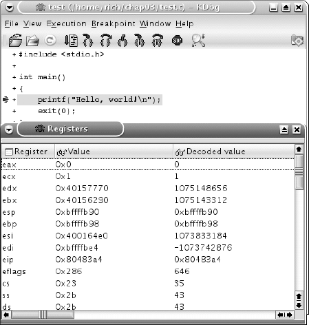
After the program files are loaded, and the desired view windows are set, you can start the program execution by clicking the run icon button. Just as in gdb, the program will execute until it reaches the first breakpoint. When it reaches the breakpoint, you can step through the program using the step icon button until the program finishes.

The objdump command-line parameters specify what functions the program will perform on the object code files, and how it will display the information it retrieves. The command-line format of objdump is as follows:

objdump [-a|--archive-headers] [-b bfdname|--target=bfdname]
        [-C|--demangle[=style] ] [-d|--disassemble]
        [-D|--disassemble-all] [-z|--disassemble-zeroes]
        [-EB|-EL|--endian={big | little }] [-f|--file-headers]
        [--file-start-context] [-g|--debugging]
        [-e|--debugging-tags] [-h|--section-headers|--headers]
        [-i|--info] [-j section|--section=section]
        [-l|--line-numbers] [-S|--source]
        [-m machine|--architecture=machine]
        [-M options|--disassembler-options=options]
        [-p|--private-headers] [-r|--reloc]
        [-R|--dynamic-reloc] [-s|--full-contents]
        [-G|--stabs] [-t|--syms] [-T|--dynamic-syms]
        [-x|--all-headers] [-w|--wide]
        [--start-address=address] [--stop-address=address]
        [--prefix-addresses] [--[no-]show-raw-insn]
        [--adjust-vma=offset] [-V|--version] [-H|--help]
        objfile...

The command-line parameters are described in the following table.

The objdump program is an extremely versatile tool to have available. It can decode many different types of binary files besides just object code files. For the assembly language programmer, the -d parameter is the most interesting, as it displays the disassembled object code file.

Using the sample C program, you can create an object file to dump by compiling the program with the -c option:

$ gcc -c ctest.c
$ objdump -d ctest.o

ctest.o:     file format elf32-i386

Disassembly of section .text:

00000000 <main>:
   0:   55                      push   %ebp
   1:   89 e5                   mov    %esp,%ebp
   3:   83 ec 08                sub    $0x8,%esp
   6:   83 ec 0c                sub    $0xc,%esp
   9:   68 00 00 00 00          push   $0x0
   e:   e8 fc ff ff ff          call   f <main+0xf>
  13:   83 c4 10                add    $0x10,%esp
  16:   83 ec 0c                sub    $0xc,%esp
  19:   6a 00                   push   $0x0
  1b:   e8 fc ff ff ff          call   1c <main+0x1c>
$

The disassembled object code file created by your system may differ from this example depending on the specific compiler and compiler version used. This example shows both the assembly language mnemonics created by the compiler and the corresponding instruction codes. You may notice, however, that the memory addresses referenced in the program are zeroed out. These values will not be determined until the linker links the application and prepares it for execution on the system. In this step of the process, however, you can easily see what instructions are used to perform the functions.

As with all the other tools, gprof is a command-line program that uses multiple parameters to control its behavior. The command-line format for gprof is as follows:

gprof [ -[abcDhilLsTvwxyz] ] [ -[ACeEfFJnNOpPqQZ][name] ]
      [ -I dirs ] [ -d[num] ] [ -k from/to ]
      [ -m min-count ] [ -t table-length ]
      [ --[no-]annotated-source[=name] ]
      [ --[no-]exec-counts[=name] ]
      [ --[no-]flat-profile[=name] ] [ --[no-]graph[=name] ]
      [ --[no-]time=name] [ --all-lines ] [ --brief ]
      [ --debug[=level] ] [ --function-ordering ]
      [ --file-ordering ] [ --directory-path=dirs ]
      [ --display-unused-functions ] [ --file-format=name ]
      [ --file-info ] [ --help ] [ --line ] [ --min-count=n ]
      [ --no-static ] [ --print-path ] [ --separate-files ]
      [ --static-call-graph ] [ --sum ] [ --table-length=len ]
      [ --traditional ] [ --version ] [ --width=n ]
      [ --ignore-non-functions ] [ --demangle[=STYLE] ]
      [ --no-demangle ] [ image-file ] [ profile-file ... ]

This alphabet soup of parameters is split into three groups:

The output format options, described in the following table, enable you to modify the output produced by gprof.

The analysis parameters, described in the following table, modify the way gprof analyzes the data contained in the analysis file.

Finally, the miscellaneous parameters, described in the following table, are parameters that modify the behavior of gprof, but don't fit into either the output or analysis groups.

In order to use gprof on an application, you must ensure that the functions you want to monitor are compiled using the -pg parameter. This parameter compiles the source code, inserting a call to the mcount subroutine for each function in the program. When the application is run, the mcount subroutine creates a call graph profile file, called gmon.out, which contains timing information for each function in the application.

After the program to test finishes, the gprof program is used to examine the call graph profile file to analyze the time spent in each function. The gprof output contains three reports:

By default, the gprof output is directed to the standard output of the console. You must redirect it to a file if you want to save it.

To demonstrate the gprof program, you must have a high-level language program that uses functions to perform actions. I created the following simple demonstration program in C, called demo.c, to demonstrate the basics of gprof:

#include <stdio.h>

void function1()
{
        int i, j;
        for(i=0; i <100000; i++)
                j += i;
}
void function2()
{
        int i, j;
        function1();
        for(i=0; i < 200000; i++)
                j = i;
}

int main()
{
        int i, j;
        for (i = 0; i <100; i++)
                function1();

        for(i = 0; i<50000; i++)
                function2();
        return 0;
}

This is about as simple as it gets. The main program has two loops: one that calls function1() 100 times, and one that calls function2() 50,000 times. Each of the functions just performs simple loops, although function2() also calls function1() every time it is called.

The next step is to compile the program using the -pg parameter for gprof. After that the program can be run:

$ gcc -o demo demo.c -pg
$ ./demo
$

When the program finishes, the gmon.out call graph profile file is created in the same directory. You can then run the gprof program against the demo program, and save the output to a file:

$ ls -al gmon.out
-rw-r--r--    1 rich     rich          426 Jul  7 12:39 gmon.out
$ gprof demo > gprof.txt
$

Notice that the gmon.out file was not referenced in the command line, just the name of the executable program. gprof automatically uses the gmon.out file located in the same directory. This example redirected the gprof output to a file named gprof.txt. The resulting file contains the complete gprof report for the program. Here's what the flat profile section looked like on my system:

%   cumulative   self              self     total
 time   seconds   seconds    calls  us/call  us/call  name
 67.17    168.81   168.81    50000  3376.20  5023.11  function2
 32.83    251.32    82.51    50100  1646.91  1646.91  function1

This report shows the total processor time and times called for each individual function that was called by main. As expected, function2 took the majority of the processing time.

The next report is the call graph, which shows the breakdown of time by individual functions, and how the functions were called:

index % time    self  children    called     name
                                                 <spontaneous>
[1]    100.0    0.00  251.32                 main [1]
              168.81   82.35   50000/50000       function2 [2]
                0.16    0.00     100/50100       function1 [3]
-----------------------------------------------
              168.81   82.35   50000/50000       main [1]
[2]     99.9  168.81   82.35   50000         function2 [2]
               82.35    0.00   50000/50100       function1 [3]
-----------------------------------------------
                0.16    0.00     100/50100       main [1]
               82.35    0.00   50000/50100       function2 [2]
[3]     32.8   82.51    0.00   50100         function1 [3]
-----------------------------------------------

Each section of the call graph shows the function analyzed (the one on the line with the index number), the functions that called it, and its child functions. This output is used to track the flow of time throughout the program.

If you are new to the Linux environment, you may need some background information before trying out a Linux distribution. When people talk about the Linux operating system, they are really talking about an entire suite of programs, not all of them necessarily related to Linux. The key to building a Linux system is understanding the components that comprise the system, and knowing where and how to get them.

Linus Torvalds is credited with creating and guiding the development of the Linux operating system kernel. The operating system kernel is the software that interacts with the hardware and handles the low-level functions of an operating system, such as file access control, and handling memory and hardware interfaces. Just loading a Linux kernel on a computer would be a pretty boring experience. You need additional programs to interact with the devices to really do anything.

This is where the GNU project comes in. The GNU project has developed many applications over the years that help system administrators and programmers with any UNIX-type operating system, with Linux being one of the more popular.

When you download a Linux distribution, what you are downloading is the Linux kernel, bundled with a set of utilities to perform the desired functions for the type of system you want to build. Most of the standard UNIX functions have been implemented by the GNU project. Depending on what you want your particular Linux system do to, you may or may not want to install all of the available GNU programs.

After you build your base Linux system, you will want to create your specific development environment. When you decide which tools you want to include on your system, first check to see if they are available on the distribution disks included with the Linux distribution. This is by far the easiest way to install packages, especially if you are using a distribution that includes an automated package manager, such as Red Hat rpm or Debian dpkg.

If you do not (or cannot) install a complete Linux system, the next best thing is to use a bootable CD distribution. With a bootable CD distribution, the entire Linux system is stored on a bootable CD. To run Linux, just place the CD in your computer and reboot. The Linux system will load in memory, and create a virtual disk in memory. The operating system on the hard drive is never touched. When you are finished, just take the CD out and reboot from the hard drive. Most bootable Linux CD distributions do an excellent job of auto-detecting workstation hardware, such as network cards, sound cards, and various graphics cards.

One of my favorite bootable Linux CD distributions for development is MEPIS Linux. The MEPIS Linux distribution is based on the Debian Linux, but comes as a bootable CD that can also be easily installed on your hard drive if you choose to do so. It is one of the easiest ways to install Linux on an existing workstation system.

Another reason MEPIS is one of my favorites is that, at the time of this writing, the MEPIS bootable CD contains a complete development environment, including gas, ld, gcc, gdb, gprof, and even kdbg. By just booting from the MEPIS CD, you have an automatic Linux assembly language development system!

The following sections describe how to download and use the MEPIS Linux distribution.

The MEPIS Web site is located at www.mepis.org. From that page, you can purchase a CD, buy a premium download subscription, or go to a free download mirror site. At the time of this writing, the current full release version of MEPIS is 2003-10, patch 2, and the current beta version is 2004-b05.

The full version MEPIS CD is downloaded as two separate .iso format files:

If you plan on downloading the distribution files, you might want to find a high-speed Internet connection, as the file is 694MB in size. After downloading the .iso files, you must have a workstation with a CD burner, and software that allows burning CDs from .iso files. After burning the .iso files to CDs, you are ready to start MEPIS Linux.

The first .iso file contains the complete operating system that can be run from the CD. First ensure that your workstation allows booting from CDs (an option that is set in the system BIOS). When you boot from the MEPIS Linux CD, a boot screen appears, asking for any special boot parameters. In most cases, you can simply press Enter to continue the boot process. If you have a video card that is not supported by MEPIS, you can enter boot prompt parameters. See the MEPIS Web site for specific details.

After the system boots, the KDE desktop login screen appears, with two preconfigured user IDs, demo and root. You can log in as either account, but it is safest to use the demo account. The password for demo is demo, and the password for root is root.

When you log into the MEPIS system, you will see the KDE desktop environment displayed. This is similar to a Microsoft Windows desktop environment, with desktop icons, a taskbar, and a Start button (although it is not called Start on the KDE desktop). You can open a command prompt session by clicking the shell icon on the taskbar. You can also open an editor session using any one of several different editors from the Editors menu item.

After creating your assembly language program text file, you can use the as and ld commands from a command prompt session to assemble and link the program. If you are creating high-level language programs, MEPIS also includes the gcc compiler for C and C++ applications.

When it is time for debugging, MEPIS includes the gdb and kdbg programs. The gdb program can be accessed from a command prompt session, while the kdbg program is available on the menu under the Development section.

The only drawback to running a development system from a bootable CD is when it is time to save your work. By default, the system uses RAM memory as a virtual disk. Any program stored under the default file system is only stored in memory. The next time you boot from the CD, the files will be gone.

To solve this problem, you should have some type of media available that MEPIS can access. Unfortunately, at the time of this writing, MEPIS is unable to write data to hard drives using the NTFS format (commonly used in Windows 2000 and XP workstations). If you have a hard drive formatted using the FAT32 format, MEPIS will be able to write to there. Also, MEPIS can write files to a floppy disk, and to most USB flash drives. As a last resort, if your workstation is on a local area network (LAN), you can always copy the files over by either using the FTP protocol or mounting a Windows shared drive to the system. My favorite method is to use a Windows share on a separate computer. It's just as simple as mapping in the Windows world.