
After you start coding various types of utilities for different projects, you will realize that you are coding the same utilities multiple times within the same program, or possibly using the same utilities within different programs. Instead of having to retype the code for the utility every time you need to use it, you can create a standalone function that can be called anytime you need the utility.
This chapter describes what functions are and how they are used in programs. You will learn how functions are used in assembly language, including examples of how they are created and used in assembly language programs. After that, you will learn how to create assembly language functions using the C calling convention, as well as how to split assembly language functions into files separate from the main program. Finally, because passing parameters is important to functions as well as programs, you will learn how to read and process command-line parameters from within an assembly language program, and examine a demonstration of how to use command-line parameters in your application.
Often, applications require that the same procedures or processes be performed multiple times with different data sets. When the same code is required throughout an application, instead of rewriting the code multiple times, it is sometimes best to create a single function containing the code, which can then be called from anywhere in the program. A function contains all of the code necessary to complete a specific routine, without requiring any code assistance from the main program. Data is passed to the function from the main program, and the results are returned back to the main program.
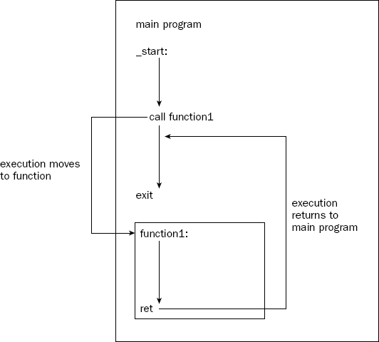
When a function is called, the execution path of the program is altered, switching to the first instruction in the function code. The processor executes instructions from that point, until the function indicates that it can return control back to the original location in the main program. This is demonstrated in Figure 11-1.
Most high-level languages provide a method to write and use functions within programs. Functions can be contained and compiled in the same source code file as the main program, or they can be located in a separate source code file and be linked with the main program.
The ctest.c program demonstrates a simple C language function that calculates the area of a circle given the radius:
/* ctest.c - An example of using functions in C */
#include <stdio.h>

float function1(int radius)
{
   float result = radius * radius * 3.14159;
   return result;
}

int main()
{
   int i;
   float result;
   i = 10;
   result = function1(i);
   printf("Radius: %d,  Area: %f
", i, result);
i = 2;
result = function1(i);
printf("Radius: %d, Area: %f
", i, result);
i = 120;
result = function1(i);
printf("Radius: %d, Area: %f
", i, result);
return 0;
}The function defines the required input value, as well as the type of output the function will produce:
float function1(int radius)
The function definition shows that the input value is an integer, and the function produces a floating-point value for the output. When the function is called within the program, it must use the same format:
result = function1(i);
The variable placed inside the function call is defined as an integer, and the output of the function is stored in the variable result, which is defined as a floating-point value. To compile the program, you can use the GNU C compiler (gcc):
$ gcc -o ctest ctest.c
$./ctest
Radius: 10,  Area: 314.158997
Radius: 2,  Area: 12.566360
Radius: 120,  Area: 45238.894531
$
Now that you have seen how functions work in general, it's time to create some functions in assembly language.
Writing functions in assembly language is similar to writing them with C. To create a function, you must define its input values, how it processes the input values, and its output values. Once the function is defined, you can code it within your assembly language application.
This section shows how to create functions in assembly language programs, and provides a simple example of using a function within a program.
Three steps are required for creating functions in assembly language programs:
This section walks through these steps using the area of a circle function as an example.
Many (if not most) functions require some sort of input data. You must decide how your program will pass this information along to the function. Basically, three techniques can be employed:
Using registers
Using global variables
Using the stack
The simple example shown in this section uses the registers technique to pass an input value to the function. The second two techniques, global variables and the stack, are covered in detail later in this chapter.
When functions are called from the main program, they pick up execution from where the main program left off when the function was called. Any data located in memory and in the registers is fair game to the function. Using the registers to pass input values to a function is quick and simple.
When using registers to pass data between the main program and functions, remember to use the proper data type for the data. The data must be placed in the register in the same data type that the function expects.
The function is written as normal assembly language code within the program. The function instructions must be set apart from the rest of the main program instructions in the source code file.
What makes the function different from the rest of the main program is the way it is defined for the assembler. Different assemblers use different methods for defining functions.
To define a function in the GNU assembler, you must declare the name of the function as a label in the program. To declare the function name for the assembler, use the .type directive:
.type func1, @function
func1:
The .type directive informs the GNU assembler that the func1 label defines the start of a function that will be used within the assembly language program. The func1 label defines the start of the function. The first instruction after the func1 label is the beginning of the function.
Within the function, code can be used just as with the main program code. Registers and memory locations can be accessed, and special features such as the FPU, MMX, and SSE can be utilized.
The end of the function is defined by a RET instruction. When the RET instruction is reached, program control is returned to the main program, at the instruction immediately following where the function was called with the CALL instruction.
When the function finishes processing the data, most likely you will want to retrieve the result back in the calling program area. The function must have a way to pass the result back to the main program so the main program can utilize the data for further processing or displaying. Similar to the input value techniques, there are multiple ways to accomplish transferring results, although the following two are most popular:
Place the result in one or more registers.
Place the result in a global variable memory location.
The sample function used here uses a single register to pass the result back to the main program. Later in this chapter you will learn how to use the global variable techniques to pass data back to the main program.
Now that you have seen the basics for creating assembly language functions, it's time to create one. This code snippet shows how a function could be created to perform the area function in an assembly language program:
.type area, @function
area:
   fldpi
   imull %ebx, %ebx
   movl %ebx, value
   filds value
   fmulp %st(0), %st(1)

   ret
The area function uses the FPU to calculate the area of a circle, based on the radius. The input value (the radius) is assumed to be an integer value, located in the EBX register when the function is called.
The pi value needed for the calculation is loaded into the FPU register stack using the FLDPI instruction. Next, the value in the EBX register is squared and stored in a memory location already defined in memory by the main program (remember that the function has full access to the memory locations defined by the main program).
The FILDS instruction is used to load the squared radius value into the top of the FPU stack, moving the pi value to the ST(1) position. Next, the FMULP instruction is used to multiply the first and second FPU stack positions, placing the result in the ST(1) position, and then popping the ST(0) value off of the stack, leaving the final result in the ST(0) register.
The requirements for a program to use the area function are as follows:
The input value must be placed in the
EBXregister as an integer value.A 4-byte memory location called
valuemust be created in the main program.The output value is located in the
FPU ST(0)register.
It is crucial to follow these requirements when using the area function within the main program. For example, if you place the radius value in the EBX register as a floating-point data type, the entire area calculation will be incorrect.
The sample area function shown here has a complicated set of requirements that must be followed in order for an application to use it. If you are working with a large application with numerous functions, it would be difficult to keep track of which functions had which sets of requirements. There is a way to remedy this, which is demonstrated in the section "Passing Data Values in C Style."
Once the function is created, it can be accessed from anywhere in the program. The CALL instruction is used to pass control from the main program to the function. The CALL instruction has a single operand:
call function
where function is the name of the function to call. Remember to place any input values in the appropriate locations before the CALL instruction.
The functest1.s program demonstrates performing multiple calls to the area function within a program:
# functest1.s - An example of using functions
.section .data
precision:
   .byte 0x7f, 0x00
.section .bss
   .lcomm value, 4
.section .text
.globl _start
_start:
   nop
   finit
   fldcw precision

   movl $10, %ebx
   call area

   movl $2, %ebx
   call area

   movl $120, %ebx
   call area

   movl $1, %eax
   movl $0, %ebx
   int $0x80

.type area, @function
area:
   fldpi
   imull %ebx, %ebx
   movl %ebx, value
filds value
   fmulp %st(0), %st(1)
   fstps %eax
   ret
The area function is created exactly as the code snippet earlier demonstrated. The main program first initializes the FPU and sets it to use single-precision floating-point results (See Chapter 9, "Advanced Math Functions"). Next, three calls are made to the area function, each time using a different value in the EBX register. The output from the function is placed in the EAX register as a single-precision floating-point data type. For this example, the results are not displayed. Instead, they can be viewed from the debugger while running the program.
After assembling and linking the program, run it in the debugger, and watch how the program execution moves. When the CALL instruction is performed, the next instruction executed is the first instruction in the function:
$ gdb -q functest1
(gdb) break *_start+1
Breakpoint 1 at 0x8048075: file functest1.s, line 11.
(gdb) run
Starting program: /home/rich/palp/chap11/functest1

Breakpoint 1, _start () at functest1.s:11
11         finit
Current language:  auto; currently asm
(gdb) s
12         fldcw precision
(gdb) s
14         movl $10, %ebx
(gdb) s
15         call area
(gdb) s
29         fldpi
(gdb)
Continuing to step through the program, the next instruction in the function is performed, and so on until the RET instruction, which returns to the main program:
(gdb) s
37         ret
(gdb) s
17         movl $2, %ebx
(gdb)
After returning to the main program, you can view the result value in the ST(0) register as a floating-point value:
(gdb) print/f $st0
$1 = 314.159271
(gdb)
The function performed as expected, producing the correct area value for the first radius value (10). This process continues for the other values and function calls.
You may have noticed that in the functest1.s program, the function code was placed after the end of the source code for the main program. You can also place the function code before the source code for the main program. As mentioned in Chapter 4, "A Sample Assembly Language Program," when the source code object file is linked, the linker is looking for the code section labeled _start for the first instruction to execute. You can have any number of functions coded before the _start label without affecting the start of the main program.
In addition, as demonstrated in the functest1.s program, unlike some high-level languages, the functions do not have to be defined before they are called in the main program. All the CALL instruction is looking for is the label to define where the function begins for the instruction pointer.
While the area function used only a single output register in the process, that may not be the case with more complex functions. Often functions use registers for processing data. There is no guarantee that the registers will be in the same state when the function is finished as they were before the function was called.
When calling a function from a program, you should know what registers the function uses for its internal processing. Any registers (and memory locations as well) used within the function may or may not be the same values when execution returns to the main program.
If you are calling a function that modifies registers the main program uses, it is crucial that you save the current state of the registers before calling the function, and then restore them after the function returns. You can either save specific registers individually using the PUSH instruction or save all of the registers together using the PUSHA instruction before calling the function. Similarly, you can restore the registers back to their original state either individually using the POP instruction or together using the POPA instruction.
Be careful when restoring the register values after the function call. If the function returns a value in a register, you must move it to a safe place before restoring the original register values.
You have already seen in the sample area function that functions can access memory locations defined in the main program. Because these memory locations are accessible by all of the functions in the program, they are called global variables. Functions can use global variables for any purpose, including passing data between the main program and the functions.
The functest2.s program demonstrates using global variables to pass input and output values between the function and the main program:
# functest2.s - An example of using global variables in functions
.section .data
precision:
   .byte 0x7f, 0x00
.section .bss
   .lcomm radius, 4
   .lcomm result, 4
.lcomm trash, 4
.section .text
.globl _start
_start:
   nop
   finit
   fldcw precision

   movl $10, radius
   call area

   movl $2, radius
   call area

   movl $120, radius
   call area

   movl $1, %eax
   movl $0, %ebx
   int $0x80

.type area, @function
area:
   fldpi
   filds radius
   fmul %st(0), %st(0)
   fmulp %st(0), %st(1)
   fstps result

   ret
The functest2.s program modifies the area function so that it does not need to use any general-purpose registers. Instead, it takes the input value from the radius global variable, loads it into the FPU, performs all of the mathematical operations within the FPU, and then pops the FPU ST(0) register into a global variable that can be accessed by the main program. Because no registers are used to hold input values, the main program must load each input value into the radius global variable instead of a register.
After assembling and linking the program, you can run it in the debugger to watch the global variables as the program progresses. Here are the values after the first call to the area function:
(gdb) x/d &radius
0x80490d4 <radius>:     10
(gdb) x/f &result
0x80490d8 <result>:     314.159271
(gdb)
The result was properly placed in the result memory location. After the first call to the function, a new value is loaded into the radius memory location, and the function is called again. This continues with the third call as well.
Using global memory locations to pass parameters and return results is not a common programming practice, even in C and C++ programming. The next section describes the more common method of passing values between functions.
As you can tell, numerous options are available for handling input and output values in functions. While this might seem like a good thing, in reality it can become a problem. If you are writing functions for a large project, the documentation required to ensure that each function is used properly can become overwhelming. Trying to keep track of which function uses which registers and global variables, or which registers and global variables are used to pass which parameters, can be a nightmare.
To help solve this problem, a standard must be used to consistently place input parameters for functions to retrieve, and consistently place output values for the main program to retrieve. When creating code for the IA-32 platform, most C compilers use a standard method for handling input and output values in assembly language code compiled from C functions. This method works equally as well for any assembly language program, even if it wasn't derived from a C program.
The C solution for passing input values to functions is to use the stack. The stack is accessible from the main program as well as from any functions used within the program. This creates a clean way to pass data between the main program and the functions in a common location, without having to worry about clobbering registers or defining global variables.
Likewise, the C style defines a common method for returning values to the main program, using the EAX register for 32-bit results (such as short integers), the EDX:EAX register pair for 64-bit integer values, and the FPU ST(0) register for floating-point values.
The following sections review how the stack works and show how it is used to pass input values to functions.
The basic operation of the stack was discussed briefly in Chapter 5, "Moving Data." The stack consists of memory locations reserved at the end of the memory area allocated to the program. The ESP register is used to point to the top of the stack in memory. Data can be placed only on the top of the stack, and it can be removed only from the top of the stack.
Data is usually placed on the stack using the PUSH instruction. This places the data on the bottom of the memory area reserved for the stack and decreases the value in the stack pointer (the ESP register) to the location of the new data.
To retrieve data from the stack, the POP instruction is used. This moves the data to a register or memory location and increases the ESP register value to point to the previous stack data value.
Before a function call is made, the main program places the required input parameters for the function on the top of the stack. Of course, the programmer must know the order in which the function is expecting the data values to be placed on the stack, but that is usually part of the function documentation. The C style requires placing parameters on the stack in reverse order from the prototype for the function.
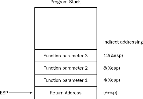
When the CALL instruction is executed, it places the return address from the calling program onto the top of the stack as well, so the function knows where to return. This leaves the stack in the state shown in Figure 11-2.

The stack pointer (ESP) points to the top of the stack, where the return address is located. All of the input parameters for the function are located "underneath" the return address on the stack. Popping values off of the stack to retrieve the input parameters would cause a problem, as the return address might be lost in the process. Instead, a different method is used to retrieve the input parameters from the stack.
Chapter 5 discussed the topic of indirect addressing using registers. This technique provides a method of accessing locations in memory based on the index value in a register. Because the ESP pointer points to the top of the stack (which contains the return address for the function), the function can use indirect addressing with the ESP register to access the input parameters without having to pop the values off of the stack. Figure 11-3 demonstrates this.
Each parameter can be indirectly accessed via the offset from the ESP register, without having to POP values off of the stack.
There is a problem with this technique, however. While in the function, it is possible that part of the function process will include pushing data onto the stack. If this happens, it would change the location of the ESP stack pointer and throw off the indirect addressing values for accessing the parameters in the stack.
To avoid this problem, it is common practice to copy the ESP register value to the EBP register when entering the function. This ensures that there is a register that always contains the correct pointer to the top of the stack when the function is called. Any data pushed onto the stack during the function would not affect the EBP register value. To avoid corrupting the original EBP register if it is used in the main program, before the ESP register value is copied, the EBP register value is also placed on the stack. This produces the scenario shown in Figure 11-4.
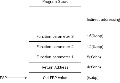
Now the EBP register contains the location of the start of the stack (which is now the old EBP register value). The first input parameter from the main program is located at the indirect addressing location 8(%ebp), the second parameter is located at the location 12(%ebp), and so on. These values can be used throughout the function without worrying about what other values are placed onto or taken off of the stack.
The technique of using the stack to reference input data for the function has created a standard set of instructions that are found in all functions written using the C function style technique. This code snippet demonstrates what instructions are used for the start and end of the function code:
function:
   pushl %ebp
   movl %esp, %ebp
   .
   .
   movl %ebp, %esp
   popl %ebp
   ret
The first two instructions at the top of the function code save the original value of EBP to the top of the stack, and then copy the current ESP stack pointer (now pointing to the original value of EBP in the stack) to the EBP register.
After the function processing completes, the last two instructions in the function retrieve the original value in the ESP register that was stored in the EBP register, and restore the original EBP register value. Resetting the ESP register value ensures that any data placed on the stack within the function but not cleaned off will be discarded when execution returns to the main program (otherwise, the RET instruction could return to the wrong memory location).
The ENTER and LEAVE instructions are specifically designed for setting up function prologues (the ENTER instruction) and epilogues (the LEAVE instruction). These can be used instead of creating the prologues by hand.
While the function code has control of the program, most likely the processes will need to store data elements someplace. As discussed earlier, registers can be used within the function code, but this provides a limited amount of work area. Global variables can also be used for working data, but this presents the problem of creating additional requirements for the main program to provide specific data elements for the function. When looking for an easy location for working storage for data elements within the function, the stack again comes to the rescue.
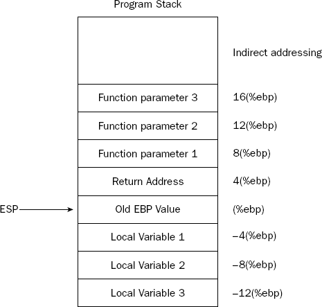
Once the EBP register is set to point to the top of the stack, any additional data used in the function can be placed on the stack after that point without affecting how the input values are accessed. This is shown in Figure 11-5.
Now that the local variables are defined on the stack, they can easily be referenced using the EBP register. Assuming 4-byte data values, the first local variable would be accessed by referencing −4(%ebp), while the second local variable would be accessed by referencing −8(%ebp).
There is still one lingering problem with this setup. If the function pushes any data onto the stack, the ESP register still points to the location before the local variables were placed and will overwrite those variables.
To solve this problem, at the start of the function code another line is added to reserve a set amount of stack space for local variables by subtracting the value from the ESP register. Figure 11-6 shows how this looks on the stack.
Now, if any data is pushed onto the stack, it will be placed beneath the local variables, preserving them so they can still be accessed via the EBP register pointer. The normal ESP register can still be used to push data onto the stack and pop it off of the stack without affecting the local variables.
When the end of the function is reached and the ESP register is set back to its original value, the local variables will be lost from the stack and will not be directly accessible using the ESP or EBP registers from the calling program (thus the term local variables).

The function prologue code now must include one additional line to reserve the space for the local variables by moving the stack pointer down. You must remember to reserve enough space for all of the local variables needed in the function. The new prologue would look like this:
function:
   pushl %ebp
   movl %esp, %ebp
   subl $8, %esp
   .
   .
This code reserves 8 bytes to be used for local variables. This space can be used as either two-word values or one doubleword value.
There is just one more detail to consider when using C style function calling. Before the function is called, the calling program places all of the required input values onto the stack. When the function returns, those values are still on the stack (since the function accessed them without popping them off of the stack). If the main program uses the stack for other things, most likely it will want to remove the old input values from the stack to get the stack back to where it was before the function call.
While you can use the POP instruction to do this, you can also just move the ESP stack pointer back to the original location before the function call. Adding back the size of the data elements pushed onto the stack using the ADD instruction does this.
For example, if you place two 4-byte integer values onto the stack and then call a function, you must add 8 to the ESP register to clean the data off of the stack:
pushl %eax
pushl %ebx
call compute
addl $8, %esp
This ensures that the stack is back to where it should be for the rest of the main program.
Now that you know how to use the stack for passing input values to functions, and for local variables within the functions, it's time for an example. The functest3.s program demonstrates how all of these components can work together to simplify the area function example:
# functest3.s - An example of using C style functions
.section .data
precision:
   .byte 0x7f, 0x00
.section .bss
   .lcomm result, 4
.section .text
.globl _start
_start:
   nop
   finit
   fldcw precision

   pushl $10
   call area
   addl $4, %esp
   movl %eax, result

   pushl $2
   call area
   addl $4, %esp
   movl %eax, result

   pushl $120
   call area
addl $4, %esp
   movl %eax, result

   movl $1, %eax
   movl $0, %ebx
   int $0x80

.type area, @function
area:
   pushl %ebp
   movl %esp, %ebp
   subl $4, %esp
   fldpi
   filds 8(%ebp)
   fmul %st(0), %st(0)
   fmulp %st(0), %st(1)
   fstps −4(%ebp)
   movl −4(%ebp), %eax

   movl %ebp, %esp
   popl %ebp
   ret
The area function code was modified to utilize the stack to retrieve the radius input value, and use a local function variable to move the result from the ST(0) register to the EAX register as a single-precision floating-point value. The result of the function is returned in the EAX register instead of the ST(0) register to help demonstrate using the local variable. In Chapter 14, "Calling Assembly Libraries," you will see that C programs expect the result in the ST(0) register.
After the standard function prologue (including reserving 4 bytes of space on the stack for a local variable), the pi value and the radius value are loaded into the FPU stack:
fdpi
filds 8(%ebp)
The 8(%ebp) value references the first parameter placed on the stack by the calling program. After the area result is calculated, it is placed in the local variable data:
fstps −4(%ebp)
The −4(%ebp) value references the first local variable on the stack. That value is placed into the EAX register, where it is retrieved by the main program.
Following that, the standard function epilogue instructions are used to replace the ESP and EBP pointer values and to return control back to the main program.
Notice the new code within the main program used for each radius value:
pushl $10
call area
addl $4, %esp
movl %eax, result
Each radius value is pushed onto the stack before the call to the area function. When the function completes, the stack is reset to its previous location by adding 4 (the data size of the radius value) to the ESP register. The result is then moved from the EAX register to the global variable memory location.
You can watch how all of the data values are placed in the stack area while the program is running by using the debugger. After assembling and linking the program, run the program in the debugger, set a breakpoint at the start of the program, and look at where the stack pointer is set:
$ gdb -q functest3
(gdb) break *_start+1
Breakpoint 1 at 0x8048075: file functest3.s, line 11.
(gdb) run
Starting program: /home/rich/palp/chap11/functest3

Breakpoint 1, _start () at functest3.s:11
11         finit
Current language:  auto; currently asm
(gdb) print $esp
$1 = (void *) 0xbffff950
(gdb)
The stack point is currently set to the memory address at 0xbffff950. Step through the program until after the first PUSHL instruction before the CALL instruction, and look at the stack pointer value and the value of the data element in the last stack position:
(gdb) s
14         pushl $10
(gdb) s
15         call area
(gdb) print $esp
$2 = (void *) 0xbffff94c
(gdb) x/d 0xbffff94c
0xbffff94c:     10
(gdb)
After the PUSHL instruction, the new stack pointer value is 4 bytes less than the original (as expected). The data value pushed onto the stack is now shown at that memory location. Now, step through the CALL instruction, and again examine the stack:
(gdb) s
35         pushl %ebp
(gdb) print $esp
$3 = (void *) 0xbffff948
(gdb) x/x 0xbffff948
0xbffff948:     0x08048085
(gdb) x/d 0xbffff94c
0xbffff94c:     10
(gdb)
Again, the value of the ESP register is decreased, and the value stored there is the memory location of the instruction immediately following the CALL instruction. The input parameter is still located in the next stack position.
Control of the program is now in the area function. After stepping through the PUSHL instruction, the ESP register is again decreased, with the original value of EBP placed in the stack:
(gdb) s
36         movl %esp, %ebp
(gdb) print $esp
$5 = (void *) 0xbffff944
 (gdb) x/x 0xbffff944
0xbffff944:     0x00000000
(gdb)
Stepping through one more step in the instructions loads the ESP register value into EBP, which can now be used in indirect addressing to access the data on the stack. You can see the three values stored in the stack using the debugger:
(gdb) x/3x ($ebp)
0xbffff944:     0x00000000      0x08048085      0x0000000a
(gdb)
The stack now contains the original value of EBP, the return address from the CALL instruction, and the input value placed on the stack with the PUSH instruction.
Next, the ESP register is decreased to make room for the local variable:
(gdb) s
area () at functest3.s:37
37         subl $4, %esp
(gdb) s
38         fldpi
(gdb) print $esp
$1 = (void *) 0xbffff940
(gdb)
The new ESP location is 0xbffff940, while the EBP value is 0xbffff944. This leaves 4 bytes for a 32-bit single-precision floating-point value to be stored.
The pi value, as well as the input parameter, are loaded into the FPU stack, which can be examined using the info all command in the debugger:
(gdb) info all
.
.
st0   10      (raw 0x4002a000000000000000)
st1   3.1415926535897932385128089594061862 (raw 0x4000c90fdaa22168c235)
(gdb)
The input parameter was successfully loaded into the FPU stack using the FILDS instruction.
Stepping through the rest of the area function instructions, you can stop when the result is placed in the local variable on the stack, and see what happens:
(gdb) s
42         fstps −4(%ebp)
(gdb) s
43         movl −4(%ebp), %eax
(gdb) x/4x 0xbffff940
0xbffff940:     0x439d1463      0x00000000      0x08048085      0x0000000a
(gdb) x/f 0xbffff940
0xbffff940:     314.159271
(gdb)
The result value was placed into the stack at the −4(%ebp) location. It can be viewed in the debugger by reading the memory location and setting the output to floating-point format using the x/f command.
The last steps in the function reset the ESP and EBP registers back to their original values:
(gdb) s
45         movl %ebp, %esp
(gdb) s
46         popl %ebp
(gdb) print $esp
$2 = (void *) 0xbffff944
(gdb) print $ebp
$3 = (void *) 0xbffff944
(gdb) s
area () at functest3.s:47
47         ret
(gdb) print $esp
$4 = (void *) 0xbffff948
(gdb) print $ebp
$5 = (void *) 0x0
(gdb)
Now the ESP register points to the return location for the CALL instruction. When the RET instruction is executed, program control returns to the main program:
(gdb) s
area () at functest3.s:47
47         ret
(gdb) print $esp
$4 = (void *) 0xbffff948
(gdb) print $ebp
$5 = (void *) 0x0
(gdb) s
16         addl $4, %esp
(gdb) s
17         movl %eax, result
(gdb) print $esp
$6 = (void *) 0xbffff950
(gdb)
When control is returned, the ESP value is then increased by four to remove the radius value pushed onto the stack. The new stack pointer value is now 0xbffff950, which is where it was at the start of things. The process is ready to be started all over again with the next radius value.
Another benefit of using C style function calls is that the function is completely self-contained. No global memory locations need to be defined for accessing data, so .data directives do not need to be included in the functions.
This freedom creates another benefit: You no longer need to include the function source code in the same file as the main program source code. For programmers working on large projects that involve multiple people, this is a great benefit. Individual functions can be self-contained in their own files, and linked together for the final product. With code functions contained in separate files, you can see how it can quickly become a problem to continue using global variables to pass data around. Each function file would need to keep track of the global variables used.
This section demonstrates how to create separate function files, and how to assemble and link them with the main program file.
The self-contained function file is similar to the main program files you are used to creating. The only difference is that instead of the _start section, you must declare the function name as a global label, so other programs can access it. This is done using the .globl directive:
.section .text
.type area, @function
.globl area
area:
The preceding code snippet defines the global label area, which is the start of the area function used earlier. The .type directive is used to declare that the area label points to the start of a function. The complete function is shown in the file area.s:
# area.s - The area function
.section .text
.type area, @function
.globl area
area:
   pushl %ebp
   movl %esp, %ebp
   subl $4, %esp
   fldpi
   filds 8(%ebp)
   fmul %st(0), %st(0)
   fmulp %st(0), %st(1)
   fstps −4(%ebp)
   movl −4(%ebp), %eax
movl %ebp, %esp
   popl %ebp
   ret
The area.s file contains the complete source code for the area function, as shown in the functest3.s program. This version uses the C style function calls, so the input value is taken from the stack, which is also used for defining a local variable. The area function uses the EAX register to return the output result.
Finally, the main program must be created, using the normal format for calling the external functions. This is shown in the functest4.s program:
# functest4.s - An example of using external functions
.section .data
precision:
   .byte 0x7f, 0x00
.section .bss
   .lcomm result, 4
.section .text
.globl _start
_start:
   nop
   finit
   fldcw precision

   pushl $10
   call area
   addl $4, %esp
   movl %eax, result

   pushl $2
   call area
   addl $4, %esp
   movl %eax, result

   pushl $120
   call area
   addl $4, %esp
   movl %eax, result

   movl $1, %eax
   movl $0, %ebx
   int $0x80
Because none of the code required for the area function is contained in the main program, the main program listing becomes shorter and less cluttered.
Once the function and main program files are created, they must be assembled and linked together. Each program file must be assembled separately, which creates an object file for each file:
$ as -gstabs -o area.o area.s
$ as -gstabs -o functest4.o functest4.s
$
Now there are two object files that are required to be linked together to create the executable file. If you do not link the function object file, the linker will produce an error:
$ ld -o functest4 functest4.o
functest4.o:functest4.s:15: undefined reference to 'area'
functest4.o:functest4.s:20: undefined reference to 'area'
functest4.o:functest4.s:25: undefined reference to 'area'
$
The linker could not resolve the calls to the area function. To create the executable program, you must include both object files in the linker command line:
$ ld -o functest4 functest4.o area.o
$
The program can now be run in the debugger as before, with the same results.
You may have noticed that when both the function file and the main program file were assembled, I used the -gstabs command-line option. This ensured that both the function and the main program could be viewed in the debugger. Sometimes, when working on large programs that contain numerous long functions, this is not desired.
Instead of having to step through long functions several times before reaching the function you want to debug, you can choose to not debug individual function files. Instead of using the -gstabs option when assembling all of the functions, use it for only the function you want to debug, along with the main program.
For example, you can assemble the area.s function without the -gstabs option, and then watch what happens when you step through the functest4 program:
$ as -o area.o area.s
$ as -gstabs -o functest3.o functest4.s
$ ld -o functest4 functest4.o area.o
$ gdb -q functest4
(gdb) break *_start+1
Breakpoint 1 at 0x8048075: file functest4.s, line 11.
(gdb) run
Starting program: /home/rich/palp/chap11/functest4

Breakpoint 1, _start () at functest4.s:11
11         finit
Current language:  auto; currently asm
(gdb) s
12         fldcw precision
(gdb) s
14         pushl $10
(gdb) s
15         call area
(gdb) s
0x080480b8      31         int $0x80
(gdb) s
16         addl $4, %esp
(gdb)
When stepping through the main program, when the CALL instruction is executed, it is treated as a single instruction, and the next instruction in the debugger is the next instruction in the main program. All of the instructions in the area function were processed without stopping. To see that it worked properly, you can check the return values to verify that the function worked:
(gdb) print/f $eax
$1 = 314.159271
(gdb)
Indeed, the EAX register contains the result from the first call to the area function.
Related to the topic of passing parameters to functions is the topic of passing parameters to programs. Some applications require input parameters to be specified on the command line when the program is started. This section describes how you can utilize this feature in your assembly language programs.
Different operating systems use different methods for passing command-line parameters to programs. Before trying to explain how command-line parameters are passed to programs in Linux, it's best to first explain how Linux executes programs from the command line in the first place.
When a program is run from a Linux shell prompt, the Linux system creates an area in memory for the program to operate. The memory area assigned to the program can be located anywhere on the system's physical memory. To simplify things, each program is assigned the same virtual memory addresses. The virtual memory addresses are mapped to physical memory addresses by the operating system.
The virtual memory addresses assigned to programs running in Linux start at address 0x8048000 and end at address 0xbfffffff. The Linux OS places the program within the virtual memory address area in a specific format, shown in Figure 11-7.
The first block in the memory area contains all the instructions and data (from both the .bss and .data sections) of the assembly program. The instructions include not only the instruction codes from your assembly program, but also the necessary instruction information from the linking process for Linux to run the program.
The second block in the memory area is the program stack. As mentioned in Chapter 2, "The IA-32 Platform," the stack grows downward from the end of the memory area. Given this information, you would expect the stack pointer to be set to 0xbfffffff each time a program starts, but this is not the case. Before the program loads, Linux places a few things into the stack, which is where the command-line parameters come in.

Linux places four types of information into the program stack when the program starts:
The program name, command-line parameters, and environment variables are variable-length strings that are null terminated. To make your life a little easier, Linux not only loads the strings into the stack, it also loads pointers to each of these elements into the stack, so you can easily locate them in your program.
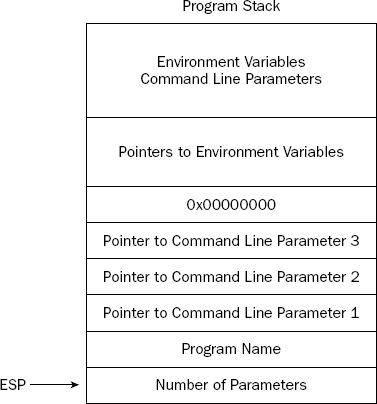
The layout of the stack when a program starts generally looks like what is shown in Figure 11-8.
Starting at the stack pointer (ESP), the number of command-line parameters used to start the program is specified as a 4-byte unsigned integer value. Following that, the 4-byte pointer to the program name location is placed in the next location in the stack. After that, pointers to each of the command-line parameters are placed in the stack (again, each 4 bytes in length).
You can use the debugger to see how this works. Run the functest4 program (presented earlier in the section "Creating a separate function file") in the debugger, and watch the stack when the program starts. First, start the program, and give it a command-line parameter (this is done in the run command in the debugger):
$ gdb -q functest4
(gdb) break *_start+1
Breakpoint 1 at 0x8048075: file functest4.s, line 11.
(gdb) run 10
Starting program: /home/rich/palp/chap11/functest4 10

Breakpoint 1, _start () at functest4.s:11
11         finit
Current language:  auto; currently asm
(gdb) print $esp
$1 = (void *) 0xbffff950
(gdb)
Notice that the Starting program line indicates the command-line parameter specified in the run command. The ESP pointer shows that it is pointing to memory location 0xbffff950. This indicates the top of the stack. You can view the values there using the x command:
(gdb) x/20x 0xbffff950
0xbffff950:  0x00000002   0xbffffa36   0xbffffa57   0x00000000
0xbffff960:  0xbffffa5a   0xbffffa75   0xbffffa95   0xbffffaa7
0xbffff970:  0xbffffabf   0xbffffadf   0xbffffaf2   0xbffffb14
0xbffff980:  0xbffffb26   0xbffffb38   0xbffffb41   0xbffffb4b
0xbffff990:  0xbffffd29   0xbffffd37   0xbffffd58   0xbffffd72
(gdb)
The x/20x command displays the first 20 bytes starting at the specified memory location, in hexadecimal format. The first value indicates the number of command-line parameters (including the program name). The next two memory locations contain pointers to the program name and command-line parameter strings as stored later in the stack. You can view the string values using the x command and the pointer address:
(gdb) x/s 0xbffffa36
0xbffffa36:      "/home/rich/palp/chap11/functest4"
(gdb) x/s 0xbffffa57
0xbffffa57:      "10"
(gdb)
As expected, the first pointer pointed to the program name string stored in the stack area. The second pointer pointed to the string for the command-line parameter.
Be careful: It is important to remember that all command-line parameters are specified as strings, even if they look like numbers.
After the command-line parameters, a 4-byte null value is placed on the stack to separate them from the start of the pointers to the environment variables. Again, you can use the x command to view some of the environment variables stored on the stack:
(gdb) x/s 0xbffffa5a
0xbffffa5a:      "PWD=/home/rich/palp/chap11"
(gdb) x/s 0xbffffa75
0xbffffa75:      "http_proxy=http://webproxy:1234"
(gdb) x/s 0xbffffa95
0xbffffa95:      "LC_MESSAGES=en_US"
(gdb) x/s 0xbffffaa7
0xbffffaa7:      "HOSTNAME=test1.blum.lan"
(gdb) x/s 0xbffffabf
0xbffffabf:      "NLSPATH=/usr/share/locale/%l/%N"
(gdb) x/s 0xbffffadf
0xbffffadf:      "LESSKEY=/etc/.less"
(gdb)
Depending on what applications you have loaded on your Linux box, numerous environment variables may be loaded here.
Now that you know where the command-line parameters are located on the stack, it is easy to write a simple program to access them and list them. The paramtest1.s program does just that.
# paramtest1.s - Listing command line parameters
.section .data
output1:
   .asciz "There are %d parameters:
"
output2:
   .asciz "%s
"
.section .text
.globl _start
_start:
   movl (%esp), %ecx
   pushl %ecx
   pushl $output1
   call printf
   addl $4, %esp
   popl %ecx
   movl %esp, %ebp
   addl $4, %ebp
loop1:
   pushl %ecx
   pushl (%ebp)
   pushl $output2
   call printf
   addl $8, %esp
   popl %ecx
   addl $4, %ebp
   loop loop1
   pushl $0
   call exit
The paramtest1.s program first reads the number of command-line parameter values from the top of the stack and places the value in the ECX register (so it can be used as a loop value). After that, it pushed the value onto the stack, along with the output text string for the printf C library function to display.
After the call to the printf function, you must clean the pushed values off of the stack. In this case, however, it works to our advantage, as we need to restore the ECX value after the printf function destroyed it. Next, the stack pointer in the ESP register is copied to the EBP pointer, so we can walk through the values without destroying the stack pointer. The EBP pointer is incremented by four to skip over the command-line parameter count value, ready to read the first parameter.
In the loop, first the current value of ECX is pushed onto the stack so it can be restored after the printf function. Next, the pointer to the first command-line parameter string (located in the memory address pointed to by the EBP register) is pushed onto the stack, along with the output string to display it for the printf function. After the printf function returns, the two values pushed onto the stack are removed by adding eight to the ESP pointer, and the ECX value is popped from the stack. The EBP register value is then incremented by four to point to the next command-line parameter pointer value in the stack.
After assembling the program and linking it with the C libraries on the Linux system, you can test it out with any number of command-line parameters:
$ ./paramtest1 testing 1 2 3 testing
There are 6 parameters:
./paramtest1
testing
1
2
3
testing
$
Remember that the program name is considered the first parameter, with the first command-line parameter being the second parameter, and so on. A common beginner's mistake is to check the number of command-line parameters for a zero value. It will never be zero, as the program name must always be present on the command line.
Just like viewing the command-line parameters, you can walk through the pointers stored in the program stack and view all the system environment variables. The paramtest2.s program demonstrates doing this:
# paramtest2.s - Listing system environment variables
.section .data
output:
   .asciz "%s
"
.section .text
.globl _start
_start:
   movl %esp, %ebp
   addl $12, %ebp
loop1:
   cmpl $0, (%ebp)
   je endit
   pushl (%ebp)
   pushl $output
   call printf
   addl $12, %esp
   addl $4, %ebp
   loop loop1
endit:
   pushl $0
   call exit
When no command-line parameters are specified, the environment variable section starts at offset 12 of the ESP register. The end of the environment variables section is defined as a NULL string. Comparing the value in the stack with zero checks for this condition. If it is not zero, the pointer location is displayed using the printf C function.
After assembling the program and linking it with the C function libraries, you can run the paramtest2 program on your system to see the active environment variables:
$ ./paramtest2
TERM=xterm
SHELL=/bin/bash
SSH_CLIENT=192.168.0.4 1698 22
QTDIR=/usr/share/qt3
OLDPWD=/home/rich
SSH_TTY=/dev/pts/0
USER=rich
KDEDIR=/usr
MAIL=/var/mail/rich
PATH=/bin:/sbin:/usr/bin:/usr/sbin:/usr/X11R6/bin:/usr/local/bin:/usr/local/sbin:/usr/games
PWD=/home/rich/palp/chap11
LANG=en_US
SHLVL=1
HOME=/home/rich
LOGNAME=rich
SSH_CONNECTION=192.168.0.4 1698 192.168.0.100 22
_=./paramtest2
$
The environment variables present on your system will vary depending on what applications are running and what local settings are specified. You can test this yourself by creating a new environment variable and running the program again:
$ TESTING=/home/rich ; export TESTING
$ ./paramtest2
.
.
.
TESTING=/home/rich
_=./paramtest2
$
As expected, the new environment variable shows up in the program stack.
As mentioned in the "Analyzing the stack" section, command-line parameters are stored in the stack as string values. If you intend for them to be used as numbers, it is up to you to do the conversion.
There are many ways to convert strings to integer or floating-point values. You can do an Internet search for some handy assembly language utilities for performing the conversion. If you are not averse to using the C library functions in your assembly language programs, the standard C conversion utilities are available to use:
atoi(): Converts an ASCII string to a short integer value
atol(): Converts an ASCII string to a long integer value
atof(): Converts an ASCII string to a double-precision floating-point value
Each of these functions requires that a pointer to the parameter string location be placed on the stack before the function call. The result for the atoi() function is returned in the EAX register. The result for the atol() function is placed in the EDX:EAX register pair (since they require 64 bits). The atof() function returns its result in the FPU ST(0) register.
The paramtest3.s program demonstrates how to read a command-line parameter, convert it to an integer value, and then process it by calculating our old friend the area value from it:
# paramtest3.s - An example of using command line parameters
.section .data
output:
.asciz "The area is: %f
"
.section .bss
   .lcomm result, 4
.section .text
.globl _start
_start:
   nop
   finit

   pushl 8(%esp)
   call atoi
   addl $4, %esp
   movl %eax, result
   fldpi
   filds result
   fmul %st(0), %st(0)
   fmul %st(1), %st(0)
   fstpl (%esp)
   pushl $output
   call printf
   addl $12, %esp

   pushl $0
   call exit
The paramtest3.s program pushes the pointer to the first command-line parameter onto the stack, and calls the atoi() C function to convert the parameter string into an integer value. The integer value is returned in the EAX register, which is copied to a memory location. The stack pointer is moved to remove the parameter from the stack.
Next, the FLDPI instruction is used to load the pi value into the FPU stack, and then the FILDS instruction is used to move the parameter stored as a 4-byte integer value into the FPU stack. After that, the normal calculations to determine the area of the circle are made. When they are finished, the result is located in the ST(0) FPU stack register. The FSTPL instruction is used to push the double-precision floating-point value onto the program stack for the printf function to display.
After assembling the program and linking it with the C libraries, you can easily test different radius values:
$ ./paramtest3 10
The area is: 314.159265
$ ./paramtest3 2
The area is: 12.566371
$ ./paramtest3 120
The area is: 45238.934212
$
Now this is starting to look like a professional program!
This chapter discussed the topic of assembly language functions. Functions can save time by eliminating the need to code the same utilities multiple times, and streamline the programming process, by enabling functions to be spread across separate files that different programmers can work on simultaneously.
When creating a function, you must first determine its requirements. These include how data is passed to the function, what registers and memory locations are used for processing the data, and how the results are passed back to the calling program. Three basic techniques are used for passing data between functions and the calling programs: registers, common memory locations defined in the calling program, and the program stack. If the function uses the same registers and memory locations to process data as the calling program, care must be taken. The calling program must save any registers whose values are important before calling the function, and then restore them when the function returns.
Because there are so many options available for passing data between functions and calling programs, a standard method was devised to help simplify things. The C style of functions uses the program stack to pass input values to functions without requiring registers or memory locations. Each input value is pushed onto the stack by the calling program before the function is called. Instead of popping the data from the stack, the function uses indirect addressing with the EBP register as a pointer to access the input values. Additionally, extra space can be reserved on the stack by the function to hold data elements used within the function process. This makes it possible for the function to be completely self-contained, without using any resources supplied by the calling program.
Because C style functions are completely self-contained, they can be created in separate source code files and assembled separately from the main program. This feature enables multiple programmers to work on different functions independently of one another. All that is needed is the knowledge of which functions perform what tasks, and the order in which input values should be passed to the functions.
Passing input parameters is not just a function requirement. Many assembly language programs require input data to process. One method of supplying the input data is on the command line when the program is executed. The Linux operating system provides a standard way of passing command-line parameters to programs within the stack area. You can utilize this information within your assembly language program to access the command-line parameters using indirect addressing.
The first value at the top of the stack when a program starts in Linux is the number of command-line parameters (including the program name itself). The next value in the stack is a pointer to the program name string stored further back in the stack. Following that, a pointer is entered for each command-line parameter entered. Each parameter is stored as a null-terminated string further back in the stack and is accessible via the pointer supplied earlier in the stack. Finally, each system environment variable active at the time the program starts is placed in the stack area. This feature enables programs to utilize environment variables for setting values and options for the program.
The next chapter discusses a different type of function provided by the Linux operating system. The operating system kernel supplies many standard functions, such as displaying data, reading data files, and exiting programs. Assembly language programs can tap into this wealth of information using software interrupts. Similar to a function call, the software interrupt transfers control of the program to the kernel function. Input and output values are passed via registers. This is a handy way to access common Linux functions from your assembly language program.