
Chapter at a Glance

With Microsoft Excel 2010, you can manage huge data collections, but storing more than 1 million rows of data doesn’t help you make business decisions unless you have the ability to focus on the most important data in a worksheet. Focusing on the most relevant data in a worksheet facilitates decision making, whether that data represents the 10 busiest days in a month or revenue streams that you might need to reevaluate. Excel offers a number of powerful and flexible tools with which you can limit the data displayed in your worksheet. When your worksheet displays the subset of data you need to make a decision, you can perform calculations on that data. You can discover what percentage of monthly revenue was earned in the 10 best days in the month, find your total revenue for particular days of the week, or locate the slowest business day of the month.
Just as you can limit the data displayed by your worksheets, you can create validation rules that limit the data entered into them as well. Setting rules for data entered into cells enables you to catch many of the most common data entry errors, such as entering values that are too small or too large, or attempting to enter a word in a cell that requires a number. If you add a validation rule to worksheet cells after data has been entered into them, you can circle any invalid data so that you know what to correct.
In this chapter, you’ll learn how to limit the data that appears on your screen, manipulate list data, and create validation rules that limit data entry to appropriate values.
Note
Practice Files Before you can complete the exercises in this chapter, you need to copy the book’s practice files to your computer. The practice files you’ll use to complete the exercises in this chapter are in the Chapter12 practice file folder. A complete list of practice files is provided in Using the Practice Files at the beginning of this book.
Excel spreadsheets can hold as much data as you need them to, but you might not want to work with all the data in a worksheet at the same time. For example, you might want to see the revenue figures for your company during the first third, second third, and final third of a month. You can limit the data shown on a worksheet by creating a filter, which is a rule that selects rows to be shown in a worksheet.
To create a filter, you click the cell in the data you want to filter and then, on the Home tab, in the Editing group, click Sort & Filter and then click Filter. When you do, Excel displays a filter arrow at the right edge of the top cell in each column of the data. The arrow indicates that the Excel AutoFilter capability is active.
Clicking the filter arrow displays a menu of filtering options and a list of the unique values in the column. The first few commands in the list are sorting commands, followed by the Clear Filter command and then the Filter By Color command. The next command that appears on the list depends on the type of data in the column. For example, if the column contains a set of dates, the command will be Date Filters. If the column contains several types of data, the command will be Number Filters. Clicking the command displays a list of commands specific to that data type.

Important
When you turn on filtering, Excel treats the cells in the active cell’s column as a range. To ensure that the filtering works properly, you should always have a label at the top of the column you want to filter. If you don’t, Excel treats the first value in the list as the label and doesn’t include it in the list of values by which you can filter the data.
After you click a filtering option, you define the filter’s criteria. For example, you can create a filter that displays only dates after 3/31/2010.

Note
Troubleshooting The appearance of buttons and groups on the ribbon changes depending on the width of the program window. For information about changing the appearance of the ribbon to match our screen images, see Modifying the Display of the Ribbon at the beginning of this book.
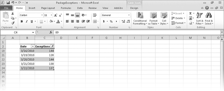
If you want to see the highest or lowest values in a data column, you can create a Top 10 filter. Choosing the Top 10 command from the menu doesn’t just limit the display to the top 10 values. Instead, it opens the Top 10 AutoFilter dialog box. From within this dialog box, you can choose whether to show values from the top or bottom of the list, define the number of items you want to see, and choose whether the number in the middle box indicates the number of items or the percentage of items to be shown when the filter is applied. Using the Top 10 AutoFilter dialog box, you can find your top 10 salespeople or identify the top 5 percent of your customers.
Excel 2010 includes a new capability called the search filter, which you can use to type a search string that Excel uses to identify which items to display in an Excel table or a data list. To use a search filter, click a column’s filter arrow and start typing a character string in the Search box. As you type the character string, Excel limits the items displayed at the bottom of the filter panel to those that contain the character or characters you’ve entered. When the filter list’s items represent the values you want to display, click OK.

When you point to Text Filters and then click Custom Filter, you can define a rule that Excel uses to decide which rows to show after the filter is applied. For instance, you can create a rule that determines that only days with package volumes of less than 100,000 should be shown in your worksheet. With those results in front of you, you might be able to determine whether the weather or another factor resulted in slower business on those days.
Excel indicates that a column has a filter applied by changing the appearance of the column’s filter arrow to include an icon that looks like a funnel. After you finish examining your data by using a filter, you can remove the filter by clicking the column’s filter arrow and then clicking Clear Filter. To turn off filtering entirely and remove the filter arrows, display the Home tab and then, in the Editing group, click Sort & Filter and then click Filter.
In this exercise, you’ll filter worksheet data by using a series of AutoFilter commands, create a filter showing the five days with the highest delivery exception counts in a month, create a search filter, and create a custom filter.
Note
SET UP You need the PackageExceptions_start workbook located in your Chapter12 practice file folder to complete this exercise. Start Excel, open the PackageExceptions_start workbook, and save it as PackageExceptions. Then follow the steps.
On the ByRoute worksheet, click any cell in the cell range B2:F27.
 On the Home tab, in
the Editing group, click Sort & Filter, and then click Filter.
On the Home tab, in
the Editing group, click Sort & Filter, and then click Filter.Click the Date column filter arrow and then, from the menu that appears, clear the March check box.
Excel changes the state of the Select All and 2010 check boxes to indicate that some items within those categories have been filtered.
Click OK.
Excel hides all rows that contain a date from the month of March.
Click the Center column filter arrow and then, from the menu that appears, clear the Select All check box.
Excel clears all the check boxes in the list.
On the Home tab, in the Editing group, click Sort & Filter, and then click Clear.
Excel clears all active filters but leaves the filter arrows in place.
Click the Route column header’s filter arrow, and then type RT9 in the Search box.
The filter list displays only routes with identifiers that include the characters RT9.
Click OK.
Excel applies the filter, displaying exceptions that occurred on routes with identifiers that contain the string RT9.
Click the MarchDailyCount sheet tab.
The MarchDailyCount worksheet appears.
Click any cell in the Excel table.
Click the Exceptions filter arrow, click Number Filters, and then click Top 10.
In the middle field, type 5.
Click OK.
Click the Exceptions column filter arrow, and then click Clear Filter from “Exceptions”.
Excel removes the filter.
Click the Date column filter arrow, click Date Filters, and then click Custom Filter.
In the upper-left list, click is after or equal to. In the upper-right list, click 3/8/2010. In the lower-left list, click is before or equal to. In the lower-right list, click 3/14/2010.
Click OK.
 On the Quick Access Toolbar, click the Undo button to remove your filter.


Excel offers a wide range of tools you can use to summarize worksheet data. This section shows you how to select rows at random using the RAND and RANDBETWEEN functions, how to summarize worksheet data using the SUBTOTAL and AGGREGATE functions, and how to display a list of unique values within a data set.
In addition to filtering the data that is stored in your Excel worksheets, you can choose rows at random from a list. Selecting rows randomly is useful for choosing which customers will receive a special offer, deciding which days of the month to audit, or picking prize winners at an employee party.
To choose rows randomly, you can use the RAND function, which generates a random value between 0 and 1, and compare the value it returns with a test value included in the formula. As an example, suppose Consolidated Messenger wanted to offer approximately 30 percent of its customers a discount on their next shipment. A formula that returns a TRUE value 30 percent of the time would be RAND<=0.3; that is, whenever the random value was between 0 and 0.3, the result would be TRUE. You could use this formula to select each row in a list with a probability of 30 percent. A formula that displayed TRUE when the value was equal to or less than 30 percent, and FALSE otherwise, would be =IF(RAND()<=0.3,“True”,“False”).
If you recalculate this formula 10 times, it’s very unlikely that you would see exactly three TRUE results and seven FALSE results. Just as flipping a coin can result in the same result 10 times in a row by chance, so can the RAND function’s results appear to be off if you only recalculate it a few times. However, if you were to recalculate the function 10 thousand times, it is extremely likely that the number of TRUE results would be very close to 30 percent.
Tip
Because the RAND function is a volatile function (it recalculates its results every time you update the worksheet), you should copy the cells that contain the RAND function in a formula and paste the formulas’ values back into their original cells. To do so, select the cells that contain the RAND formulas and press Ctrl+C to copy the cell’s contents. Then, on the Home tab, in the Clipboard group, in the Paste list, click Paste Values to replace the formula with its current result. If you don’t replace the formulas with their results, you will never have a permanent record of which rows were selected.
The RANDBETWEEN function generates a random whole number within a defined range. For example, the formula =RANDBETWEEN(1,100) would generate a random integer value from 1 to 100, inclusive. The RANDBETWEEN function is very useful for creating sample data collections for presentations. Before the RANDBETWEEN function was introduced, you had to create formulas that added, subtracted, multiplied, and divided the results of the RAND function, which are always decimal values between 0 and 1, to create your data.
Summarizing Worksheets with Hidden and Filtered Rows
The ability to analyze the data that’s most vital to your current needs is important, but there are some limitations to how you can summarize your filtered data by using functions such as SUM and AVERAGE. One limitation is that any formulas you create that include the SUM and AVERAGE functions don’t change their calculations if some of the rows used in the formula are hidden by the filter.
Excel provides two ways to summarize just the visible cells in a filtered data list. The first method is to use AutoCalculate. To use AutoCalculate, you select the cells you want to summarize. When you do, Excel displays the average of values in the cells, the sum of the values in the cells, and the number of visible cells (the count) in the selection.
To display the other functions you can use, right-click the status bar and select the function you want from the shortcut menu. If a check mark appears next to a function’s name, that function’s result appears on the status bar. Clicking a checked function name removes that function from the status bar.
AutoCalculate is great for finding a quick total or average for filtered cells, but it doesn’t make the result available in the worksheet. Formulas such as =SUM(C3:C26) always consider every cell in the range, regardless of whether you hide a cell’s row by right-clicking the row’s header and then clicking Hide, so you need to create a formula by using either the SUBTOTAL function or the AGGREGATE function (which is new in Excel 2010) to summarize just those values that are visible in your worksheet. The SUBTOTAL function enables you to summarize every value in a range or summarize only those values in rows you haven’t manually hidden. The SUBTOTAL function has this syntax: SUBTOTAL(function_num, ref1, ref2, …). The function_num argument holds the number of the operation you want to use to summarize your data. (The operation numbers are summarized in a table later in this section.) The ref1, ref2, and further arguments represent up to 29 ranges to include in the calculation.
As an example, assume you have a worksheet where you hid rows 20-26 manually. In this case, the formula =SUBTOTAL(9, C3:C26, E3:E26, G3:G26) would find the sum of all values in the ranges C3:C26, E3:E26, and G3:G26, regardless of whether that range contained any hidden rows. The formula =SUBTOTAL(109, C3:C26, E3:E26, G3:G26) would find the sum of all values in cells C3:C19, E3:E19, and G3:G19, ignoring the values in the manually hidden rows.
Important
Be sure to place your SUBTOTAL formula in a row that is even with or above the headers in the range you’re filtering. If you don’t, your filter might hide the formula’s result!
The following table lists the summary operations available for the SUBTOTAL formula. Excel displays the available summary operations as part of the Formula AutoComplete functionality, so you don’t need to remember the operation numbers or look them up in the Help system.
As the previous table shows, the SUBTOTAL function has two sets of operations. The first set (operations 1-11) represents operations that include hidden values in their summary, and the second set (operations 101-111) represents operations that summarize only values visible in the worksheet. Operations 1-11 summarize all cells in a range, regardless of whether the range contains any manually hidden rows. By contrast, the operations 101-111 ignore any values in manually hidden rows. What the SUBTOTAL function doesn’t do, however, is change its result to reflect rows hidden by using a filter.
The new AGGREGATE function extends the capabilities of the SUBTOTAL function. With it, you can select from a broader range of functions and use another argument to determine which, if any, values to ignore in the calculation. AGGREGATE has two possible syntaxes, depending on the summary operation you select. The first syntax is =AGGREGATE(function_num, options, ref1…), which is similar to the syntax of the SUBTOTAL function. The other possible syntax, =AGGREGATE(function_num, options, array, [k]), is used to create AGGREGATE functions that use the LARGE, SMALL, PERCENTILE.INC, QUARTILE.INC, PERCENTILE.EXC, and QUARTILE.EXC operations.
The following table summarizes the summary operations available for use in the AGGREGATE function.
|
Number |
Function |
Description |
|---|---|---|
|
1 |
AVERAGE |
Returns the average of the values in the range. |
|
2 |
COUNT |
Counts the cells in the range that contain a number. |
|
3 |
COUNTA |
Counts the nonblank cells in the range. |
|
4 |
MAX |
Returns the largest (maximum) value in the range. |
|
5 |
MIN |
Returns the smallest (minimum) value in the range. |
|
6 |
PRODUCT |
Returns the result of multiplying all numbers in the range. |
|
7 |
STDEV.S |
Calculates the standard deviation of values in the range by examining a sample of the values. |
|
8 |
STDEV.P |
Calculates the standard deviation of the values in the range by using all the values. |
|
9 |
SUM |
Returns the result of adding all numbers in the range together. |
|
10 |
VAR.S |
Calculates the variance of values in the range by examining a sample of the values. |
|
11 |
VAR.P |
Calculates the variance of the values in the range by using all of the values. |
|
12 |
MEDIAN |
Returns the value in the middle of a group of values. |
|
13 |
MODE.SNGL |
Returns the most frequently occurring number from a group of numbers. |
|
14 |
LARGE |
Returns the k-th largest value in a data set; k is specified using the last function argument. If k is left blank, Excel returns the largest value. |
|
15 |
SMALL |
Returns the k-th smallest value in a data set; k is specified using the last function argument. If k is left blank, Excel returns the smallest value. |
|
16 |
PERCENTILE.INC |
Returns the k-th percentile of values in a range, where k is a value from 0 to 1, inclusive. |
|
17 |
QUARTILE.INC |
Returns the quartile value of a data set, based on a percentage from 0 to 1, inclusive. |
|
18 |
PERCENTILE.EXC |
Returns the k-th percentile of values in a range, where k is a value from 0 to 1, exclusive. |
|
19 |
QUARTILE.EXC |
Returns the quartile value of a data set, based on a percentage from 0 to 1, exclusive. |
The second argument, options, enables you to select which items the AGGREGATE function should ignore. These items can include hidden rows, errors, and SUBTOTAL and AGGREGATE functions. The following table summarizes the values available for the options argument and the effect they have on the function’s results.
|
Number |
Description |
|---|---|
|
0 |
Ignore nested SUBTOTAL and AGGREGATE functions |
|
1 |
Ignore hidden rows and nested SUBTOTAL and AGGREGATE functions |
|
2 |
Ignore error values and nested SUBTOTAL and AGGREGATE functions |
|
3 |
Ignore hidden rows, error values, and nested SUBTOTAL and AGGREGATE functions |
|
4 |
Ignore nothing |
|
5 |
Ignore hidden rows |
|
6 |
Ignore error values |
|
7 |
Ignore hidden rows and error values |
Summarizing numerical values can provide valuable information that helps you run your business. It can also be helpful to know how many different values appear within a column. For example, you might want to display all of the countries in which Consolidated Messenger has customers. If you want to display a list of the unique values in a column, click any cell in the data set, display the Data tab and then, in the Sort & Filter group, click Advanced to display the Advanced Filter dialog box.

In the List Range field, type the reference of the cell range you want to examine for unique values, select the Unique Records Only check box, and then click OK to have Excel display the row that contains the first occurrence of each value in the column.
Important
Excel treats the first cell in the data range as a header cell, so it doesn’t consider the cell as it builds the list of unique values. Be sure to include the header cell in your data range!
In this exercise, you’ll select random rows from a list of exceptions to identify package delivery misadventures to investigate, create an AGGREGATE formula to summarize the visible cells in a filtered worksheet, and find the unique values in one column of data.
Note
SET UP You need the ForFollowUp_start workbook located in your Chapter12 practice file folder to complete this exercise. Open the ForFollowUp_start workbook, and save it as ForFollowUp. Then follow the steps.
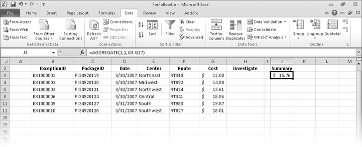
Select cells G3:G27.
The average of the values in the selected cells, the number of cells selected, and the total of the values in the selected cells appear in the AutoCalculate area of the status bar.
In cell J3, enter the formula =AGGREGATE(1,1,G3:G27).
The value $15.76 appears in cell J3.
 On the Data tab,
in the Sort & Filter group, click
Advanced.
On the Data tab,
in the Sort & Filter group, click
Advanced.In the List range field, type E2:E27.
Select the Unique records only check box, and then click OK.
Excel displays the rows that contain the first occurrence of each different value in the selected range.
Tip
Remember that you must include cell E2, the header cell, in the List Range field so that the filter doesn’t display two occurrences of Northeast in the unique values list. To see what happens when you don’t include the header cell, try changing the range in the List Range field to E3:E27, selecting the Unique Records Only check box, and then clicking OK.
 On the Data tab,
in the Sort & Filter group, click
Clear.
On the Data tab,
in the Sort & Filter group, click
Clear.Excel removes the filter.
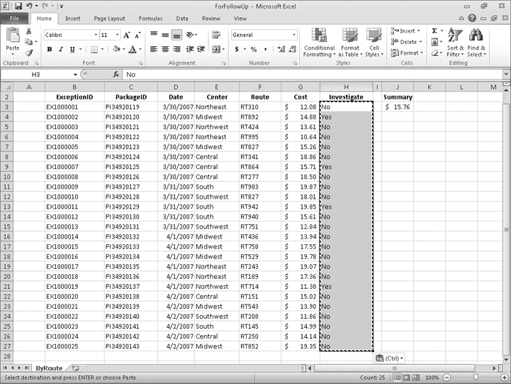
In cell H3, type the formula =IF(RAND()<0.15,“Yes”,“No”), and press Enter.
A value of Yes or No appears in cell H3, depending on the RAND function result.
Select cell H3, and then drag the fill handle down until it covers cell H27.
Excel copies the formula into every cell in the range H3:H27.
 With the range H3:H27 still selected, on the Home tab, in the Clipboard group, click the Copy button.
Excel copies the cell range’s contents to the Microsoft Office Clipboard.
 Click the Paste
arrow, and then in the Paste gallery
that appears, click the first icon in the Paste Values group.
Click the Paste
arrow, and then in the Paste gallery
that appears, click the first icon in the Paste Values group.Excel replaces the cells’ formulas with the formulas’ current results.
Part of creating efficient and easy-to-use worksheets is to do what you can to ensure the data entered into your worksheets is as accurate as possible. Although it isn’t possible to catch every typographical or transcription error, you can set up a validation rule to make sure that the data entered into a cell meets certain standards.
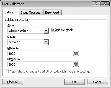
To create a validation rule, display the Data tab on the ribbon and then, in the Data Tools group, click the Data Validation button to open the Data Validation dialog box. You can use the controls in the Data Validation dialog box to define the type of data that Excel should allow in the cell and then, depending on the data type you choose, to set the conditions data must meet to be accepted in the cell. For example, you can set the conditions so that Excel knows to look for a whole number value between 1000 and 2000.
Setting accurate validation rules can help you and your colleagues avoid entering a customer’s name in the cell designated to hold the phone number or setting a credit limit above a certain level. To require a user to enter a numeric value in a cell, display the Settings page of the Data Validation dialog box, and, depending on your needs, choose either Whole Number or Decimal from the Allow list.
If you want to set the same validation rule for a group of cells, you can do so by selecting the cells to which you want to apply the rule (such as a column in which you enter the credit limit of customers of Consolidated Messenger) and setting the rule by using the Data Validation dialog box. One important fact you should keep in mind is that, with Excel, you can create validation rules for cells in which you have already entered data. Excel doesn’t tell you whether any of those cells contain data that violates your rule at the moment you create the rule, but you can find out by having Excel circle any worksheet cells containing data that violates the cell’s validation rule. To do so, display the Data tab and then, in the Data Tools group, click the Data Validation arrow. On the menu, click the Circle Invalid Data button to circle cells with invalid data.

Of course, it’s frustrating if you want to enter data into a cell and, when a message box appears that tells you the data you tried to enter isn’t acceptable, you aren’t given the rules you need to follow. With Excel, you can create a message that tells the user which values are expected before the data is entered and then, if the conditions aren’t met, reiterate the conditions in a custom error message.
You can turn off data validation in a cell by displaying the Settings page of the Data Validation dialog box and clicking the Clear All button in the lower-left corner of the dialog box.
In this exercise, you’ll create a data validation rule limiting the credit line of Consolidated Messenger customers to $25,000, add an input message mentioning the limitation, and then create an error message if someone enters a value greater than $25,000. After you create your rule and messages, you’ll test them.
Note
SET UP You need the Credit_start workbook located in your Chapter12 practice file folder to complete this exercise. Open the Credit_start workbook, and save it as Credit. Then follow the steps.
Select the cell range J4:J7.
Cell J7 is currently blank, but you will add a value to it later in this exercise.
 On the Data tab, in
the Data Tools group, click Data Validation.
On the Data tab, in
the Data Tools group, click Data Validation.The Data Validation dialog box opens and displays the Settings page.
In the Allow list, click Whole Number.
Boxes labeled Minimum and Maximum appear below the Data box.
In the Data list, click less than or equal to.
The Minimum box disappears.
In the Maximum box, type 25000.
Clear the Ignore blank check box.
The Input Message page is displayed.
In the Title box, type Enter Limit. In the Input Message box, type Please enter the customer’s credit limit, omitting the dollar sign and any commas.
Click the Error Alert tab. On the Error Alert page, in the Style list, click Stop.
The icon that appears on your message box changes to the Stop icon.
In the Title box, type Error, and then click OK.
Click cell J7.
A ScreenTip with the title Enter Limit and the text Please enter the customer’s credit limit, omitting the dollar sign and any commas appears near cell J7.
Type 25001, and press Enter.
A stop box with the title Error opens. Leaving the Error Message box blank in the Data Validation dialog box causes Excel to use its default message.
In the Error box, click Cancel.
Click cell J7.
Type 25000, and press Enter.
On the Data tab, in the Data Tools group, click the Data Validation arrow and then, in the list, click Circle Invalid Data.
A red circle appears around the value in cell J4.
In the Data Validation list, click Clear Validation Circles.
The red circle around the value in cell K4 disappears.


A number of filters are defined in Excel. (You might find the one you want is already available.)
Filtering an Excel worksheet based on values in a single column is easy to do, but you can create a custom filter to limit your data based on the values in more than one column as well.
With the new search filter capability in Excel 2010, you can limit the data in your worksheets based on characters the terms contain.
Don’t forget that you can get a running total (or an average, or any one of several other summary operations) for the values in a group of cells. Just select the cells and look on the status bar: the result will be there.
Use data validation techniques to improve the accuracy of data entered into your worksheets and to identify data that doesn’t meet the guidelines you set.