
Chapter at a Glance

Entering data into a workbook efficiently saves you time, but you must also ensure that your data is easy to read. Microsoft Excel 2010 gives you a wide variety of ways to make your data easier to understand; for example, you can change the font, character size, or color used to present a cell’s contents. Changing how data appears on a worksheet helps set the contents of a cell apart from the contents of surrounding cells. The simplest example of that concept is a data label. If a column on your worksheet contains a list of days, you can easily set apart a label (for example, Day) by presenting it in bold type that’s noticeably larger than the type used to present the data to which it refers. To save time, you can define a number of custom formats and then apply them quickly to the desired cells.
You might also want to specially format a cell’s contents to reflect the value in that cell. For example, Lori Penor, the chief operating officer of Consolidated Messenger, might want to create a worksheet that displays the percentage of improperly delivered packages from each regional distribution center. If that percentage exceeds a threshold, she could have Excel display a red traffic light icon, indicating that the center’s performance is out of tolerance and requires attention.
In this chapter, you’ll learn how to change the appearance of data, apply existing formats to data, make numbers easier to read, change data’s appearance based on its value, and add images to worksheets.
Note
Practice Files Before you can complete the exercises in this chapter, you need to copy the book’s practice files to your computer. The practice files you’ll use to complete the exercises in this chapter are in the Chapter11 practice file folder. A complete list of practice files is provided in Using the Practice Files at the beginning of this book.
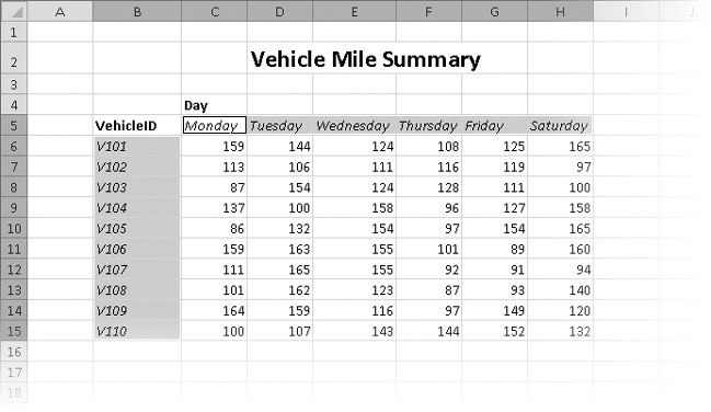
Excel spreadsheets can hold and process lots of data, but when you manage numerous spreadsheets it can be hard to remember from a worksheet’s title exactly what data is kept in that worksheet. Data labels give you and your colleagues information about data in a worksheet, but it’s important to format the labels so that they stand out visually. To make your data labels or any other data stand out, you can change the format of the cells that hold your data.
Most of the tools you need to change a cell’s format can be found on the Home tab. You can apply the formatting represented on a button by selecting the cells you want to apply the style to and then clicking that button. If you want to set your data labels apart by making them appear bold, click the Bold button. If you have already made a cell’s contents bold, selecting the cell and clicking the Bold button will remove the formatting.
Tip
Deleting a cell’s contents doesn’t delete the cell’s formatting. To delete a selected cell’s formatting, on the Home tab, in the Editing group, click the Clear button (which looks like an eraser), and then click Clear Formats. Clicking Clear All from the same list will remove the cell’s contents and formatting.
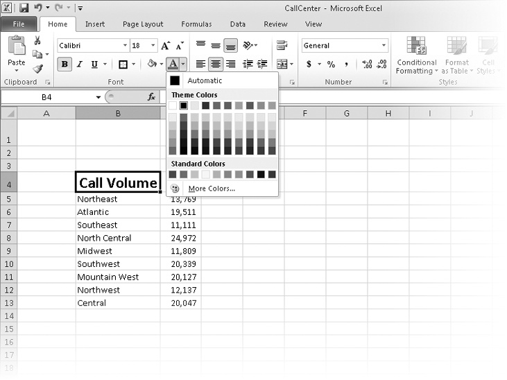
Buttons in the Home tab’s Font group that give you choices, such as the Font Color button, have an arrow at the right edge of the button. Clicking the arrow displays a list of options accessible for that button, such as the fonts available on your system or the colors you can assign to a cell.
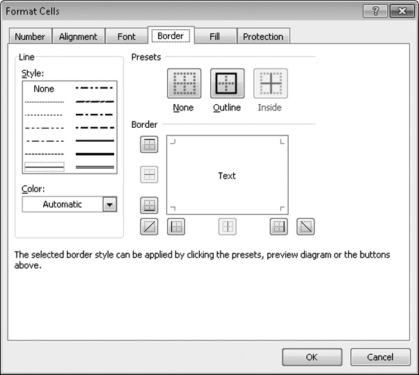
Another way you can make a cell stand apart from its neighbors is to add a border around the cell. To place a border around one or more cells, select the cells, and then choose the border type you want by selecting from the Border list in the Font group. Excel does provide more options: To display the full range of border types and styles, in the Border list, click More Borders. The Format Cells dialog box opens, displaying the Border page.
You can also make a group of cells stand apart from its neighbors by changing its shading, which is the color that fills the cells. On a worksheet that tracks total package volume for the past month, Lori Penor could change the fill color of the cells holding her data labels to make the labels stand out even more than by changing the labels’ text formatting.
Tip
You can display the most commonly used formatting controls by right-clicking a selected range. When you do, a Mini Toolbar containing a subset of the Home tab formatting tools appears above the shortcut menu.
If you want to change the attributes of every cell in a row or column, you can click the header of the row or column you want to modify and then select your desired format.
One task you can’t perform by using the tools on the Home tab is to change the standard font for a workbook, which is used in the Name box and on the formula bar. The standard font when you install Excel is Calibri, a simple font that is easy to read on a computer screen and on the printed page. If you want to choose another font, click the File tab, and then click Options. On the General page of the Excel Options dialog box, set the values in the Use This Font and Font Size list boxes to pick your new display font.
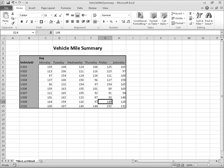
In this exercise, you’ll emphasize a worksheet’s title by changing the format of cell data, adding a border to a cell range, and then changing a cell range’s fill color. After those tasks are complete, you’ll change the default font for the workbook.
Note
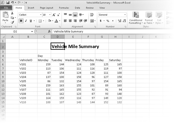
SET UP You need the VehicleMileSummary_start workbook located in your Chapter11 practice file folder to complete this exercise. Start Excel, open the VehicleMileSummary_start workbook, and save it as VehicleMileSummary. Then follow the steps.
Click cell D2.
 In the Font group,
click the Font Size arrow, and then in
the list, click 18.
In the Font group,
click the Font Size arrow, and then in
the list, click 18.Click cell B5, hold down the Ctrl key, and click cell C4 to select the non-contiguous cells.
On the Home tab, in the Font group, click the Bold button.
Excel displays the cells’ contents in bold type.
Select the cell ranges B6:B15 and C5:H5.
 In the Font group,
click the Border arrow, and then in the
list, click Outside Borders.
In the Font group,
click the Border arrow, and then in the
list, click Outside Borders.Excel places a border around the outside edge of the selected cells.
Select the cell range B4:H15.
In the Border list, click Thick Box Border.
Excel places a thick border around the outside edge of the selected cells.
Select the cell ranges B4:B15 and C4:H5.
 In the Font group,
click the Fill Color arrow, and then in
the Standard Colors area of the color
palette, click the yellow button.
In the Font group,
click the Fill Color arrow, and then in
the Standard Colors area of the color
palette, click the yellow button.Excel changes the selected cells’ background color to yellow.
Note
Troubleshooting The appearance of buttons and groups on the ribbon changes depending on the width of the program window. For information about changing the appearance of the ribbon to match our screen images, see Modifying the Display of the Ribbon at the beginning of this book.
Click the File tab, and then click Options.
If necessary, click General to display the General page.
In the When creating new workbooks area, in the Use this font list, click Verdana.
Verdana appears in the Use This Font field.
Click Cancel.
The Excel Options dialog box closes without saving your change.
As you work with Excel, you will probably develop preferred formats for data labels, titles, and other worksheet elements. Instead of adding a format’s characteristics one element at a time to the target cells, you can have Excel store the format and recall it as needed. You can find the predefined formats by displaying the Home tab, and then in the Styles group, clicking Cell Styles.
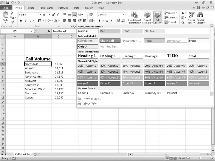
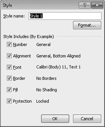
Clicking a style from the Cell Styles gallery applies the style to the selected cells, but Excel also displays a live preview of a format when you point to it. If none of the existing styles is what you want, you can create your own style by clicking New Cell Style at the bottom of the gallery to display the Style dialog box. In the Style dialog box, type the name of your new style in the Style Name field, and then click Format. The Format Cells dialog box opens.
After you set the characteristics of your new style, click OK to make your style available in the Cell Styles gallery. If you ever want to delete a custom style, display the Cell Styles gallery, right-click the style, and then click Delete.
If all you want to do is apply formatting from one cell to the contents of another cell, use the Format Painter tool in the Clipboard group on the Home tab. Just click the cell that has the format you want to copy, click the Format Painter button, and then click the cells to which you want to apply the copied format. To apply the same formatting to multiple cells, double-click the Format Painter button and then click the target cells. When you’re done applying the formatting, press the Esc key.
In this exercise, you’ll create a style and apply the new style to a data label.
Note
SET UP You need the HourlyExceptions_start workbook located in your Chapter11 practice file folder to complete this exercise. Open the HourlyExceptions_start workbook, and save it as HourlyExceptions. Then follow the steps.
 On the Home tab, in
the Styles group, click Cell Styles, and then click New Cell Style.
On the Home tab, in
the Styles group, click Cell Styles, and then click New Cell Style.In the Style name field, type Crosstab Column Heading.
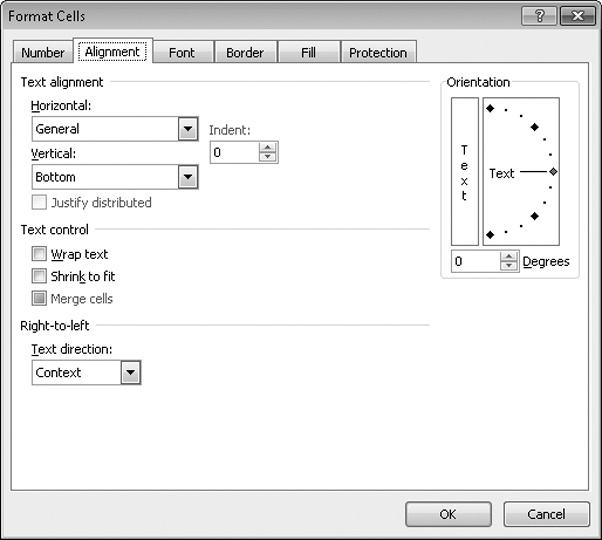
Click the Format button. In the Format Cells dialog box, click the Alignment tab.
In the Horizontal list, click Center.
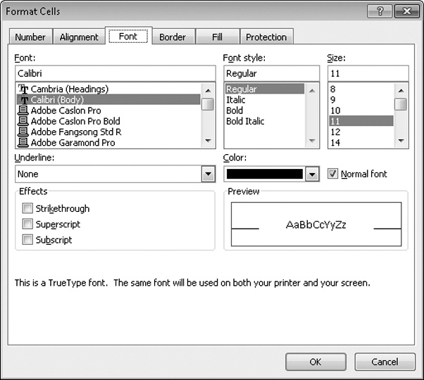
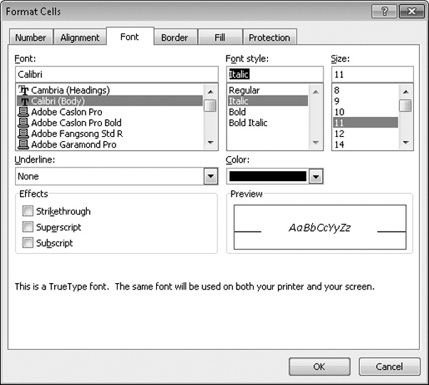
Click the Font tab.
In the Font style list, click Italic.
The text in the Preview pane appears in italicized text.
The Number page of the Format Cells dialog box is displayed.
In the Category list, click Time.
The available time formats appear.
In the Type pane, click 1:30 PM.
Click OK to save your changes.
The Format Cells dialog box closes, and your new style’s definition appears in the Style dialog box.
Click OK.
The Style dialog box closes.
Select cells C4:N4.
On the Home tab, in the Styles group, click Cell Styles.
The Cell Styles gallery opens.
Click the Crosstab Column Heading style.
Excel applies your new style to the selected cells.

Microsoft Office 2010 includes powerful design tools that enable you to create attractive, professional documents quickly. The Excel product team implemented the new design capabilities by defining workbook themes and Excel table styles. A theme is a way to specify the fonts, colors, and graphic effects that appear in a workbook. Excel comes with many themes installed.
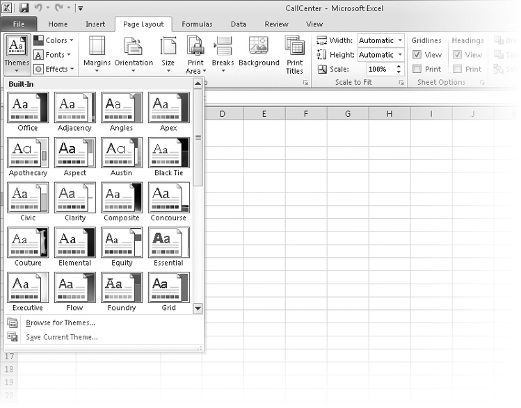
To apply an existing workbook theme, display the Page Layout tab. Then, in the Themes group, click Themes, and click the theme you want to apply to your workbook. By default, Excel applies the Office theme to your workbooks.
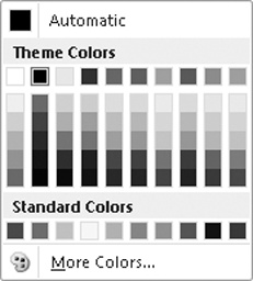
When you want to format a workbook element, Excel displays colors that are available within the active theme. For example, selecting a worksheet cell and then clicking the Font Color arrow displays a palette of colors. The theme colors appear at the top of the color palette—the standard colors and the More Colors link, which displays the Colors dialog box, appear at the bottom of the palette.
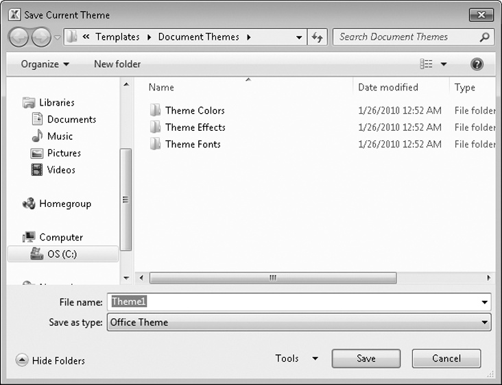
You can change a theme’s colors, fonts, and graphic effects by displaying the Page Layout tab and then, in the Themes group, selecting new values from the Colors, Fonts, and Effects lists. To save your changes as a new theme, display the Page Layout tab, and in the Themes group, click Themes, and then click Save Current Theme. Use the controls in the Save Current Theme dialog box that opens to record your theme for later use. Later, when you click the Themes button, your custom theme will appear at the top of the gallery.
Tip
When you save a theme, you save it as an Office Theme file. You can apply the theme to other Office 2010 documents as well.
Just as you can define and apply themes to entire workbooks, you can apply and define Excel table styles. You select an Excel table’s initial style when you create it; to create a new style, display the Home tab, and in the Styles group, click Format As Table. In the Format As Table gallery, click New Table Style to display the New Table Quick Style dialog box.

Type a name for the new style, select the first table element you want to format, and then click Format to display the Format Cells dialog box. Define the element’s formatting, and then click OK. When the New Table Quick Style dialog box reopens, its Preview pane displays the overall table style and the Element Formatting area describes the selected element’s appearance. Also, in the Table Element list, Excel displays the element’s name in bold to indicate it has been changed. To make the new style the default for new Excel tables created in the current workbook, select the Set As Default Table Quick Style For This Document check box. When you click OK, Excel saves the new table style.
Tip
To remove formatting from a table element, click the name of the table element and then click the Clear button.
In this exercise, you’ll create a new workbook theme, change a workbook’s theme, create a new table style, and apply the new style to an Excel table.
Note
SET UP You need the HourlyTracking_start workbook located in your Chapter11 practice file folder to complete this exercise. Open the HourlyTracking_start workbook, and save it as HourlyTracking. Then follow the steps.
If necessary, click any cell in the Excel table.
 On the Home tab, in
the Styles group, click Format as Table, and then click the style at
the upper-left corner of the Table
Styles gallery.
On the Home tab, in
the Styles group, click Format as Table, and then click the style at
the upper-left corner of the Table
Styles gallery.Excel applies the style to the table.
On the Home tab, in the Styles group, click Format as Table, and then click New Table Style.
The New Table Quick Style dialog box opens.
In the Name field, type Exception Default.
In the Table Element list, click Header Row.
Click Format.
The Format Cells dialog box opens.
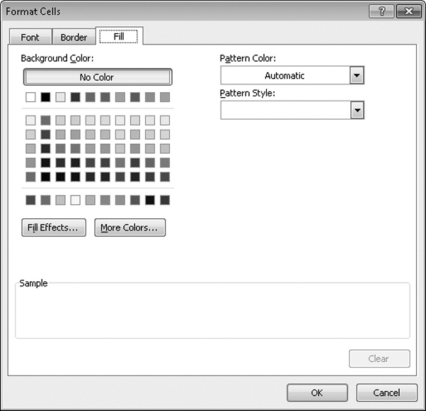
Click the Fill tab.
In the first row of color squares, just below the No Color button, click the third square from the left.
The new background color appears in the Sample pane of the dialog box.
Click OK.
The Format Cells dialog box closes. When the New Table Quick Style dialog box reopens, the Header Row table element appears in bold, and the Preview pane’s header row is shaded.
In the Table Element list, click Second Row Stripe, and then click Format.
The Format Cells dialog box opens.
Just below the No Color button, click the third square from the left again.
The new background color appears in the Sample pane of the dialog box.
Click OK.
The Format Cells dialog box closes. When the New Table Quick Style dialog box reopens, the Second Row Stripe table element appears in bold, and every second row is shaded in the Preview pane.
Click OK.
The New Table Quick Style dialog box closes.
On the Home tab, in the Styles group, click Format as Table. In the gallery, in the Custom area, click the new format.
Excel applies the new format.
 On the Page Layout
tab, in the Themes group, click the
Fonts arrow, and then in the list,
click Verdana.
On the Page Layout
tab, in the Themes group, click the
Fonts arrow, and then in the list,
click Verdana.Excel changes the theme’s font to Verdana (which is part of the Aspect font set).
 In the Themes group,
click the Themes button, and then click
Save Current Theme.
In the Themes group,
click the Themes button, and then click
Save Current Theme.In the File name field, type Verdana Office, and then click Save.
Excel saves your theme.
In the Themes group, click the Themes button, and then click Origin.
Excel applies the new theme to your workbook.


Changing the format of the cells in your worksheet can make your data much easier to read, both by setting data labels apart from the actual data and by adding borders to define the boundaries between labels and data even more clearly. Of course, using formatting options to change the font and appearance of a cell’s contents doesn’t help with idiosyncratic data types such as dates, phone numbers, or currency values.
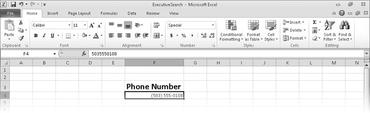
As an example, consider U.S. phone numbers. These numbers are 10 digits long and have a 3-digit area code, a 3-digit exchange, and a 4-digit line number written in the form (###) ###-####. Although it’s certainly possible to type a phone number with the expected formatting in a cell, it’s much simpler to type a sequence of 10 digits and have Excel change the data’s appearance.
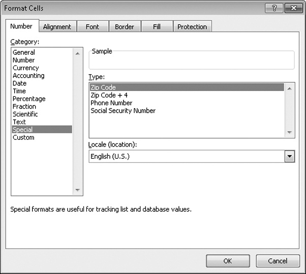
You can tell Excel to expect a phone number in a cell by opening the Format Cells dialog box to the Number page and displaying the formats available for the Special category.
Clicking Phone Number in the Type list tells Excel to format 10-digit numbers in the standard phone number format. You can see this in operation if you compare the contents of the active cell and the contents of the formula box for a cell with the Phone Number formatting.
Note
Troubleshooting If you type a 9-digit number in a field that expects a phone number, you won’t see an error message; instead, you’ll see a 2-digit area code. For example, the number 425550012 would be displayed as (42) 555-0012. An 11-digit number would be displayed with a 4-digit area code. If the phone number doesn’t look right, you probably left out a digit or included an extra one, so you should make sure your entry is correct.
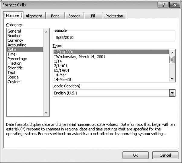
Just as you can instruct Excel to expect a phone number in a cell, you can also have it expect a date or a currency amount. You can make those changes from the Format Cells dialog box by choosing either the Date category or the Currency category. The Date category enables you to pick the format for the date (and determine whether the date’s appearance changes due to the Locale setting of the operating system on the computer viewing the workbook). In a similar vein, selecting the Currency category displays controls to set the number of places after the decimal point, the currency symbol to use, and the way in which Excel should display negative numbers.
Tip
The Excel user interface enables you to make the most common format changes by displaying the Home tab of the ribbon and then, in the Number group, either clicking a button representing a built-in format or selecting a format from the Number Format list.
You can also create a custom numeric format to add a word or phrase to a number in a cell. For example, you can add the phrase per month to a cell with a formula that calculates average monthly sales for a year to ensure that you and your colleagues will recognize the figure as a monthly average. To create a custom number format, click the Home tab, and then click the Number dialog box launcher (found at the bottom right corner of the Number group on the ribbon) to display the Format Cells dialog box. Then, if necessary, click the Number tab.
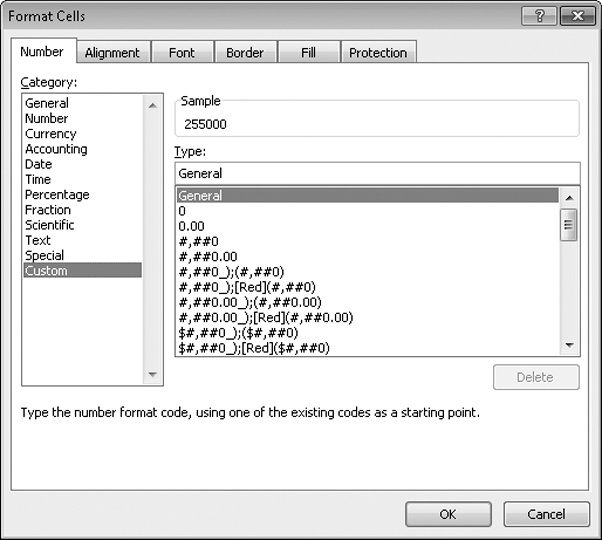
In the Category list, click Custom to display the available custom number formats in the Type list. You can then click the base format you want and modify it in the Type box. For example, clicking the 0.00 format causes Excel to format any number in a cell with two digits to the right of the decimal point.
Tip
The zeros in the format indicate that the position in the format can accept any number as a valid value.
To customize the format, click in the Type box and add any symbols or text you want to the format. For example, typing a dollar ($) sign to the left of the existing format and then typing “per month” (including quote marks) to the right of the existing format causes the number 1500 to be displayed as $1500.00 per month.
Important
You need to enclose any text to be displayed as part of the format in quotes so that Excel recognizes the text as a string to be displayed in the cell.
In this exercise, you’ll assign date, phone number, and currency formats to ranges of cells.
Note
SET UP You need the ExecutiveSearch_start workbook located in your Chapter11 practice file folder to complete this exercise. Open the ExecutiveSearch_start workbook, and save it as ExecutiveSearch. Then follow the steps.
Click cell A3.
On the Home tab, click the Font dialog box launcher.
The Format Cells dialog box opens.
If necessary, click the Number tab.
In the Category list, click Date.
The Type list appears with a list of date formats.
In the Type list, click 3/14/01.
Click OK to assign the chosen format to the cell.
Excel displays the contents of cell A3 to reflect the new format.
 On the Home tab, in
the Number group, click the Number Format button’s down arrow and
then click More Number Formats.
On the Home tab, in
the Number group, click the Number Format button’s down arrow and
then click More Number Formats.If necessary, click the Number tab in the Format Cells dialog box.
In the Category list, click Special.
The Type list appears with a list of special formats.
In the Type list, click Phone Number, and then click OK.
Excel displays the contents of the cell as (425) 555-0102, matching the format you selected, and the Format Cells dialog box closes.
Click cell H3.
Click the Font dialog box launcher.
In the Format Cells dialog box that opens, click the Number tab.
In the Category list, click Custom.
The contents of the Type list are updated to reflect your choice.
In the Type list, click the #,##0 item.
In the Type box, click to the left of the existing format, and type $. Then click to the right of the format, and type “before bonuses” (note the space after the opening quote).
Click OK.
The Format Cells dialog box closes.

Recording package volumes, vehicle miles, and other business data in a worksheet enables you to make important decisions about your operations. And as you saw earlier in this chapter, you can change the appearance of data labels and the worksheet itself to make interpreting your data easier.
Another way you can make your data easier to interpret is to have Excel change the appearance of your data based on its value. These formats are called conditional formats because the data must meet certain conditions, defined in conditional formatting rules, to have a format applied to it. For example, if chief operating officer Lori Penor wanted to highlight any Thursdays with higher-than-average weekday package volumes, she could define a conditional format that tests the value in the cell recording total sales and changes the format of the cell’s contents when the condition is met.
To create a conditional format, you select the cells to which you want to apply the format, display the Home tab, and then in the Styles group, click Conditional Formatting to display a menu of possible conditional formats. In Excel, you can define conditional formats that change how the program displays data in cells that contain values above or below the average values of the related cells, that contain values near the top or bottom of the value range, or that contain values duplicated elsewhere in the selected range.
When you select which kind of condition to create, Excel displays a dialog box that contains fields and controls you can use to define your rule. To display all of the rules for the selected cells, display the Home tab, and then in the Styles group, click Conditional Formatting. On the menu, click Manage Rules to display the Conditional Formatting Rules Manager.
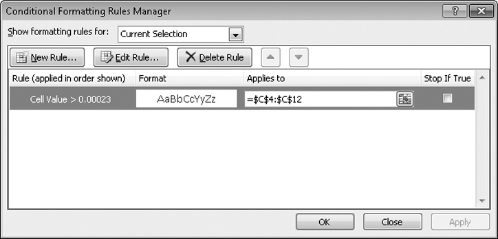
The Conditional Formatting Rules Manager enables you to control your conditional formats in the following ways:
Create a new rule by clicking the New Rule button.
Change a rule by clicking the rule and then clicking the Edit Rule button.
Remove a rule by clicking the rule and then clicking the Delete Rule button.
Move a rule up or down in the order by clicking the rule and then clicking the Move Up button or Move Down button.
Control whether Excel continues evaluating conditional formats after it finds a rule to apply by selecting or clearing a rule’s Stop If True check box.
Save any new rules and close the Conditional Formatting Rules Manager by clicking OK.
Save any new rules without closing the Conditional Formatting Rules Manager by clicking Apply.
Discard any unsaved changes by clicking Cancel.
Tip
Clicking the New Rule button in the Conditional Formatting Rules Manager opens the New Formatting Rule dialog box. The commands in the New Formatting Rule dialog box duplicate the options displayed when you click the Conditional Formatting button in the Styles group on the Home tab.
After you create a rule, you can change the format applied if the rule is true by clicking the rule and then clicking the Edit Rule button to display the Edit Formatting Rule dialog box. In that dialog box, click the Format button to display the Format Cells dialog box. After you define your format, click OK to display the rule.

Important
Excel doesn’t check to make sure that your conditions are logically consistent, so you need to be sure that you plan and enter your conditions correctly.
Excel also enables you to create three other types of conditional formats: data bars, color scales, and icon sets.
When data bars were introduced in Excel 2007, they filled cells with a color band that decreased in intensity as it moved across the cell. This gradient fill pattern made it a bit difficult to determine the relative length of two data bars because the end points weren’t as distinct as they would have been if the bars were a solid color. Excel 2010 enables you to choose between a solid fill pattern, which makes the right edge of the bars easier to discern, and a gradient fill, which you can use if you share your workbook with colleagues who use Excel 2007.
Excel also draws data bars differently than was done in Excel 2007. Excel 2007 drew a very short data bar for the lowest value in a range and a very long data bar for the highest value. The problem was that similar values could be represented by data bars of very different lengths if there wasn’t much variance among the values in the conditionally formatted range. In Excel 2010, data bars compare values based on their distance from zero, so similar values are summarized using data bars of similar lengths.
Tip
Excel 2010 data bars summarize negative values by using bars that extend to the left of a baseline that the program draws in a cell. You can control how your data bars summarize negative values by clicking the Negative Value And Axis button, which can be accessed from either the New Formatting Rule dialog box or the Edit Formatting Rule dialog box.
Color scales compare the relative magnitude of values in a cell range by applying colors from a two-color or three-color set to your cells.

Icon sets are collections of images that Excel displays when certain rules are met.
When icon sets were introduced in Excel 2007, you could apply an icon set as a whole, but you couldn’t create custom icon sets or choose to have Excel 2007 display no icon if the value in a cell met a criterion. In Excel 2010, you can display any icon from any set for any criterion or display no icon.
When you click a color scale or icon set in the Conditional Formatting Rules Manager and then click the Edit Rule button, you can control when Excel applies a color or icon to your data.
Important
Be sure to not include cells that contain summary formulas in your conditionally formatted ranges. The values, which could be much higher or lower than your regular cell data, could throw off your comparisons.
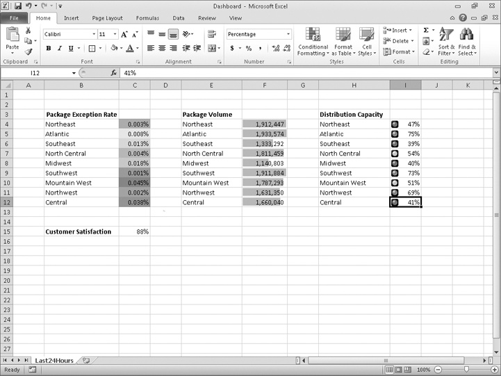
In this exercise, you’ll create a series of conditional formats to change the appearance of data in worksheet cells displaying the package volume and delivery exception rates of a regional distribution center.
Note
SET UP You need the Dashboard_start workbook located in your Chapter11 practice file folder to complete this exercise. Open the Dashboard_start workbook, and save it as Dashboard. Then follow the steps.
 On the Home tab, in
the Styles group, click Conditional Formatting. On the menu, point to Color Scales, and then in the
top row of the palette, click the second pattern from the left.
On the Home tab, in
the Styles group, click Conditional Formatting. On the menu, point to Color Scales, and then in the
top row of the palette, click the second pattern from the left.Select cells F4:F12.
On the Home tab, in the Styles group, click Conditional Formatting. On the menu, point to Data Bars, and then, in the Solid Fill group, click the orange data bar format.
Excel formats the selected range.
Select cells I4:I12.
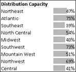
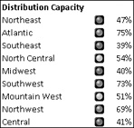
On the Home tab, in the Styles group, click Conditional Formatting. On the menu, point to Icon Sets, and then in the left column of the list of formats, click the three traffic lights with black borders.
With the range I4:I12 still selected, on the Home tab, in the Styles group, click Conditional Formatting, and then click Manage Rules.
Click the Reverse Icon Order button.
Excel reconfigures the rules so the red light icon is at the top and the green light icon is at the bottom.
In the red light icon’s row, in the Type list, click Number.
In the red light icon’s Value field, type 0.7.
In the yellow light icon’s row, in the Type list, click Number.
In the yellow light icon Value field, type 0.5.
Click OK twice to close the Edit Formatting Rule dialog box and the Conditional Formatting Rules Manager.
Excel formats the selected cell range.
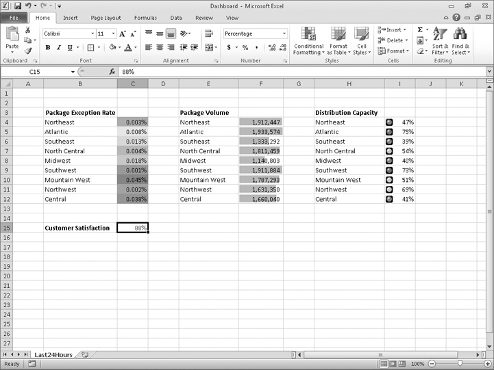
Click cell C15.
On the Home tab, in the Styles group, click Conditional Formatting. On the menu, point to Highlight Cells Rules, and then click Less Than.
The Less Than dialog box opens.
In the left field, type 96%.
Click OK.
The Less Than dialog box closes, and Excel displays the text in cell C15 in red.


Establishing a strong corporate identity helps customers remember your organization as well as the products and services you offer. Setting aside the obvious need for sound management, two important physical attributes of a strong retail business are a well-conceived shop space and an eye-catching, easy-to-remember logo. After you or your graphic artist has created a logo, you should add the logo to all your documents, especially any that might be seen by your customers. Not only does the logo mark the documents as coming from your company but it also serves as an advertisement, encouraging anyone who sees your worksheets to call or visit your company.
One way to add a picture to a worksheet is to display the Insert tab, and then in the Illustrations group, click Picture. Clicking Picture displays the Insert Picture dialog box, from which you can locate the picture you want to add from your hard disk. When you insert a picture, the Picture Tools Format contextual tab appears on the ribbon. You can use the tools on the Format contextual tab to change the picture’s contrast, brightness, and other attributes. With the controls in the Picture Styles group, you can place a border around the picture, change the picture’s shape, or change a picture’s effects (such as shadow, reflection, or three-dimensional effects). Other tools, found in the Arrange and Size groups, enable you to rotate, reposition, and resize the picture.
You can also resize a picture by clicking it and then dragging one of the handles that appears on the graphic. If you accidentally resize a graphic by dragging a handle, just click the Undo button to remove your change.
Excel 2010 includes a new built-in capability that you can use to remove the background of an image you insert into a workbook. To do so, click the image and then, on the Format contextual tab of the ribbon, in the Adjust group, click Remove Background. When you do, Excel attempts to identify the foreground and background of the image.

You can drag the handles on the inner square of the background removal tool to change how the tool analyzes the image. When you have adjusted the outline to identify the elements of the image you want to keep, click the Keep Changes button on the Background Removal contextual tab of the ribbon to complete the operation.
If you want to generate a repeating image in the background of a worksheet to form a tiled pattern behind your worksheet’s data, you can display the Page Layout tab, and then in the Page Setup group, click Background. In the Sheet Background dialog box, click the image that you want to serve as the background pattern for your worksheet, and click OK.
Tip
To remove a background image from a worksheet, display the Page Layout tab, and then in the Page Setup group, click Delete Background.
To achieve a watermark-type effect with words displayed behind the worksheet data, save the watermark information as an image, and then use the image as the sheet background; you could also insert the image in the header or footer, and then resize or scale it to position the watermark information where you want it.
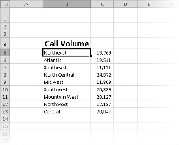
In this exercise, you’ll add an image to an existing worksheet, change its location on the worksheet, reduce the size of the image, and then set another image as a repeating background for the worksheet.
Note
SET UP You need the CallCenter_start workbook and the Phone and Texture images located in your Chapter11 practice file folder to complete this exercise. Open the CallCenter_start workbook, and save it as CallCenter. Then follow the steps.
 On the Insert tab,
in the Illustrations group, click Picture.
On the Insert tab,
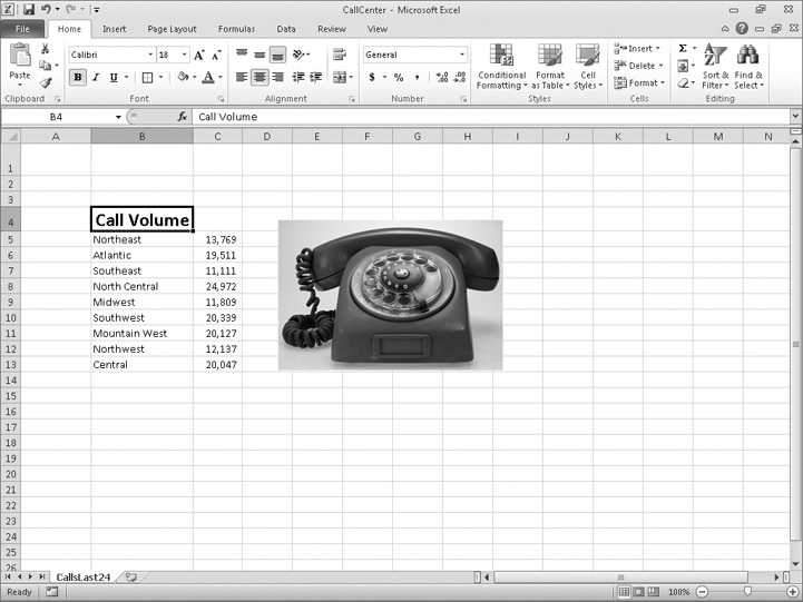
in the Illustrations group, click Picture.Navigate to the Chapter11 practice file folder, and then double-click the Phone image file.
The image appears on your worksheet.
 On the Format
contextual tab, in the Adjust group,
click Remove Background.
On the Format
contextual tab, in the Adjust group,
click Remove Background.Excel attempts to separate the image’s foreground from its background.
Drag the handles at the upper-left and bottom-right corners of the outline until the entire phone, including the cord, is within the frame.
On the Background Removal tab, click Keep Changes.
Excel removes the highlighted image elements.
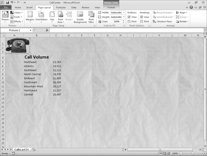
Move the image to the upper-left corner of the worksheet, click and hold the handle at the lower-right corner of the image, and drag it up and to the left until the image no longer obscures the Call Volume label.
 On the Page Layout
tab, in the Page Setup group, click
Background.
On the Page Layout
tab, in the Page Setup group, click
Background.Navigate to the Chapter11 practice file folder, and then double-click the Texture image file.
 On the Page Layout
tab, in the Page Setup group, click
Delete Background.
On the Page Layout
tab, in the Page Setup group, click
Delete Background.


If you don’t like the default font in which Excel displays your data, you can change it.
You can use cell formatting, including borders, alignment, and fill colors, to emphasize certain cells in your worksheets. This emphasis is particularly useful for making column and row labels stand out from the data.
Excel comes with a number of existing styles that enable you to change the appearance of individual cells. You can also create new styles to make formatting your workbooks easier.
If you want to apply the formatting from one cell to another cell, use the Format Painter to copy the format quickly.
There are quite a few built-in document themes and Excel table formats you can apply to groups of cells. If you see one you like, use it and save yourself lots of formatting time.
Conditional formats enable you to set rules so that Excel changes the appearance of a cell’s contents based on its value.
Adding images can make your worksheets more visually appealing and make your data easier to understand. Excel 2010 greatly enhances your ability to manage your images without leaving Excel.