
Chapter at a Glance
Microsoft Excel 2010 workbooks give you a handy place to store and organize your data, but you can also do a lot more with your data in Excel. One important task you can perform is to calculate totals for the values in a series of related cells. You can also use Excel to discover other information about the data you select, such as the maximum or minimum value in a group of cells. By finding the maximum or minimum value in a group, you can identify your best salesperson, product categories you might need to pay more attention to, or suppliers that consistently give you the best deal. Regardless of your bookkeeping needs, Excel gives you the ability to find the information you want. And if you make an error, you can find the cause and correct it quickly.
Many times, you can’t access the information you want without referencing more than one cell, and it’s also often true that you’ll use the data in the same group of cells for more than one calculation. Excel makes it easy to reference a number of cells at once, enabling you to define your calculations quickly.
In this chapter, you’ll learn how to streamline references to groups of data on your worksheets and how to create and correct formulas
Note
Practice Files Before you can complete the exercises in this chapter, you need to copy the book’s practice files to your computer. The practice files you’ll use to complete the exercises in this chapter are in the Chapter10 practice file folder. A complete list of practice files is provided in Using the Practice Files at the beginning of this book.
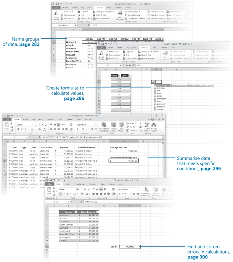
When you work with large amounts of data, it’s often useful to identify groups of cells that contain related data. For example, you can create a worksheet in which cells C4:I4 hold the number of packages Consolidated Messenger’s Northeast processing facility handled from 5:00 P.M. to 12:00 A.M. on the previous day.

Instead of specifying the cells individually every time you want to use the data they contain, you can define those cells as a range (also called a named range). For example, you can group the items from the cells described in the preceding paragraph into a range named NortheastPreviousDay. Whenever you want to use the contents of that range in a calculation, you can simply use the name of the range instead of specifying each cell individually.
Tip
Yes, you could just name the range Northeast, but if you use the range’s values in a formula in another worksheet, the more descriptive range name tells you and your colleagues exactly what data is used in the calculation.
To create a named range, select the cells you want to include in your range, click the Formulas tab, and then, in the Defined Names group, click Define Name to display the New Name dialog box. In the New Name dialog box, type a name in the Name field, verify that the cells you selected appear in the Refers To field, and then click OK. You can also add a comment about the range in the Comment field and select whether you want to make the name available for formulas in the entire workbook or just on an individual worksheet.
If the cells you want to define as a named range have labels in a row or column that’s part of the cell group, you can use those labels as the names of the named ranges. For example, if your data appears in worksheet cells B4:I12 and the values in column B are the row labels, you can make each row its own named range. To create a series of named ranges from a group of cells, select all of the data cells, including the labels, display the Formulas tab and then, in the Defined Names group, click Create From Selection to display the Create Names From Selection dialog box. In the Create Names From Selection dialog box, select the check box that represents the labels’ position in the selected range, and then click OK.

A final way to create a named range is to select the cells you want in the range, click in the Name box next to the formula box, and then type the name for the range.

To manage the named ranges in a workbook, display the Formulas tab, and then, in the Defined Names group, click Name Manager to display the Name Manager dialog box.
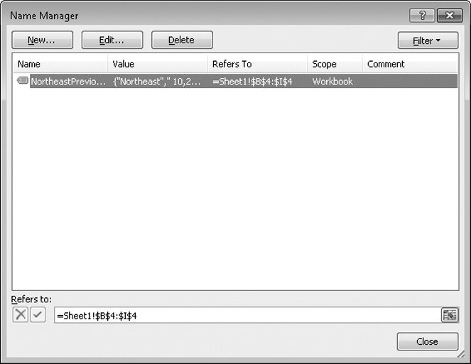
Clicking the Edit button displays the Edit Name dialog box, which is a version of the New Name dialog box, enabling you to change a named range’s definition; for example, by adding a column. You can also use the controls in the Name Manager dialog box to delete a named range (the range, not the data) by clicking it, clicking the Delete button, and then clicking OK in the confirmation dialog box that opens.
Tip
If your workbook contains a lot of named ranges, you can click the Filter button in the Name Manager dialog box and select a criterion to limit the names displayed in the Name Manager dialog box.
In this exercise, you’ll create named ranges to streamline references to groups of cells.
Note
SET UP You need the VehicleMiles_start workbook located in your Chapter10 practice file folder to complete this exercise. Start Excel, open the VehicleMiles_start workbook, and save it as VehicleMiles. Then follow the steps.
Select cells C4:G4.
You are intentionally leaving cell H4 out of this selection. You will edit the named range later in this exercise.
In the Name box at the left end of the formula bar, type V101LastWeek, and then press Enter.
Excel creates a named range named V101LastWeek.
 On the Formulas tab,
in the Defined Names group, click Name Manager.
On the Formulas tab,
in the Defined Names group, click Name Manager.Click the V101LastWeek name.
The cell range to which the V101LastWeek name refers appears in the Refers To box at the bottom of the Name Manager dialog box.
Edit the cell range in the Refers to box to =MilesLastWeek!$C$4:$H$4 (change the G to an H), and then click the check mark button to the left of the box.
Excel changes the named range’s definition.
Click Close.
The Name Manager dialog box closes.
Select the cell range C5:H5.
 On the Formulas tab,
in the Defined Names group, click Define Name.
On the Formulas tab,
in the Defined Names group, click Define Name.In the Name field, type V102LastWeek.
Verify that the definition in the Refers to field is =MilesLastWeek!$C$5:$H$5.
Click OK.

After you add your data to a worksheet and define ranges to simplify data references, you can create a formula, which is an expression that performs calculations on your data. For example, you can calculate the total cost of a customer’s shipments, figure the average number of packages for all Wednesdays in the month of January, or find the highest and lowest daily package volumes for a week, month, or year.
To write an Excel formula, you begin the cell’s contents with an equal (=) sign; when Excel sees it, it knows that the expression following it should be interpreted as a calculation, not text. After the equal sign, type the formula. For example, you can find the sum of the numbers in cells C2 and C3 by using the formula =C2+C3. After you have entered a formula into a cell, you can revise it by clicking the cell and then editing the formula in the formula box. For example, you can change the preceding formula to =C3-C2, which calculates the difference between the contents of cells C2 and C3.
Note
Troubleshooting If Excel treats your formula as text, make sure that you haven’t accidentally put a space before the equal sign. Remember, the equal sign must be the first character!
Typing the cell references for 15 or 20 cells in a calculation would be tedious, but Excel makes it easy to enter complex calculations. To create a new calculation, click the Formulas tab, and then in the Function Library group, click Insert Function. The Insert Function dialog box opens, with a list of functions, or predefined formulas, from which you can choose.

The following table describes some of the most useful functions in the list.
|
Function |
Description |
|---|---|
|
SUM | |
|
AVERAGE | |
|
COUNT | |
|
MAX |
Finds the largest value in the specified cells |
|
MIN |
Finds the smallest value in the specified cells |
Two other functions you might use are the NOW and PMT functions. The NOW function displays the time Excel updated the workbook’s formulas, so the value will change every time the workbook recalculates. The proper form for this function is =NOW(). To update the value to the current date and time, just press the F9 key or display the Formulas tab and then, in the Calculation group, click the Calculate Now button. You could, for example, use the NOW function to calculate the elapsed time from when you started a process to the present time.
The PMT function is a bit more complex. It calculates payments due on a loan, assuming a constant interest rate and constant payments. To perform its calculations, the PMT function requires an interest rate, the number of payments, and the starting balance. The elements to be entered into the function are called arguments and must be entered in a certain order. That order is written as PMT(rate, nper, pv, fv, type). The following table summarizes the arguments in the PMT function.
|
Argument |
Description |
|---|---|
|
rate |
The interest rate, to be divided by 12 for a loan with monthly payments, by 4 for quarterly payments, and so on |
|
nper |
The total number of payments for the loan |
|
pv |
The amount loaned (pv is short for present value, or principal) |
|
fv |
The amount to be left over at the end of the payment cycle (usually left blank, which indicates 0) |
|
type |
0 or 1, indicating whether payments are made at the beginning or at the end of the month (usually left blank, which indicates 0, or the end of the month) |
If Consolidated Messenger wanted to borrow $2,000,000 at a 6 percent interest rate and pay the loan back over 24 months, you could use the PMT function to figure out the monthly payments. In this case, the function would be written =PMT(6%/12, 24, 2000000), which calculates a monthly payment of $88,641.22.
You can also use the names of any ranges you defined to supply values for a formula. For example, if the named range NortheastPreviousDay refers to cells C4:I4, you can calculate the average of cells C4:I4 with the formula =AVERAGE(NortheastPreviousDay). With Excel, you can add functions, named ranges, and table references to your formulas more efficiently by using the Formula AutoComplete capability. Just as AutoComplete offers to fill in a cell’s text value when Excel recognizes that the value you’re typing matches a previous entry, Formula AutoComplete offers to help you fill in a function, named range, or table reference while you create a formula.
As an example, consider a worksheet that contains a two-column Excel table named Exceptions. The first column is labeled Route; the second is labeled Count.

You refer to a table by typing the table name, followed by the column or row name in square brackets. For example, the table reference Exceptions[Count] would refer to the Count column in the Exceptions table.
To create a formula that finds the total number of exceptions by using the SUM function, you begin by typing =SU. When you type the letter S, Formula AutoComplete lists functions that begin with the letter S; when you type the letter U, Excel narrows the list down to the functions that start with the letters SU.

To add the SUM function (followed by an opening parenthesis) to the formula, click SUM and then press Tab. To begin adding the table reference, type the letter E. Excel displays a list of available functions, tables, and named ranges that start with the letter E. Click Exceptions, and press Tab to add the table reference to the formula. Then, because you want to summarize the values in the table’s Count column, type a left square bracket and then, in the list of available table items, click Count. To finish creating the formula, type a right square bracket followed by a right parenthesis to create the formula =SUM(Exceptions[Count]).
If you want to include a series of contiguous cells in a formula, but you haven’t defined the cells as a named range, you can click the first cell in the range and drag to the last cell. If the cells aren’t contiguous, hold down the Ctrl key and select all of the cells to be included. In both cases, when you release the mouse button, the references of the cells you selected appear in the formula.

Note
Troubleshooting The appearance of buttons and groups on the ribbon changes depending on the width of the program window. For information about changing the appearance of the ribbon to match our screen images, see Modifying the Display of the Ribbon at the beginning of this book.
After you create a formula, you can copy it and paste it into another cell. When you do, Excel tries to change the formula so that it works in the new cells. For instance, suppose you have a worksheet where cell D8 contains the formula =SUM(C2:C6). Clicking cell D8, copying the cell’s contents, and then pasting the result into cell D16 writes =SUM(C10:C14) into cell D16. Excel has reinterpreted the formula so that it fits the surrounding cells! Excel knows it can reinterpret the cells used in the formula because the formula uses a relative reference, or a reference that can change if the formula is copied to another cell. Relative references are written with just the cell row and column (for example, C14).
Relative references are useful when you summarize rows of data and want to use the same formula for each row. As an example, suppose you have a worksheet with two columns of data, labeled SalePrice and Rate, and you want to calculate your sales representative’s commission by multiplying the two values in a row. To calculate the commission for the first sale, you would type the formula =B4*C4 in cell D4.

Selecting cell D4 and dragging the fill handle until it covers cells D4:D9 copies the formula from cell D4 into each of the other cells. Because you created the formula using relative references, Excel updates each cell’s formula to reflect its position relative to the starting cell (in this case, cell D4.) The formula in cell D9, for example, is =B9*C9.

You can use a similar technique when you add a formula to an Excel table column. If the sale price and rate data were in an Excel table and you created the formula =B4*C4 in cell D4, Excel would apply the formula to every other cell in the column. Because you used relative references in the formula, the formulas would change to reflect each cell’s distance from the original cell.

If you want a cell reference to remain constant when the formula using it is copied to another cell, you can use an absolute reference. To write a cell reference as an absolute reference, type $ before the row letter and the column number. For example, if you want the formula in cell D16 to show the sum of values in cells C10 through C14 regardless of the cell into which it is pasted, you can write the formula as =SUM($C$10:$C$14).
Tip
Another way to ensure your cell references don’t change when you copy the formula to another cell is to click the cell that contains the formula, copy the formula’s text in the formula bar, press the Esc key to exit cut-and-copy mode, click the cell where you want to paste the formula, and press Ctrl+V. Excel doesn’t change the cell references when you copy your formula to another cell in this manner.
One quick way to change a cell reference from relative to absolute is to select the cell reference in the formula box and then press F4. Pressing F4 cycles a cell reference through the four possible types of references:
Relative columns and rows (for example, C4)
Absolute columns and rows (for example, $C$4)
Relative columns and absolute rows (for example, C$4)
Absolute columns and relative rows (for example, $C4)
In this exercise, you’ll create a formula manually, revise it to include additional cells, create a formula that contains an Excel table reference, create a formula with relative references, and change the formula so it contains absolute references.
Note
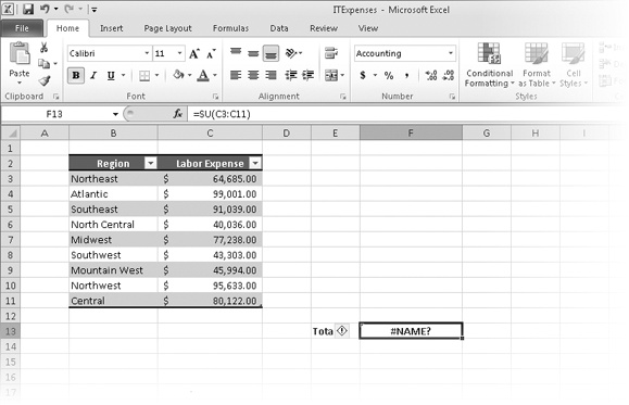
SET UP You need the ITExpenses_start workbook located in your Chapter10 practice file folder to complete this exercise. Open the ITExpenses_start workbook, and save it as ITExpenses. Then follow the steps.
If necessary, display the Summary worksheet. Then, in cell F9, type =C4, and press Enter.
The value $385,671.00 appears in cell F9.
Select cell F9 and type =SU.
Excel erases the existing formula, and Formula AutoComplete displays a list of possible functions to use in the formula.
In the Formula AutoComplete list, click SUM, and then press Tab.
Excel changes the contents of the formula bar to =SUM(.
Select the cell range C3:C8, type a right parenthesis ( ) ) to make the formula bar’s contents =SUM(C3:C8), and then press Enter.
The value $2,562,966.00 appears in cell F9.
In cell F10, type =SUM(C4:C5), and then press Enter.
Select cell F10, and then in the formula box, select the cell reference C4, and press F4.
Excel changes the cell reference to $C$4.
In the formula box, select the cell reference C5, press F4, and then press Enter.
Excel changes the cell reference to $C$5.
On the tab bar, click the JuneLabor sheet tab.
The JuneLabor worksheet opens.
In cell F13, type =SUM(J.
Excel displays JuneSummary, the name of the table in the JuneLabor worksheet.
Press Tab.
Excel extends the formula to read =SUM(JuneSummary.
Type [, and then in the Formula AutoComplete list, click Labor Expense, and press Tab.
Excel extends the formula to read =SUM(JuneSummary[Labor Expense.
Type ]) to complete the formula, and then press Enter.
The value $637,051.00 appears in cell F13.

Another use for formulas is to display messages when certain conditions are met. For instance, Consolidated Messenger’s Vice President of Marketing, Craig Dewar, might have agreed to examine the rates charged to corporate customers who were billed for more than $100,000 during a calendar year. This kind of formula is called a conditional formula; one way to create a conditional formula in Excel is to use the IF function. To create a conditional formula, you click the cell to hold the formula and open the Insert Function dialog box. From within the dialog box, click IF in the list of available functions, and then click OK. When you do, the Function Arguments dialog box opens.

When you work with an IF function, the Function Arguments dialog box has three boxes: Logical_test, Value_if_true, and Value_if_false. The Logical_test box holds the condition you want to check. If the customer’s year-to-date shipping bill appears in cell G8, the expression would be G8>100000.
Now you need to have Excel display messages that indicate whether Craig Dewar should evaluate the account for a possible rate adjustment. To have Excel print a message from an IF function, you enclose the message in quotes in the Value_if_true or Value_if_false box. In this case, you would type “High-volume shipper—evaluate for rate decrease.” in the Value_if_true box and “Does not qualify at this time.” in the Value_if_false box.
Excel also includes several other conditional functions you can use to summarize your data, shown in the following table.
You can use the IFERROR function to display a custom error message, instead of relying on the default Excel error messages to explain what happened. For example, you could use an IFERROR formula when looking up the CustomerID value from cell G8 in the Customers table by using the VLOOKUP function. One way to create such a formula is =IFERROR(VLOOKUP(G8,Customers,2,false),“Customer not found”). If the function finds a match for the CustomerID in cell G8, it displays the customer’s name; if it doesn’t find a match, it displays the text Customer not found.
Note
See Also For more information about the VLOOKUP function, refer to Microsoft Excel 2010 Step by Step, by Curtis Frye (Microsoft Press, 2010).
Just as the COUNTIF function counts the number of cells that meet a criterion and the SUMIF function finds the total of values in cells that meet a criterion, the AVERAGEIF function finds the average of values in cells that meet a criterion. To create a formula using the AVERAGEIF function, you define the range to be examined for the criterion, the criterion, and, if required, the range from which to draw the values. As an example, consider a worksheet that lists each customer’s ID number, name, state, and total monthly shipping bill.

If you want to find the average order of customers from the state of Washington (abbreviated in the worksheet as WA), you can create the formula =AVERAGEIF(D3:D6, “WA”, E3:E6).
The AVERAGEIFS, SUMIFS, and COUNTIFS functions extend the capabilities of the AVERAGEIF, SUMIF, and COUNTIF functions to allow for multiple criteria. If you want to find the sum of all orders of at least $100,000 placed by companies in Washington, you can create the formula =SUMIFS(E3:E6, D3:D6, “=WA”, E3:E6, “>=100000”).
The AVERAGEIFS and SUMIFS functions start with a data range that contains values that the formula summarizes; you then list the data ranges and the criteria to apply to that range. In generic terms, the syntax runs =AVERAGEIFS(data_range, criteria_range1, criteria1[,criteria_range2, criteria2…]). The part of the syntax in square brackets (which aren’t used when you create the formula) is optional, so an AVERAGEIFS or SUMIFS formula that contains a single criterion will work. The COUNTIFS function, which doesn’t perform any calculations, doesn’t need a data range—you just provide the criteria ranges and criteria. For example, you could find the number of customers from Washington who were billed at least $100,000 by using the formula =COUNTIFS(D3:D6, “=WA”, E3:E6, “>=100000”).
In this exercise, you’ll create a conditional formula that displays a message if a condition is true, find the average of worksheet values that meet one criterion, and find the sum of worksheet values that meet two criteria.
Note
SET UP You need the PackagingCosts_start workbook located in your Chapter10 practice file folder to complete this exercise. Open the PackagingCosts_start workbook, and save it as PackagingCosts. Then follow the steps.
In cell G3, type the formula =IF(F3>=35000, “Request discount”, “No discount available”), and press Enter.
Excel accepts the formula, which displays Request discount if the value in cell F3 is at least 35,000 and displays No discount available if not. The value Request discount appears in cell G3.
Click cell G3, and drag the fill handle down until it covers cell G14.
Excel copies the formula in cell G3 to cells G4:G14, adjusting the formula to reflect the cells’ addresses. The results of the copied formulas appear in cells G4:G14.
In cell I3, type the formula =AVERAGEIF(C3:C14, “=Box”, F3:F14), and press Enter.
The value $46,102.50, which represents the average cost per category of boxes, appears in cell I3.
In cell I6, type =SUMIFS(F3:F14, C3:C14, “=Envelope”, E3:E14, “=International”).
The value $45,753.00, which represents the total cost of all envelopes used for international shipments, appears in cell I6.

Including calculations in a worksheet gives you valuable answers to questions about your data. As is always true, however, it is possible for errors to creep into your formulas. With Excel, you can find the source of errors in your formulas by identifying the cells used in a given calculation and describing any errors that have occurred. The process of examining a worksheet for errors is referred to as auditing.
Excel identifies errors in several ways. The first way is to display an error code in the cell holding the formula generating the error.
When a cell with an erroneous formula is the active cell, an Error button is displayed next to it. Pointing to the Error button displays an arrow. Clicking the arrow displays a menu with options that provide information about the error and offer to help you fix it.
The following table lists the most common error codes and what they mean.
Another technique you can use to find the source of formula errors is to ensure that the appropriate cells are providing values for the formula. For example, you might want to calculate the total number of deliveries for a service level, but you could accidentally create a formula referring to the service levels’ names instead of their package quantities. You can identify the source of an error by having Excel trace a cell’s precedents, which are the cells with values used in the active cell’s formula. To do so, click the Formulas tab, and then in the Formula Auditing group, click Trace Precedents. When you do, Excel identifies those cells by drawing a blue tracer arrow from the precedents to the active cell.
You can also audit your worksheet by identifying cells with formulas that use a value from a given cell. For example, you might use one region’s daily package total in a formula that calculates the average number of packages delivered for all regions on a given day. Cells that use another cell’s value in their calculations are known as dependents, meaning that they depend on the value in the other cell to derive their own value. As with tracing precedents, you can click the Formulas tab, and then in the Formula Auditing group, click Trace Dependents.

If the cells identified by the tracer arrows aren’t the correct cells, you can hide the arrows and correct the formula. To hide the tracer arrows on a worksheet, display the Formulas tab, and then in the Formula Auditing group, click Remove Arrows.
If you prefer to have the elements of a formula error presented as text in a dialog box, you can use the Error Checking dialog box to view the error and the formula in the cell in which the error occurs. To display the Error Checking dialog box, display the Formulas tab, and then in the Formula Auditing group, click the Error Checking button. You can use the controls in the Error Checking dialog box to move through the formula one step at a time, to choose to ignore the error, or to move to the next or the previous error. If you click the Options button in the dialog box, you can also use the controls in the Excel Options dialog box to change how Excel determines what is an error and what isn’t.

Tip
If you clear the Formulas That Omit Cells In A Region check box, you can create formulas that don’t add up every value in a row, column, or range without Excel displaying an error.
For times when you just want to display the results of each step of a formula and don’t need the full power of the Error Checking tool, you can use the Evaluate Formula dialog box to move through each element of the formula. To display the Evaluate Formula dialog box, you display the Formulas tab and then, in the Formula Auditing group, click the Evaluate Formula button. The Evaluate Formula dialog box is much more useful for examining formulas that don’t produce an error but aren’t generating the result you expect.
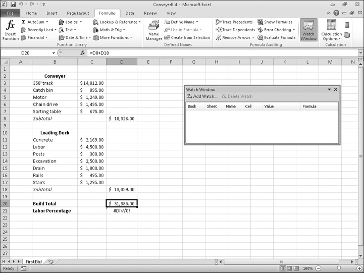
Finally, you can monitor the value in a cell regardless of where in your workbook you are by opening a Watch Window that displays the value in the cell. For example, if one of your formulas uses values from cells in other worksheets or even other workbooks, you can set a watch on the cell that contains the formula and then change the values in the other cells. To set a watch, click the cell you want to monitor, and then on the Formulas tab, in the Formula Auditing group, click Watch Window. Click Add Watch to have Excel monitor the selected cell.
As soon as you type in the new value, the Watch Window displays the new result of the formula. When you’re done watching the formula, select the watch, click Delete Watch, and close the Watch Window.
In this exercise, you’ll use the formula-auditing capabilities in Excel to identify and correct errors in a formula.
Note
SET UP You need the ConveyerBid_start workbook located in your Chapter10 practice file folder to complete this exercise. Open the ConveyerBid_start workbook, and save it as ConveyerBid. Then follow the steps.
Click cell D20.
 On the Formulas tab,
in the Formula Auditing group, click
Watch Window.
On the Formulas tab,
in the Formula Auditing group, click
Watch Window.The Watch Window opens.
Click Add Watch, and then in the Add Watch dialog box, click Add.
Cell D20 appears in the Watch Window.
Click cell D8.
 In the Formula
Auditing group, click the Trace
Precedents button.
In the Formula
Auditing group, click the Trace
Precedents button.A blue arrow begins at the cell range C3:C7 and points to cell D8.
 In the Formula
Auditing group, click the Remove
Arrows button.
In the Formula
Auditing group, click the Remove
Arrows button.The arrow disappears.
Click cell A1.
 In the Formula
Auditing group, click the Error
Checking button.
In the Formula
Auditing group, click the Error
Checking button.Click Next.
Excel displays a message box indicating that there are no more errors in the worksheet.
Click OK.
The message box and the Error Checking dialog box close.
In the Formula Auditing group, click the Error Checking arrow, and then in the list, click Trace Error.
Blue arrows appear, pointing to cell D21 from cells C12 and D19. These arrows indicate that using the values (or lack of values, in this case) in the indicated cells generates the error in cell D21.
In the Formula Auditing group, click Remove Arrows.
The arrows disappear.
In the formula box, delete the existing formula, type =C12/D20, and press Enter.
The value 14% appears in cell D21.
Click cell D21.
 In the Formula
Auditing group, click the Evaluate
Formula button.
In the Formula
Auditing group, click the Evaluate
Formula button.Click Evaluate three times to step through the formula’s elements, and then click Close.
The Evaluate Formula dialog box closes.
In the Watch Window, click the watch in the list.
Click Delete Watch.
The watch disappears.
On the Formulas tab, in the Formula Auditing group, click Watch Window.
The Watch Window closes.


You can add a group of cells to a formula by typing the formula, and then at the spot in the formula in which you want to name the cells, selecting the cells by using the mouse.
By creating named ranges, you can refer to entire blocks of cells with a single term, saving you lots of time and effort. You can use a similar technique with table data, referring to an entire table or one or more table columns.
When you write a formula, be sure you use absolute referencing ($A$1) if you want the formula to remain the same when it’s copied from one cell to another, or use relative referencing (A1) if you want the formula to change to reflect its new position in the worksheet.
Instead of typing a formula from scratch, you can use the Insert Function dialog box to help you on your way.
You can monitor how the value in a cell changes by adding a watch to the Watch Window.
To see which formulas refer to the values in the selected cell, use Trace Dependents; if you want to see which cells provide values for the formula in the active cell, use Trace Precedents.
You can step through the calculations of a formula in the Evaluate Formula dialog box or go through a more rigorous error-checking procedure by using the Error Checking tool.