
Chapter at a Glance
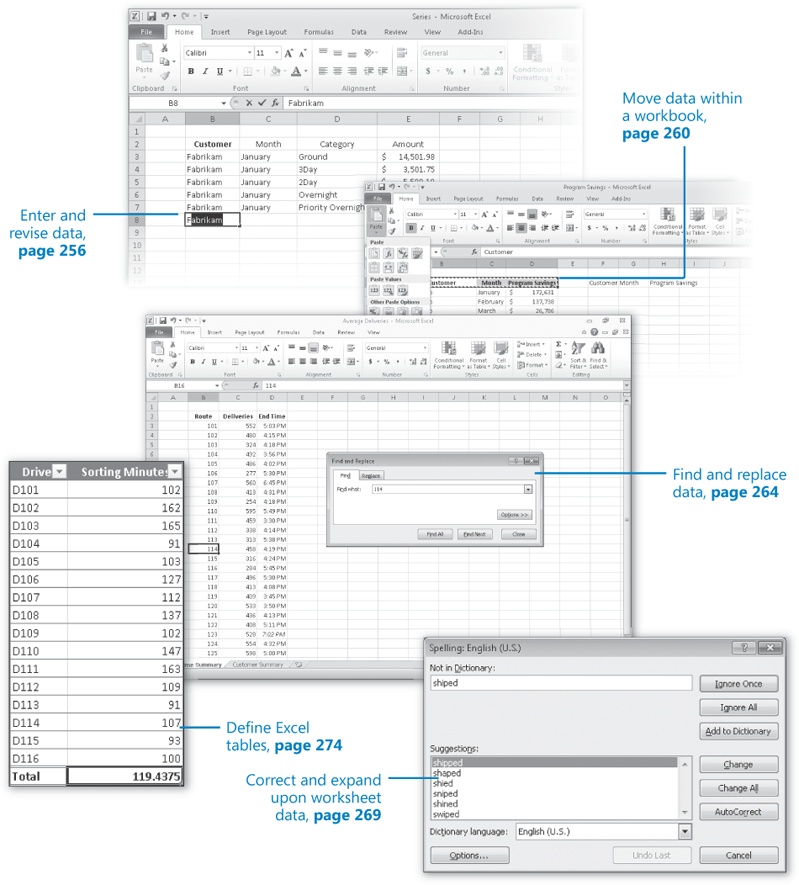
With Microsoft Excel 2010, you can visualize and present information effectively by using charts, graphics, and formatting, but the data is the most important part of any workbook. By learning to enter data efficiently, you will make fewer data entry errors and give yourself more time to analyze your data so you can make decisions about your organization’s performance and direction.
Excel provides a wide variety of tools you can use to enter and manage worksheet data effectively. For example, you can organize your data into Excel tables, which enables you to store and analyze your data quickly and efficiently. Also, you can enter a data series quickly, repeat one or more values, and control how Excel formats cells, columns, and rows moved from one part of a worksheet to another with a minimum of effort. With Excel, you can check the spelling of worksheet text, look up alternative words by using the Thesaurus, and translate words to foreign languages.
In this chapter, you’ll learn how to enter and revise Excel data, move data within a workbook, find and replace existing data, use proofing and reference tools to enhance your data, and organize your data by using Excel tables.
Note
Practice Files Before you can complete the exercises in this chapter, you need to copy the book’s practice files to your computer. The practice files you’ll use to complete the exercises in this chapter are in the Chapter09 practice file folder. A complete list of practice files is provided in Using the Practice Files at the beginning of this book.
After you create a workbook, you can begin entering data. The simplest way to enter data is to click a cell and type a value. This method works very well when you’re entering a few pieces of data, but it is less than ideal when you’re entering long sequences or series of values. For example, Craig Dewar, the Vice President of Marketing for Consolidated Messenger, might want to create a worksheet listing the monthly program savings that large customers can realize if they sign exclusive delivery contracts with Consolidated Messenger. To record those numbers, he would need to create a worksheet tracking each customer’s monthly program savings.

Repeatedly entering the sequence January, February, March, and so on can be handled by copying and pasting the first occurrence of the sequence, but there’s an easier way to do it: use AutoFill. With AutoFill, you enter the first element in a recognized series, click and hold the mouse button down on the fill handle at the lower-right corner of the cell, and drag the fill handle until the series extends far enough to accommodate your data. Using a similar tool, FillSeries, you can enter two values in a series and use the fill handle to extend the series in your worksheet. For example, if you want to create a series starting at 2 and increasing by 2, you can put 2 in the first cell and 4 in the second cell, select both cells, and then use the fill handle to extend the series to your desired end value.
You do have some control over how Excel extends the values in a series when you drag the fill handle. For example, if you drag the fill handle up (or to the left), Excel extends the series to include previous values. If you type January in a cell and then drag that cell’s fill handle up (or to the left), Excel places December in the first cell, November in the second cell, and so on.
Another way to control how Excel extends a data series is by holding down the Ctrl key while you drag the fill handle. For example, if you select a cell that contains the value January and then drag the fill handle down, Excel extends the series by placing February in the next cell, March in the cell after that, and so on. If you hold down the Ctrl key while you drag the fill handle, however, Excel repeats the value January in each cell you add to the series.
Tip
Be sure to experiment with how the fill handle extends your series and how pressing the Ctrl key changes that behavior. Using the fill handle can save you a lot of time entering data.
Other data entry techniques you’ll use in this section are AutoComplete, which detects when a value you’re entering is similar to previously entered values; Pick From Drop-Down List, from which you can choose a value from among the existing values in a column; and Ctrl+Enter, which you can use to enter a value in multiple cells simultaneously.
Note
Troubleshooting If an AutoComplete suggestion doesn’t appear as you begin typing a cell value, the option might be turned off. To turn on AutoComplete, click the File tab, and then click Options. In the Excel Options dialog box, display the Advanced page. In the Editing Options area of the page, select the Enable AutoComplete For Cell Values check box, and then click OK.
The following table summarizes these data entry techniques.
|
Method |
Action |
|---|---|
|
AutoFill |
Enter the first value in a recognized series and use the fill handle to extend the series. |
|
FillSeries |
Enter the first two values in a series and use the fill handle to extend the series. |
|
AutoComplete |
Type the first few letters in a cell, and if a similar value exists in the same column, Excel suggests the existing value. |
|
Right-click a cell, and then click Pick From Drop-Down List. A list of existing values in the cell’s column is displayed. Click the value you want to enter into the cell. | |
|
Ctrl+Enter |
Select a range of cells, each of which you want to contain the same data, type the data in the active cell, and press Ctrl+Enter. |
Another handy feature in Excel is the AutoFill Options button that appears next to data you add to a worksheet by using the fill handle.

Clicking the AutoFill Options button displays a list of actions Excel can take regarding the cells affected by your fill operation. The options in the list are summarized in the following table.
In this exercise, you’ll enter data by using multiple methods and control how Excel formats an extended data series.
Note
SET UP You need the Series_start workbook located in your Chapter09 practice file folder to complete this exercise. Start Excel, open the Series_start workbook, and save it as Series. Then follow the steps.
On the Monthly worksheet, select cell B3, and then drag the fill handle down until it covers cells B3:B7.
Excel repeats the value Fabrikam in cells B4:B7.
Select cell C3, hold down the Ctrl key, and drag the fill handle down until it covers cells C3:C7.
Excel repeats the value January in cells C4:C7.
Select cell B8, and then type the letter F.
Excel displays the characters abrikam in reverse colors.
Press Tab to accept the value Fabrikam for the cell.
In cell C8, type February.
Right-click cell D8, and then click Pick From Drop-down List.
From the list, click 2Day.
In cell E8, type 11802.14, and then press Tab or Enter.
Select cell B2, and then drag the fill handle so that it covers cells C2:E2.
Excel replaces the values in cells C2:E2 with the value Customer.
 Click the AutoFill
Options button, and then
click Fill Formatting Only.
Click the AutoFill
Options button, and then
click Fill Formatting Only.Excel restores the original values in cells C2:E2 but applies the formatting of cell B2 to those cells.


You can move to a specific cell in lots of ways, but the most direct method is to click the desired cell. The cell you click will be outlined in black, and its contents, if any, will appear in the formula bar. When a cell is outlined, it is the active cell, meaning that you can modify its contents. You use a similar method to select multiple cells (referred to as a cell range)—just click the first cell in the range, hold down the left mouse button, and drag the mouse pointer over the remaining cells you want to select. After you select the cell or cells you want to work with, you can cut, copy, delete, or change the format of the contents of the cell or cells. For instance, Gregory Weber, the Northwest Distribution Center Manager for Consolidated Messenger, might want to copy the cells that contain a set of column labels to a new page that summarizes similar data.
You’re not limited to selecting cells individually or as part of a range. For example, you might need to move a column of price data one column to the right to make room for a column of headings that indicate to which service category (ground, three-day express, two-day express, overnight, or priority overnight) a set of numbers belongs. To move an entire column (or entire columns) of data at a time, you click the column’s header, located at the top of the worksheet. Clicking a column header highlights every cell in that column and enables you to copy or cut the column and paste it elsewhere in the workbook. Similarly, clicking a row’s header highlights every cell in that row, enabling you to copy or cut the row and paste it elsewhere in the workbook.
When you copy a cell, cell range, row, or column, Excel copies the cells’ contents and formatting. In previous versions of Excel, you would paste the cut or copied items and then click the Paste Options button to select which aspects of the cut or copied cells to paste into the target cells. The problem with using the Paste Options button was that there was no way to tell what your pasted data would look like until you completed the paste operation. If you didn’t like the way the pasted data looked, you had to click the Paste Options button again and try another option.
With the new Paste Live Preview capability in Excel, you can see what your pasted data will look like without committing to the paste operation. To preview your data using Paste Live Preview, cut or copy worksheet data and then, on the Home tab of the ribbon, in the Clipboard group, click the Paste button’s arrow to display the Paste gallery, and point to one of the icons. When you do, If you position your mouse pointer over one icon in the Paste gallery and then move it over another icon without clicking, Excel will update the preview to reflect the new option. Depending on the cells’ contents, two or more of the paste options might lead to the same result.

Note
Troubleshooting If pointing to an icon in the Paste gallery doesn’t result in a live preview, that option might be turned off. To turn Paste Live Preview on, click the File tab and click Options to display the Excel Options dialog box. Click General, select the Enable Live Preview check box, and click OK.
After you click an icon to complete the paste operation, Excel displays the Paste Options button next to the pasted cells. Clicking the Paste Options button displays the Paste Options palette as well, but pointing to one of those icons doesn’t generate a preview. If you want to display Paste Live Preview again, you will need to press Ctrl+Z to undo the paste operation and, if necessary, cut or copy the data again to use the icons in the Home tab’s Clipboard group.
Note
Troubleshooting If the Paste Options button doesn’t appear, you can turn the feature on by clicking the File tab and then clicking Options to display the Excel Options dialog box. In the Excel Options dialog box, display the Advanced page and then, in the Cut, Copy, And Paste area, select the Show Paste Options Buttons When Content Is Pasted check box. Click OK to close the dialog box and save your setting.
After cutting or copying data to the Clipboard, you can access additional paste options from the Paste gallery and from the Paste Special dialog box, which you display by clicking Paste Special at the bottom of the Paste gallery.
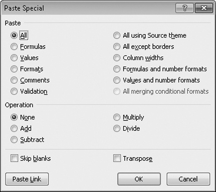
In the Paste Special dialog box, you can specify the aspect of the Clipboard contents you want to paste, restricting the pasted data to values, formats, comments, or one of several other options. You can perform mathematical operations involving the cut or copied data and the existing data in the cells you paste the content into. You can transpose data—change rows to columns and columns to rows—when you paste it, by clicking Transpose in the Paste gallery or by selecting the Transpose check box in the Paste Special dialog box.
In this exercise, you’ll copy a set of data headers to another worksheet, move a column of data within a worksheet, and use Paste Live Preview to control the appearance of copied data.
Note
SET UP You need the 2010Q1ShipmentsByCategory_start workbook located in your Chapter09 practice file folder to complete this exercise. Open the 2010Q1ShipmentsByCategory_start workbook, and save it as 2010Q1ShipmentsByCategory. Then follow the steps.
On the Count worksheet, select cells B2:D2.
 On the Home tab, in
the Clipboard group, click the Copy button.
On the Home tab, in
the Clipboard group, click the Copy button.Excel copies the contents of cells B2:D2 to the Clipboard.
On the tab bar, click the Sales tab to display that worksheet.
Select cell B2.
 On the Home tab, in
the Clipboard group, click the Paste button’s arrow, point to the
first icon in the Paste group, and then
click the Keep Source Formatting icon
(the final icon in the first row of the Paste gallery.)
On the Home tab, in
the Clipboard group, click the Paste button’s arrow, point to the
first icon in the Paste group, and then
click the Keep Source Formatting icon
(the final icon in the first row of the Paste gallery.)Excel displays how the data would look if you pasted the copied values without formatting, and then pastes the header values into cells B2:D2, retaining the original cells’ formatting.
Right-click the column header of column I, and then click Cut.
Excel outlines column I with a marquee.
Right-click the header of column E, and then, under Paste Options, click Paste.
Excel pastes the contents of column I into column E.
Note
Keyboard Shortcut Press Ctrl+V to paste worksheet contents exactly as they appear in the original cell.
Note
Troubleshooting The appearance of buttons and groups on the ribbon changes depending on the width of the program window. For information about changing the appearance of the ribbon to match our screen images, see Modifying the Display of the Ribbon at the beginning of this book.

Excel worksheets can hold more than one million rows of data, so in large data collections it’s unlikely that you would have the time to move through a worksheet one row at a time to locate the data you want to find. You can locate specific data in an Excel worksheet by using the Find And Replace dialog box, which has two pages (one named Find, the other named Replace) that you can use to search for cells that contain particular values. Using the controls on the Find page identifies cells that contain the data you specify; using the controls on the Replace page, you can substitute one value for another. For example, if one of Consolidated Messenger’s customers changes its company name, you can change every instance of the old name to the new name by using the Replace functionality.
When you need more control over the data that you find and replace, for instance, if you want to find cells in which the entire cell value matches the value you’re searching for, you can click the Options button to expand the Find And Replace dialog box.

One way you can use the extra options in the Find And Replace dialog box is to use a specific format to identify data that requires review. As an example, Consolidated Messenger’s Vice President of Marketing, Craig Dewar, could make corporate sales plans based on a projected budget for the next year and mark his trial figures using a specific format. After the executive board finalizes the numbers, he could use the Find Format capability in the Find And Replace dialog box to locate the old values and change them by hand.
The following table summarizes the Find And Replace dialog box controls’ functions.
To change a value by hand, select the cell, and then either type a new value in the cell or, in the formula bar, select the value you want to replace and type the new value. You can also double-click a cell and edit its contents within the cell.
In this exercise, you’ll find a specific value in a worksheet, replace every occurrence of a company name in a worksheet, and find a cell with a particular formatting.
Note
SET UP You need the AverageDeliveries_start workbook located in your Chapter09 practice file folder to complete this exercise. Open the AverageDeliveries_start workbook, and save it as AverageDeliveries. Then follow the steps.
If necessary, click the Time Summary sheet tab.
 On the Home tab, in
the Editing group, click Find & Select, and then click Find.
On the Home tab, in
the Editing group, click Find & Select, and then click Find.The Find And Replace dialog box opens with the Find tab displayed.
In the Find what field, type 114.
Excel highlights cell B16, which contains the value 114.
Delete the value in the Find what field, and then click the Options button.
The Find And Replace dialog box expands to display additional search options.
Click Format.
Click the Font tab.
In the Font style list, click Italic.
Click OK.
The Find Format dialog box closes.
Click Find Next.
Excel highlights cell D25.
Click Close.
The Find And Replace dialog box closes.
On the tab bar, click the Customer Summary sheet tab.
The Customer Summary worksheet is displayed.
On the Home tab, in the Editing group, click Find & Select, and then click Replace.
The Find And Replace dialog box opens with the Replace tab displayed.
Click the Format arrow to the right of the Find what field, and then in the list, click Clear Find Format.
The format displayed next to the Find What field disappears.
In the Find what field, type Contoso.
In the Replace with field, type Northwind Traders.
Click Replace All.
A message box appears, indicating that Excel made three replacements.
Click OK to close the message box.
Click Close.
The Find And Replace dialog box closes.


After you enter your data, you should take the time to check and correct it. You do need to verify visually that each piece of numeric data is correct, but you can make sure that your worksheet’s text is spelled correctly by using the Excel spelling checker. When the spelling checker encounters a word it doesn’t recognize, it highlights the word and offers suggestions representing its best guess of the correct word. You can then edit the word directly, pick the proper word from the list of suggestions, or have the spelling checker ignore the misspelling. You can also use the spelling checker to add new words to a custom dictionary so that Excel will recognize them later, saving you time by not requiring you to identify the words as correct every time they occur in your worksheets.
Tip
After you make a change in a workbook, you can usually remove the change as long as you haven’t closed the workbook. To undo a change, click the Undo button on the Quick Access Toolbar. If you decide you want to keep a change, you can use the Redo command to restore it.
If you’re not sure of your word choice, or if you use a word that is almost but not quite right for your intended meaning, you can check for alternative words by using the Thesaurus. Several other research tools are also available, such as the Bing decision engine and the Microsoft Encarta dictionary, to which you can refer as you create your workbooks. To display those tools, on the Review tab, in the Proofing group, click Research to display the Research task pane.

Finally, if you want to translate a word from one language to another, you can do so by selecting the cell that contains the value you want to translate, displaying the Review tab, and then, in the Language group, clicking Translate. The Research task pane opens (or changes if it’s already open) and displays controls you can use to select the original and destination languages.

Important
Excel translates a sentence by using word substitutions, which means that the translation routine doesn’t always pick the best word for a given context. The translated sentence might not capture your exact meaning.
In this exercise, you’ll check a worksheet’s spelling, add terms to a dictionary, search the Thesaurus for an alternative word, and translate a word from English into French.
Note
SET UP You need the ServiceLevels_start workbook located in your Chapter09 practice file folder to complete this exercise. Open the ServiceLevels_start workbook, and save it as ServiceLevels. Then follow the steps.
Verify that the word shipped is highlighted in the Suggestions pane, and then click Change.
Excel corrects the word and displays the next questioned word: withn.
Click Change.
Excel corrects the word and displays the next questioned word: TwoDay.
Excel adds the word to the dictionary and displays the next questioned word: ThreeDay.
Click Add to Dictionary.
Excel adds the word to the dictionary.
In the Spelling dialog box, click Close.
A message box indicates that the spelling check is complete.
Click OK to close the message box.
 On the Review tab,
in the Proofing group, click Thesaurus.
On the Review tab,
in the Proofing group, click Thesaurus.The Research task pane opens.
If necessary, in the From list, click English (U.S.).
In the To list, click French (France).
The Research task pane displays French words that mean overnight.


With Excel, you’ve always been able to manage lists of data effectively, enabling you to sort your worksheet data based on the values in one or more columns, limit the data displayed by using criteria (for example, show only those routes with fewer than 100 stops), and create formulas that summarize the values in visible (that is, unfiltered) cells. In Excel 2007, the Excel product team extended your ability to manage your data by introducing Excel tables. Excel 2010 offers you the same capability.

To create an Excel table, type a series of column headers in adjacent cells, and then type a row of data below the headers. Click any header or data cell into which you just typed, and then, on the Home tab, in the Styles group, click Format As Table. In the gallery that opens, click the table style you want to apply. In the Format As Table dialog box, verify that the cells in the Where Is The Data For Your Table? field reflect your current selection and that the My Table Has Headers check box is selected, and then click OK.
Excel can also create an Excel table from an existing cell range as long as the range has no blank rows or columns within the data and there is no extraneous data in cells immediately below or next to the list. To create the Excel table, click any cell in the range and then, on the Home tab, in the Styles group, click the Format As Table button and select a table style. If your existing data has formatting applied to it, that formatting remains applied to those cells when you create the Excel table. If you want Excel to replace the existing formatting with the Excel table’s formatting, right-click the table style you want to apply and then click Apply And Clear Formatting.
When you want to add data to an Excel table, click the rightmost cell in the bottom row of the Excel table and press the Tab key to create a new row. You can also select a cell in the row immediately below the last row in the table or a cell in the column immediately to the right of the table and type a value into the cell. After you enter the value and move out of the cell, the AutoCorrect Options action button appears. If you didn’t mean to include the data in the Excel table, you can click Undo Table AutoExpansion to exclude the cells from the Excel table. If you never want Excel to include adjacent data in an Excel table again, click Stop Automatically Expanding Tables.
Tip
To stop Table AutoExpansion before it starts, click the File tab, and then click Options. In the Excel Options dialog box, click Proofing, and then click the AutoCorrect Options button to display the AutoCorrect dialog box. Click the AutoFormat As You Type tab, clear the Include New Rows And Columns In Table check box, and then click OK twice.
You can add rows and columns to an Excel table, or remove them from an Excel table without deleting the cells’ contents, by dragging the resize handle at the Excel table’s lower-right corner. If your Excel table’s headers contain a recognizable series of values (such as Region1, Region2, and Region3), and you drag the resize handle to create a fourth column, Excel creates the column with the label Region4—the next value in the series.
Excel tables often contain data you can summarize by calculating a sum or average, or by finding the maximum or minimum value in a column. To summarize one or more columns of data, you can add a Total row to your Excel table.

When you add the Total row, Excel creates a formula that summarizes the values in the rightmost Excel table column. To change that summary operation, or to add a summary operation to any other cell in the Total row, click the cell, click the arrow that appears, and then click the summary operation you want to apply. Clicking the More Functions menu item displays the Insert Function dialog box, from which you can select any of the functions available in Excel.
Much as it does when you create a new worksheet, Excel gives your Excel tables generic names such as Table1 and Table2. You can change an Excel table’s name to something easier to recognize by clicking any cell in the table, clicking the Design contextual tab, and then, in the Properties group, editing the value in the Table Name box. Changing an Excel table name might not seem important, but it helps make formulas that summarize Excel table data much easier to understand. You should make a habit of renaming your Excel tables so you can recognize the data they contain.
Note
See Also For more information about using the Insert Function dialog box and about referring to tables in formulas, see Creating Formulas to Calculate Values in Chapter 10.
If for any reason you want to convert your Excel table back to a normal range of cells, click any cell in the Excel table and then, on the Design contextual tab, in the Tools group, click Convert To Range. When Excel displays a message box asking if you’re sure you want to convert the table to a range, click OK.
In this exercise, you’ll create an Excel table from existing data, add data to an Excel table, add a Total row, change the Total row’s summary operation, and rename the Excel table.
Note
SET UP You need the DriverSortTimes_start workbook located in your Chapter09 practice file folder to complete this exercise. Open the DriverSortTimes_start workbook, and save it as DriverSortTimes. Then follow the steps.
Select cell B2.
 On the Home tab, in
the Styles group, click Format as Table, and then select a table
style.
On the Home tab, in
the Styles group, click Format as Table, and then select a table
style.Verify that the range =$B$2:$C$17 is displayed in the Where is the data for your table? field and that the My table has headers check box is selected, and then click OK.
Excel creates an Excel table from your data and displays the Design contextual tab.
In cell B18, type D116, press Tab, type 100 in cell C18, and then press Enter.
Select a cell in the table. Then on the Design contextual tab, in the Table Style Options group, select the Total Row check box.
A Total row appears at the bottom of your Excel table.
Select cell C19, click the arrow that appears at the right edge of the cell, and then click Average.
Excel changes the summary operation to Average.
On the Design contextual tab, in the Properties group, type the value SortTimes in the Table Name field, and then press Enter.
 On the Quick Access Toolbar, click the Save button to save your work.


You can enter a series of data quickly by typing one or more values in adjacent cells, selecting the cells, and then dragging the fill handle. To change how dragging the fill handle extends a data series, hold down the Ctrl key.
Dragging a fill handle displays the Auto Fill Options button, which you can use to specify whether to copy the selected cells’ values, extend a recognized series, or apply the selected cells’ formatting to the new cells.
With Excel, you can enter data by using a list, AutoComplete, or Ctrl+Enter. You should experiment with these techniques and use the one that best fits your circumstances.
When you copy (or cut) and paste cells, columns, or rows, you can use the new Paste Live Preview capability to preview how your data will appear before you commit to the paste operation.
After you paste cells, rows, or columns into your worksheet, Excel displays the Paste Options action button. You can use its controls to change which aspects of the cut or copied elements Excel applies to the pasted elements.
By using the options in the Paste Special dialog box, you can paste only specific aspects of cut or copied data, perform mathematical operations, transpose data, or delete blank cells when pasting.
You can find and replace data within a worksheet by searching for specific values or by searching for cells that have a particular format applied.
Excel provides a variety of powerful proofing and research tools, enabling you to check your workbook’s spelling, find alternative words by using the Thesaurus, and translate words between languages.
With Excel tables, you can organize and summarize your data effectively.