
8.5. OBSERVABILITY
In order to introduce the concept of observability [2−4], let us again consider the simple open-loop system illustrated in Figure 8.13. A system is completely observable if, given the control and the output over the interval t0 ![]() t
t ![]() T, one can determine the initial state x(t0). Qualitatively, the system G is observable if every state variable of G affects some of the outputs in c. It is very often desirable to determine information regarding the system states based on measurements of c. However, if we cannot observe one or more of the states from the measurements of c, then the system is not completely observable. We had assumed the systems were observable in our discussion of pole placement using linear-state variable feedback in Sections 8.2 and 8.3.
T, one can determine the initial state x(t0). Qualitatively, the system G is observable if every state variable of G affects some of the outputs in c. It is very often desirable to determine information regarding the system states based on measurements of c. However, if we cannot observe one or more of the states from the measurements of c, then the system is not completely observable. We had assumed the systems were observable in our discussion of pole placement using linear-state variable feedback in Sections 8.2 and 8.3.
A. Observability by Inspection
An an example of a system which is not completely observable, let us consider the signal-flow diagram illustrated in Figure 8.15. This system contains four states, only two of which are observable. The states x3(t) and x4(t) are not connected to the output c(t) in any manner. Therefore, x3(t) and x4(t) are not observable and the system is not completely observable.
B. The Observability Matrix
Let us now consider this problem more precisely and establish a mathematical criterion for determining whether a system is completely observable. Again, we limit our discussion to linear constant systems of the form
where x is an m × 1 vector, P is an m × m matrix, u is an r × 1 vector, B is an m × r matrix, c is a p × 1 vector, and L is a p × m matrix. The solution of Eq (8.69) is given by [see Eq. (2.265)]
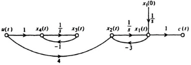
Figure 8.15 Signal-flow graph of a system that is not completely observable.
It will now be shown that observability depends on the matrices P and L. Substituting Eq (8.71) into Eq (8.70), we obtain
From the definition of observability we can see that the observability of x(t0) depends on the term LΦ(t − t0)x(t0). Therefore, the output c(t) when u = 0 is given by
Substituting Eq (8.60) into Eq (8.73), we obtain the following expression for the output c(t):
Equation (8.74) indicates that if the output c(t) is known over the time interval t0 ![]() t
t ![]() T, then x(t0) is uniquely determined from this equation if x(t0) is a linear combination of (LjPn)T for n = 0, 1, 2,..., m − 1, and j = 1, 2, 3,..., r. The matrix Lj is the 1 × m matrix formed by the elements of the jth row of L. Because (LjPn)T =
T, then x(t0) is uniquely determined from this equation if x(t0) is a linear combination of (LjPn)T for n = 0, 1, 2,..., m − 1, and j = 1, 2, 3,..., r. The matrix Lj is the 1 × m matrix formed by the elements of the jth row of L. Because (LjPn)T = ![]() , we let U be the m × mr matrix defined by
, we let U be the m × mr matrix defined by
The observability criterion states that the system is completely observable if there is a set of m linearly independent column vectors in the observability matrix U.
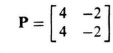
In order to illustrate the observability concept mathematically, consider a second-order system where
![]()
and
L = [1 0].
Therefore,
![]()
and
![]()
Substituting these values into Eq (8.75), we obtain
![]()
Because U is singular, the sytem is not completely observable.
As a second example, consider the second-order system where
and
L = [1 1].
Therefore,
![]()
and
![]()
Substituting these values into Eq (8.75), we obtain
![]()
Because U has two independent columns, the system is completely observable.