
2 Basic Workbook Skills
Introduction
Creating a Microsoft Excel workbook is as easy as entering data in the cells of an Excel worksheet. Each cell has a cell address which is made up of its column and row intersection. Cells on a worksheet contain either labels or values, a formula or remain blank. Cell entries can be modified using the keyboard or mouse. You can select cells in ranges that are contiguous (selected cells are adjacent to each other) or noncontiguous (selected cells are in different parts of the worksheet). Selected cells are used in formulas, to copy and paste data, to AutoFill, to apply date and time and other formatting functions.
In addition, Excel offers a Find and Replace feature that allows you to look for labels and values and make changes as necessary. When you need to spell check your worksheet, Excel can check and suggest spelling corrections. You can even customize the spelling dictionary by adding company specific words into AutoCorrect so that the spell checker doesn’t think it’s a misspelled word. The Actions feature works with other Microsoft Office programs to enhance your worksheets. Contact information can be pulled from your address book in Outlook, to your worksheet in Excel. Stock symbols can trigger a Smart Tag choice to import data on a publicly traded company. Additional research and language tools area available to build up the content of your workbooks.
If you accidentally make a change to a cell, you can use the Undo feature to remove, or “undo,” your last change. Excel remembers your recent changes to the worksheet, and gives you the opportunity to undo them. If you decide to Redo the Undo, you can erase the previous change. This is useful when moving, copying, inserting and deleting cell contents.
Making Label Entries
There are three basic types of cell entries: labels, values, and formulas. A label is text in a cell that identifies the data on the worksheet so readers can interpret the information. Excel does not use labels in its calculations. For example, the label price is used as a column header to identify the price of each item in the column. A value is a number you enter in a cell. Excel knows to include values in its calculations. To quickly and easily enter values, you can format a cell, a range of cells, or a column with a specific number-related format. Then, as you type, the cells are automatically formatted.
To perform a calculation in a worksheet, you enter a formula in a cell. A formula is a calculation that contains cell references, values, and arithmetic operators. The result of a formula appears in the worksheet cell where you entered the formula. The contents of the cell appears on the formula bar. Entering cell references rather than actual values in a formula has distinct advantages. When you change the data in the worksheet or copy the formula to other cells (copying this formula to the cell below), Excel automatically adjusts the cell references in the formula and returns the correct results.

Selecting Cells
In order to work with a cell—to enter data in it, edit or move it, or perform an action—you select the cell so it becomes the active cell. When you want to work with more than one cell at a time—to move or copy them, use them in a formula, or perform any group action—you must first select the cells as a range. A range can be contiguous (where selected cells are adjacent to each other) or non-contiguous (where the cells may be in different parts of the worksheet and are not adjacent to each other). As you select a range, you can see the range reference in the Name box. A range reference contains the cell address of the top-left cell in the range, a colon (:), and the cell address of the bottom-right cell in the range.
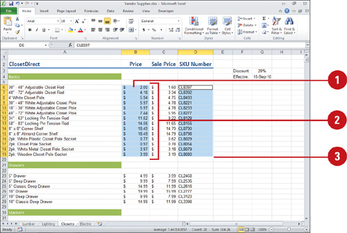
Select a Contiguous Range
![]() Click the first cell that you want to include in the range.
Click the first cell that you want to include in the range.
![]() Drag the mouse to the last cell you want to include in the range.
Drag the mouse to the last cell you want to include in the range.
TIMESAVER Instead of dragging, hold down the Shift key, and then click the lower-right cell in the range.
When a range is selected, the top-left cell is surrounded by the cell pointer, while the additional cells are selected.

Select a Non-contiguous Range
![]() Click the first cell you want to include in the range.
Click the first cell you want to include in the range.
![]() Drag the mouse to the last contiguous cell, and then release the mouse button.
Drag the mouse to the last contiguous cell, and then release the mouse button.
![]() Press and hold Ctrl, and then click the next cell or drag the pointer over the next group of cells you want in the range.
Press and hold Ctrl, and then click the next cell or drag the pointer over the next group of cells you want in the range.
To select more, repeat step 3 until all non-contiguous ranges are selected.
Selecting Rows, Columns, and Special Ranges
In addition to selecting a range of contiguous and non-contiguous cells in a single worksheet, you may need to select entire rows and columns, or even a range of cells across multiple worksheets. Cells can contain many different types of data, such as comments, constants, formulas, or conditional formats. Excel provides an easy way to locate these and many other special types of cells with the Go To Special dialog box. For example, you can select the Row Differences or Column Differences option to select cells that are different from other cells in a row or column, or select the Dependents option to select cells with formulas that refer to the active cell.
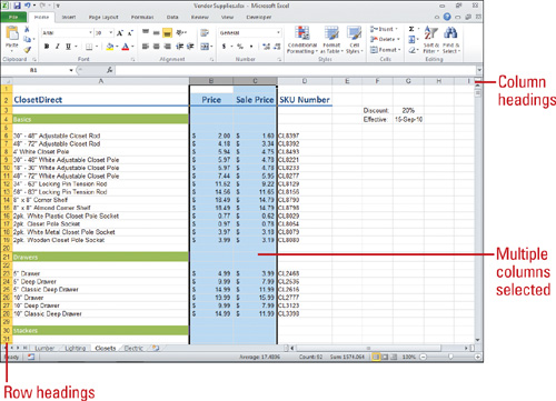
Select an Entire Rows or Columns
![]() To select a single row or column, click in the row or column heading, or select any cell in the row or column, and press Shift+spacebar.
To select a single row or column, click in the row or column heading, or select any cell in the row or column, and press Shift+spacebar.
![]() To select multiple adjacent rows or columns, drag in the row or column headings.
To select multiple adjacent rows or columns, drag in the row or column headings.
![]() To select multiple nonadjacent rows or columns, press Ctrl while you click the borders for the rows or columns you want to include.
To select multiple nonadjacent rows or columns, press Ctrl while you click the borders for the rows or columns you want to include.
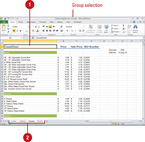
Select Multisheet Ranges
![]() Select the range in one sheet.
Select the range in one sheet.
![]() Select the worksheets to include in the range.
Select the worksheets to include in the range.
To select contiguous worksheets, press Shift and click the last sheet tab you want to include. To select non-contiguous worksheets, press Ctrl and click the sheets you want.
When you make a worksheet selection, Excel enters Group mode.
![]() To exit Group mode, click any sheet tab.
To exit Group mode, click any sheet tab.
Make Special Range Selections
![]() If you want to make a selection from within a range, select the range you want.
If you want to make a selection from within a range, select the range you want.
![]() Click the Home tab.
Click the Home tab.
![]() Click the Find & Select button, and then click Go To Special.
Click the Find & Select button, and then click Go To Special.
TIMESAVER Press F5 to open the Go To Special dialog box.
![]() Select the option in which you want to make a selection. When you click the Formulas option, select or clear the formula related check boxes.
Select the option in which you want to make a selection. When you click the Formulas option, select or clear the formula related check boxes.
![]() Click OK.
Click OK.
If no cells are found, Excel displays a message.

Entering Labels on a Worksheet
Labels turn a worksheet full of numbers into a meaningful report by identifying the different types of information it contains. You use labels to describe the data in worksheet cells, columns, and rows. You can enter a number as a label (for example, the year 2010), so that Excel does not use the number in its calculations. To help keep your labels consistent, you can use Excel’s AutoComplete feature, which automatically completes your entries (excluding numbers, dates, or times) based on previously entered labels.
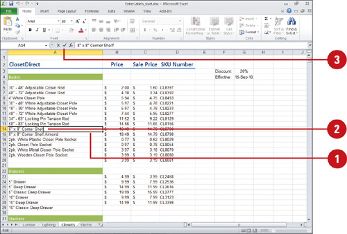
Enter a Text Label
![]() Click the cell where you want to enter a label.
Click the cell where you want to enter a label.
![]() Type a label. A label can include uppercase and lowercase letters, spaces, punctuation, and numbers.
Type a label. A label can include uppercase and lowercase letters, spaces, punctuation, and numbers.
![]() Press Enter, or click the Enter button on the formula bar.
Press Enter, or click the Enter button on the formula bar.
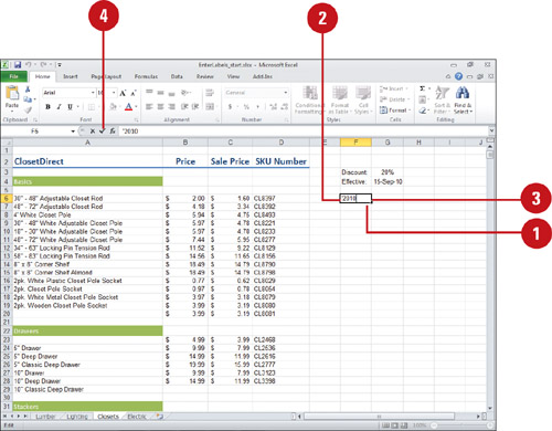
Enter a Number as a Label
![]() Click the cell where you want to enter a number as a label.
Click the cell where you want to enter a number as a label.
![]() Type ’(an apostrophe). The apostrophe is a label prefix and does not appear on the worksheet.
Type ’(an apostrophe). The apostrophe is a label prefix and does not appear on the worksheet.
![]() Type a number value.
Type a number value.
![]() Press Enter, or click the Enter button on the formula bar.
Press Enter, or click the Enter button on the formula bar.
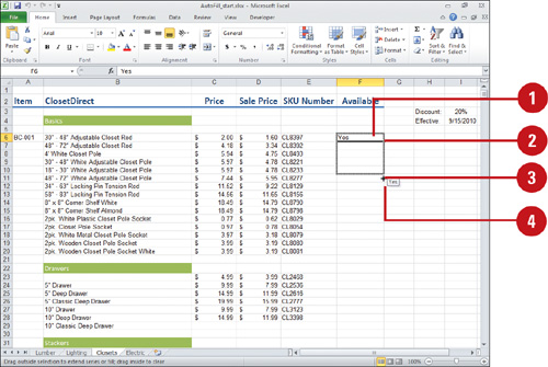
Enter a Label Using AutoComplete
![]() Type the first few characters of a label.
Type the first few characters of a label.
If Excel recognizes the entry, AutoComplete completes it.
![]() To accept the suggested entry, press Enter or click the Enter button on the formula bar.
To accept the suggested entry, press Enter or click the Enter button on the formula bar.
![]() To reject the suggested completion, simply continue typing.
To reject the suggested completion, simply continue typing.

Entering Values on a Worksheet
You can enter values as whole numbers, decimals, percentages, or dates using the numbers on the top row of your keyboard, or by pressing your Num Lock key, the numeric keypad on the right. When you enter a date or the time of day, Excel automatically recognizes these entries (if entered in an acceptable format) as numeric values and changes the cell’s format to a default date or time format. You can also change the way values, dates or times of day are shown.
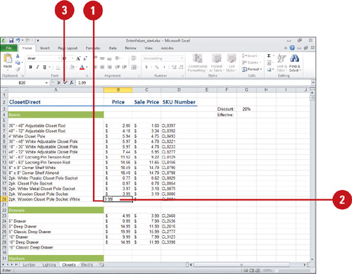
Enter a Value
![]() Click the cell where you want to enter a value.
Click the cell where you want to enter a value.
![]() Type a value.
Type a value.
![]() Press Enter, or click the Enter button on the formula bar.
Press Enter, or click the Enter button on the formula bar.
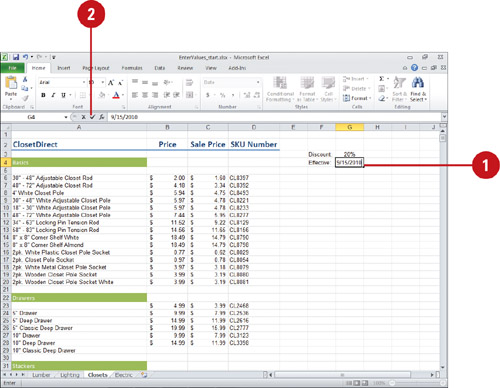
Enter a Date or Time
![]() To enter a date, type the date using a slash (/) or a hyphen (-) between the month, day, and year in a cell or on the formula bar.
To enter a date, type the date using a slash (/) or a hyphen (-) between the month, day, and year in a cell or on the formula bar.
To enter a time, type the hour based on a 12-hour clock, followed by a colon (:), followed by the minute, followed by a space, and ending with an “a” or a “p” to denote A.M. or P.M.
![]() Press Enter, or click the Enter button on the formula bar.
Press Enter, or click the Enter button on the formula bar.
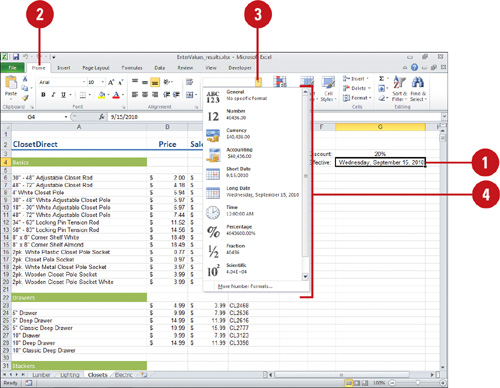
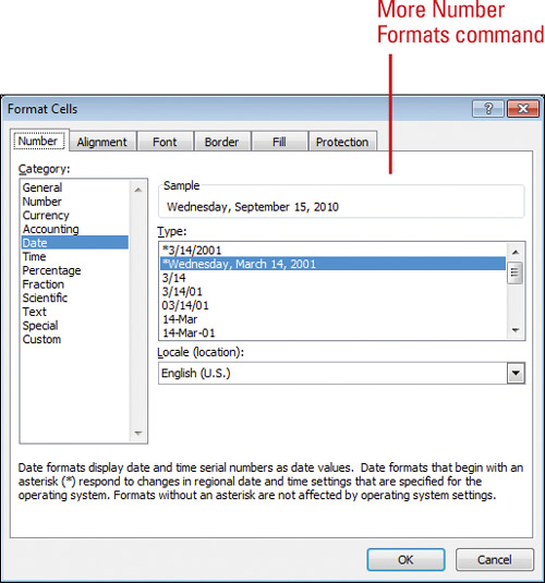
Format Values Quickly
![]() Click the cell that contains the date format you want to change.
Click the cell that contains the date format you want to change.
![]() Click the Home tab.
Click the Home tab.
![]() Click the Number Format list arrow.
Click the Number Format list arrow.
![]() Click the number format you want, which includes:
Click the number format you want, which includes:
![]() General. No specific format.
General. No specific format.
![]() Number. 38873.00
Number. 38873.00
![]() Currency.$38,873.00
Currency.$38,873.00
![]() Accounting.$ 38,873.00
Accounting.$ 38,873.00
![]() Short Date. 9/15/2010
Short Date. 9/15/2010
![]() Long Date. Wednesday, September 15, 2010
Long Date. Wednesday, September 15, 2010
![]() Time. 12:00:00 AM
Time. 12:00:00 AM
![]() Percentage. 38873.00%
Percentage. 38873.00%
![]() Fraction. 38873
Fraction. 38873
![]() Scientific. 3.89E+04
Scientific. 3.89E+04
![]() More Number Formats. Opens the Format Cell dialog box, where you can format cells with multiple options at one time.
More Number Formats. Opens the Format Cell dialog box, where you can format cells with multiple options at one time.
Entering Values Quickly with AutoFill
AutoFill is a feature that automatically fills in data based on the data in adjacent cells. Using the fill handle, you can enter data in a series, or you can copy values or formulas to adjacent cells. A single cell entry can result in a repeating value or label, or the results can be a more complex series. You can enter your value or label, and then complete entries such as days of the week, weeks of the year, months of the year, or consecutive numbering.
Enter Repeating Data Using AutoFill
![]() Select the first cell in the range you want to fill.
Select the first cell in the range you want to fill.
![]() Enter the starting value to be repeated.
Enter the starting value to be repeated.
![]() Position the pointer on the lower-right corner of the selected cell. The pointer changes to the fill handle (a black plus sign).
Position the pointer on the lower-right corner of the selected cell. The pointer changes to the fill handle (a black plus sign).
![]() Drag the fill handle over the range you want the value repeated.
Drag the fill handle over the range you want the value repeated.
![]() To choose how to fill the selection, click the AutoFill Options button, and then click the option you want.
To choose how to fill the selection, click the AutoFill Options button, and then click the option you want.
Create a Complex Series Using AutoFill
![]() Enter the starting value for the series, and then press Enter.
Enter the starting value for the series, and then press Enter.
![]() Select the first cell in the range you want to fill.
Select the first cell in the range you want to fill.
![]() Position the pointer on the lower-right corner of the selected cell. The pointer changes to the fill handle (a black plus sign).
Position the pointer on the lower-right corner of the selected cell. The pointer changes to the fill handle (a black plus sign).
![]() Drag the fill handle over the range you want the value repeated.
Drag the fill handle over the range you want the value repeated.
![]() To choose how to fill the selection, click the AutoFill Options button, and then click the option you want.
To choose how to fill the selection, click the AutoFill Options button, and then click the option you want.

Fill with Contents of Adjacent Cells
![]() Select the cell below, to the right, above, or to the left of the cell that contains the data you want to fill.
Select the cell below, to the right, above, or to the left of the cell that contains the data you want to fill.
![]() Click the Home tab.
Click the Home tab.
![]() Click the Fill button, and then click Down, Right, Up or Left.
Click the Fill button, and then click Down, Right, Up or Left.
TIMESAVER To quickly fill a cell with the contents of the cell above or to the left of it, press Ctrl+D or Ctrl+R.

Create a Custom Fill
![]() If you want to use an existing list, select the list of items.
If you want to use an existing list, select the list of items.
![]() Click the File tab, and then click Options.
Click the File tab, and then click Options.
![]() In the left pane, click Advanced.
In the left pane, click Advanced.
![]() Click Edit Custom Lists.
Click Edit Custom Lists.
![]() Click the option you want.
Click the option you want.
![]() New list. Click NEW LIST, type the entries you want, press Enter after each. Click Add.
New list. Click NEW LIST, type the entries you want, press Enter after each. Click Add.
![]() Existing list. Verify the cell reference of the selected list appears in the Import list, and then click Import.
Existing list. Verify the cell reference of the selected list appears in the Import list, and then click Import.
![]() Click OK, and then click OK again.
Click OK, and then click OK again.

Editing Cell Contents
Even if you plan ahead, you can count on having to make changes on a worksheet. Sometimes it’s because you want to correct an error. Other times it’s because you want to see how your worksheet results would be affected by different conditions, such as higher sales, fewer units produced, or other variables. You can edit data just as easily as you enter it, using the formula bar or directly editing the active cell.
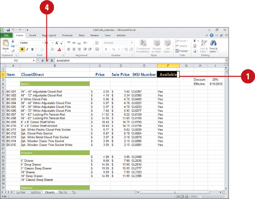
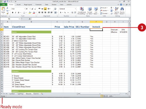
Edit Cell Contents
![]() Double-click the cell you want to edit. The insertion point appears in the cell.
Double-click the cell you want to edit. The insertion point appears in the cell.
The Status bar now displays Edit instead of Ready.
![]() If necessary, use the Home, End, and arrow keys to position the insertion point within the cell contents.
If necessary, use the Home, End, and arrow keys to position the insertion point within the cell contents.
![]() Use any combination of the Backspace and Delete keys to erase unwanted characters, and then type new characters as needed.
Use any combination of the Backspace and Delete keys to erase unwanted characters, and then type new characters as needed.
![]() Click the Enter button on the formula bar to accept the edit, or click the Esc button to cancel the edit.
Click the Enter button on the formula bar to accept the edit, or click the Esc button to cancel the edit.
The Status bar now displays Ready instead of Edit.
Clearing Cell Contents
You can clear a cell to remove its contents. Clearing a cell does not remove the cell from the worksheet; it just removes from the cell whatever elements you specify: data, comments (also called cell notes), or formatting instructions. When clearing a cell, you must specify whether to remove one, two, or all three of these elements from the selected cell or range.
Clear Cell Contents, Formatting, and Comments
![]() Select the cell or range you want to clear.
Select the cell or range you want to clear.
![]() Click the Home tab.
Click the Home tab.
![]() Click the Clear button, and then click any of the following options:
Click the Clear button, and then click any of the following options:
![]() Clear All. Clears contents and formatting.
Clear All. Clears contents and formatting.
![]() Clear Formats. Clears formatting and leaves contents.
Clear Formats. Clears formatting and leaves contents.
![]() Clear Contents. Clears contents and leaves formatting.
Clear Contents. Clears contents and leaves formatting.
![]() Clear Comments. Clears comments; removes purple triangle indicator.
Clear Comments. Clears comments; removes purple triangle indicator.
TIMESAVER To quickly clear contents, select the cell or range you want to clear, right-click the cell or range, and then click Clear Contents, or press Delete.

Understanding How Excel Pastes Data
If you want to use data that has already been entered on your worksheet, you can cut or copy it, and then paste it in another location. When you cut or copy data, the data is stored in an area of memory called the Clipboard. When pasting a range of cells from the Clipboard, you only need to specify the first cell in the new location. After you select the first cell in the new location and then click the Paste button, Excel automatically places all the selected cells in the correct order. Depending on the number of cells you select before you cut or copy, Excel pastes data in one of the following ways:
![]() One to one. A single cell in the Clipboard is pasted to one cell location.
One to one. A single cell in the Clipboard is pasted to one cell location.
![]() One to many. A single cell in the Clipboard is pasted into a selected range of cells.
One to many. A single cell in the Clipboard is pasted into a selected range of cells.
![]() Many to one. Many cells are pasted into a range of cells, but only the first cell is identified. The entire contents of the Clipboard will be pasted starting with the selected cell. Make sure there is enough room for the selection; if not, the selection will copy over any previously occupied cells.
Many to one. Many cells are pasted into a range of cells, but only the first cell is identified. The entire contents of the Clipboard will be pasted starting with the selected cell. Make sure there is enough room for the selection; if not, the selection will copy over any previously occupied cells.
![]() Many to many. Many cells are pasted into a range of cells. The entire contents of the Clipboard will be pasted into the selected cells. If the selected range is larger than the selection, the data will be repeated in the extra cells. To turn off the selection marquee and cancel your action, press the Esc key.
Many to many. Many cells are pasted into a range of cells. The entire contents of the Clipboard will be pasted into the selected cells. If the selected range is larger than the selection, the data will be repeated in the extra cells. To turn off the selection marquee and cancel your action, press the Esc key.

Storing Cell Contents
With Microsoft Office, you can use the Office Clipboard to store multiple pieces of information from several different sources in one storage area shared by all Office programs. Unlike the Clipboard, which only stores a single piece of information at a time, the Office Clipboard allows you to copy text or pictures from one or more files. When you copy multiple items, you see the Office Clipboard, showing all the items you stored there. You can paste these pieces of information into any Office program, either individually or all at once.
Copy and Paste Data to the Office Clipboard
![]() Click the Home tab.
Click the Home tab.
![]() Click the Clipboard Dialog Box Launcher.
Click the Clipboard Dialog Box Launcher.
![]() Select the data you want to copy.
Select the data you want to copy.
![]() Click the Copy button.
Click the Copy button.
The data is copied into the first empty position on the Clipboard task pane.
![]() Click the first cell or range where you want to paste data.
Click the first cell or range where you want to paste data.
![]() Click the Office Clipboard item you want to paste, or point to the item, click the list arrow, and then click Paste.
Click the Office Clipboard item you want to paste, or point to the item, click the list arrow, and then click Paste.
![]() Click the Close button in the task pane.
Click the Close button in the task pane.

Copying Cell Contents
You can copy and move data on a worksheet from one cell or range to another location on any worksheet in your workbook. When you copy data, a duplicate of the selected cells is placed on the Clipboard. To complete the copy or move, you must paste the data stored on the Clipboard in another location. The Paste live preview (New!) allows you to view your paste results before you actually paste it. With the Paste Special command, you can control what you want to paste and even perform mathematical operations. To copy or move data without using the Clipboard, you can use a technique called drag-and-drop. Drag-and-drop makes it easy to copy or move data short distances on your worksheet.
Copy Data Using the Clipboard
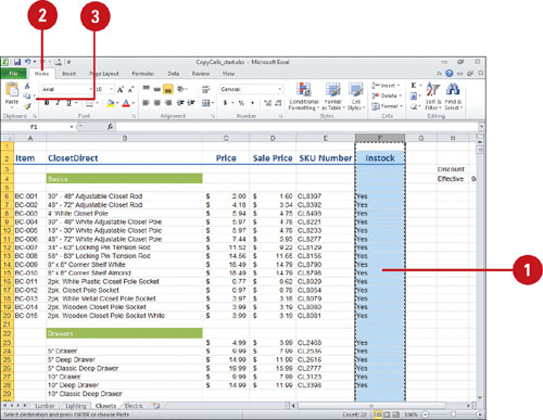
![]() Select the cell or range that contains the data you want to copy.
Select the cell or range that contains the data you want to copy.
![]() Click the Home tab.
Click the Home tab.
![]() Click the Copy button.
Click the Copy button.
The data in the cells remains in its original location and an outline of the selected cells, called a marquee, shows the size of the selection. If you don’t want to paste this selection, press Esc to remove the marquee.
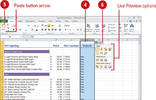
![]() Click the first cell or range where you want to paste the data.
Click the first cell or range where you want to paste the data.
![]() Click the Paste button or click the Paste button arrow, point to an option to display a live preview (New!) of the paste, and then click to paste the item.
Click the Paste button or click the Paste button arrow, point to an option to display a live preview (New!) of the paste, and then click to paste the item.
When you point to a paste option for the live preview, use the ScreenTip to determine the option.
If you don’t want to paste this selection anywhere else, press Esc to remove the marquee.
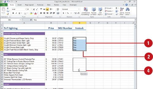
![]() If you want to change the way the data pastes into the document, click the Paste Options button, point to an option for the live preview (New!), and then select the option you want.
If you want to change the way the data pastes into the document, click the Paste Options button, point to an option for the live preview (New!), and then select the option you want.
Copy Data Using Drag-and-Drop
![]() Select the cell or range that contains the data you want to copy.
Select the cell or range that contains the data you want to copy.
![]() Move the mouse pointer to an edge of the selected cell or range until the pointer changes to an arrowhead.
Move the mouse pointer to an edge of the selected cell or range until the pointer changes to an arrowhead.
![]() Press and hold the mouse button and Ctrl.
Press and hold the mouse button and Ctrl.
![]() Drag the selection to the new location, and then release the mouse button and Ctrl.
Drag the selection to the new location, and then release the mouse button and Ctrl.
Paste Data with Special Results
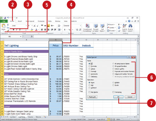
![]() Select the cell or range that contains the data you want to copy.
Select the cell or range that contains the data you want to copy.
![]() Click the Home tab.
Click the Home tab.
![]() Click the Copy button.
Click the Copy button.
![]() Click the first cell or range where you want to paste the data.
Click the first cell or range where you want to paste the data.
![]() Click the Paste button, and then click Paste Special.
Click the Paste button, and then click Paste Special.
![]() Click the option buttons with the paste results and mathematical operations you want.
Click the option buttons with the paste results and mathematical operations you want.
![]() Click OK.
Click OK.
Moving Cell Contents
Unlike copied data, moved data no longer remains in its original location. Perhaps you typed data in a range of cells near the top of a worksheet, but later realized it should appear near the bottom of the sheet. Moving data lets you change its location without having to retype it. When you move data, you are cutting the data from its current location and pasting it elsewhere. Cutting removes the selected cell or range content from the worksheet and places it on the Clipboard. The Paste live preview (New!) allows you to view your paste results before you actually paste it.
Move Data Using the Clipboard
![]() Select the cell or range that contains the data you want to move.
Select the cell or range that contains the data you want to move.
![]() Click the Home tab.
Click the Home tab.
![]() Click the Cut button.
Click the Cut button.
An outline of the selected cells, called a marquee, shows the size of the selection. If you don’t want to paste this selection, press Esc to remove the marquee.
![]() Click the top-left cell of the range where you want to paste the data.
Click the top-left cell of the range where you want to paste the data.
![]() Click the Paste button or click the Paste button arrow, point to an option to display a live preview (New!) of the paste, and then click to paste the item.
Click the Paste button or click the Paste button arrow, point to an option to display a live preview (New!) of the paste, and then click to paste the item.
The marquee disappears. The data is still on the Clipboard and still available for further pasting until you replace it with another selection.

Move Data Using Drag-and-Drop
![]() Select the cell or range that contains the data you want to move.
Select the cell or range that contains the data you want to move.
![]() Move the mouse pointer to an edge of the cell until the pointer changes to an arrowhead.
Move the mouse pointer to an edge of the cell until the pointer changes to an arrowhead.
![]() Press and hold the mouse button while dragging the selection to its new location, and then release the mouse button.
Press and hold the mouse button while dragging the selection to its new location, and then release the mouse button.
Paste Cells from Rows to Columns or Columns to Rows
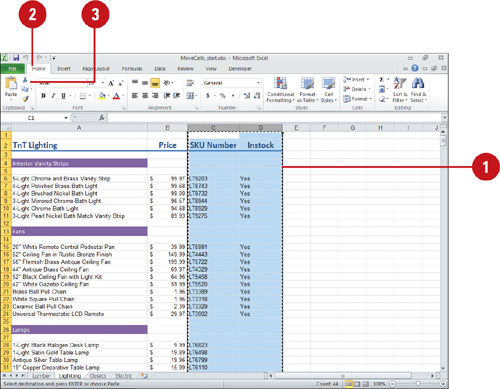
![]() Select the cells that you want to switch.
Select the cells that you want to switch.
![]() Click the Home tab.
Click the Home tab.
![]() Click the Copy button.
Click the Copy button.
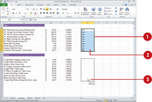
![]() Click the top-left cell of where you want to paste the data.
Click the top-left cell of where you want to paste the data.
![]() Click the Paste button arrow, point to the Transpose iconto display a live preview (New!) of the paste, and then click the Transpose icon.
Click the Paste button arrow, point to the Transpose iconto display a live preview (New!) of the paste, and then click the Transpose icon.
![]() If you want to change the way the data pastes into the document, click the Paste Options button, point to an option for the live preview (New!), andthen select the option you want.
If you want to change the way the data pastes into the document, click the Paste Options button, point to an option for the live preview (New!), andthen select the option you want.

Inserting and Deleting Cell Contents
You can insert new, blank cells anywhere on the worksheet in order to enter new data or data you forgot to enter earlier. Inserting cells moves the remaining cells in the column or row in the direction of your choice, and Excel adjusts any formulas so they refer to the correct cells. You can also delete cells if you find you don’t need them; deleting cells shifts the remaining cells to the left or up—just the opposite of inserting cells. When you delete a cell, Excel removes the actual cell from the worksheet.
Insert a Cell
![]() Select the cell or cells where you want to insert the new cell(s).
Select the cell or cells where you want to insert the new cell(s).
![]() Click the Home tab.
Click the Home tab.
![]() Click the insert Cells button arrow, and then click Insert Cells.
Click the insert Cells button arrow, and then click Insert Cells.
TIMESAVER Click the Insert Cells button to quickly insert cells to the right.
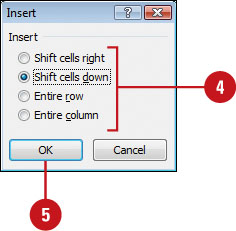
![]() Click the option you want.
Click the option you want.
![]() Shift Cells Right to move cells to the right one column.
Shift Cells Right to move cells to the right one column.
![]() Shift Cells Down to move cells down one row.
Shift Cells Down to move cells down one row.
![]() Entire Row to move the entire row down one row.
Entire Row to move the entire row down one row.
![]() Entire Column to move entire column over one column.
Entire Column to move entire column over one column.
![]() Click OK.
Click OK.

Delete a Cell
![]() Select the cell or range you want to delete.
Select the cell or range you want to delete.
![]() Click the Home tab.
Click the Home tab.
![]() Click the Delete Cells button arrow, and then click Delete Cells.
Click the Delete Cells button arrow, and then click Delete Cells.
TIMESAVER Click the Delete Cells button to quickly delete cells to the left.
![]() Click the option you want.
Click the option you want.
![]() Shift Cells Left to move the remaining cells to the left.
Shift Cells Left to move the remaining cells to the left.
![]() Shift Cells Up to move the remaining cells up.
Shift Cells Up to move the remaining cells up.
![]() Entire Row to delete the entire row.
Entire Row to delete the entire row.
![]() Entire Column to delete the entire column.
Entire Column to delete the entire column.
![]() Click OK.
Click OK.


Finding and Replacing Cell Contents
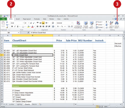
The Find and Replace commands make it easy to locate or replace specific text or formulas in a document. For example, you might want to find each figure reference in a long report to verify that the proper graphic appears. Or you might want to replace all references to cell A3 in your Excel formulas with cell G3. The Find and Replace dialog boxes vary slightly from one Office program to the next, but the commands work essentially in the same way.
Find Cell Contents
![]() Click at the beginning of the worksheet.
Click at the beginning of the worksheet.
![]() Click the Home tab.
Click the Home tab.
![]() Click the Find & Select button, and then click Find.
Click the Find & Select button, and then click Find.
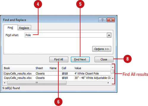
![]() Type the text you want to find.
Type the text you want to find.
![]() Click Find Next until the text you want to locate is highlighted.
Click Find Next until the text you want to locate is highlighted.
You can click Find Next repeatedly to locate each instance of the cell content.
![]() To find all cells with the contents you want, click Find All.
To find all cells with the contents you want, click Find All.
![]() If a message box opens when you reach the end of the worksheet, click OK.
If a message box opens when you reach the end of the worksheet, click OK.
![]() Click Close.
Click Close.

Replace Cell Contents
![]() Click at the beginning of the worksheet.
Click at the beginning of the worksheet.
![]() Click the Home tab.
Click the Home tab.
![]() Click the Find & Select button, and then click Replace.
Click the Find & Select button, and then click Replace.
![]() Type the text you want to search for.
Type the text you want to search for.
![]() Type the text you want to substitute.
Type the text you want to substitute.
![]() Click Find Next to begin the search, and then select the next instance of the search text.
Click Find Next to begin the search, and then select the next instance of the search text.
![]() Click Replace tosubstitute the replacement text, or click Replace All to substitute text through out the entire worksheet.
Click Replace tosubstitute the replacement text, or click Replace All to substitute text through out the entire worksheet.
You can click Find Next to locate the next instance of the cell content without making a replacement.
![]() If a message box appears when you reach the end of the worksheet, click OK.
If a message box appears when you reach the end of the worksheet, click OK.
![]() Click Close.
Click Close.

Correcting Cell Contents with AutoCorrect
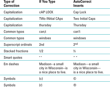
Excel’s AutoCorrect feature automatically corrects common capitalization and spelling errors as you type. AutoCorrect comes with hundreds of text and symbol entries you can edit or remove. You can add words and phrases to the AutoCorrect dictionary that you misspell, or add often-typed words and save time by just typing their initials. You could use AutoCorrect to automatically change the initials EPA to Environmental Protection Agency, for example. You can also use AutoCorrect to quickly insert symbols. For example, you can type (c) to insert ©. Use the AutoCorrect Exceptions dialog box to control how Excel handles capital letters. If you use math symbols in your work, you can use Math AutoCorrect (New!) to make it easier to insert them. It works just like AutoCorrect. When you point to a word that AutoCorrect changed, a small blue box appears under the first letter. When you point to the small blue box, the AutoCorrect Options button appears, which gives you control over whether you want the text to be corrected.
Turn On AutoCorrect
![]() Click the File tab, and then click Options.
Click the File tab, and then click Options.
![]() Click Proofing, and then click AutoCorrect Options.
Click Proofing, and then click AutoCorrect Options.
![]() Click the AutoCorrect tab.
Click the AutoCorrect tab.
![]() Select the Show AutoCorrect Options buttons check box to display the button to change AutoCorrect options when corrections arise.
Select the Show AutoCorrect Options buttons check box to display the button to change AutoCorrect options when corrections arise.
![]() Select the Replace Text As You Type check box.
Select the Replace Text As You Type check box.
![]() Select the capitalization related check boxes you want AutoCorrect to change for you.
Select the capitalization related check boxes you want AutoCorrect to change for you.
![]() To change AutoCorrect exceptions, click Exceptions, click the First Letter or INitial CAps tab, make the changes you want, and then click OK.
To change AutoCorrect exceptions, click Exceptions, click the First Letter or INitial CAps tab, make the changes you want, and then click OK.
![]() To use Math AutoCorrect (New!), click the Math AutoCorrect tab, and then select the Use Math AutoCorrect rules outside of math regions check box.
To use Math AutoCorrect (New!), click the Math AutoCorrect tab, and then select the Use Math AutoCorrect rules outside of math regions check box.
![]() Click OK, and then click OK again.
Click OK, and then click OK again.

Add or Edit an AutoCorrect Entry
![]() Click the File tab, and then click Options.
Click the File tab, and then click Options.
![]() Click Proofing, and then click AutoCorrect Options.
Click Proofing, and then click AutoCorrect Options.
![]() Click the AutoCorrect tab.
Click the AutoCorrect tab.
![]() Do one of the following:
Do one of the following:
![]() Add. Type a misspelled word or an abbreviation.
Add. Type a misspelled word or an abbreviation.
![]() Edit. Select the one you want to change. You can either type the first few letters of the entry to be changed in the Replace box, or scroll to the entry, and then click to select it.
Edit. Select the one you want to change. You can either type the first few letters of the entry to be changed in the Replace box, or scroll to the entry, and then click to select it.
![]() Type the replacement entry.
Type the replacement entry.
![]() Click Add or Replace. If necessary, click Yes to redefine entry.
Click Add or Replace. If necessary, click Yes to redefine entry.
![]() Click OK, and then click OK again.
Click OK, and then click OK again.

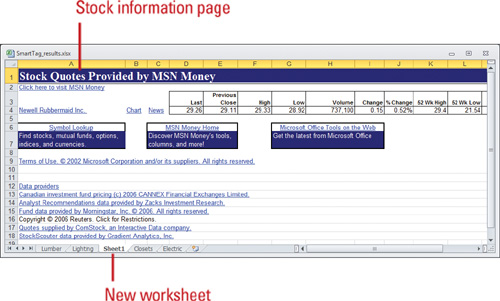
Inserting information the Smart Way
Actions (New!), a replacement for smart tags, help you integrate actions typically performed in other programs directly in Excel. For example, you can insert a financial symbol to get a stock quote, add a person’s name and address in a document to the contacts list in Microsoft Outlook, or copy and paste information with added control. Excel analyzes what you type and recognizes certain types that it marks with actions. The types of actions you can take depend on the type of data in the cell with the action. To use an action, you right-click an item to view any custom actions associated with it.
Change Options for Actions
![]() Click the File tab, and then click Options.
Click the File tab, and then click Options.
![]() In the left pane, click Proofing, and then click AutoCorrect Options.
In the left pane, click Proofing, and then click AutoCorrect Options.
![]() Click the Actions tab.
Click the Actions tab.
![]() Select the Enable additional actions in the right-click menu check box.
Select the Enable additional actions in the right-click menu check box.
![]() Select the check boxes with the actions you want.
Select the check boxes with the actions you want.
![]() To add more actions, click More Actions, and then follow the online instructions.
To add more actions, click More Actions, and then follow the online instructions.
![]() Click OK.
Click OK.
![]() Click OK again.
Click OK again.

Insert Information Using an Action
![]() Click an item, such as a cell, where you want to insert an action.
Click an item, such as a cell, where you want to insert an action.
![]() Type the information needed for the action, such as the date, a recognized financial symbol in capital letters, or a person’s name from you contacts list, and then press Spacebar.
Type the information needed for the action, such as the date, a recognized financial symbol in capital letters, or a person’s name from you contacts list, and then press Spacebar.
![]() Right-click the item, and then point to Additional Options (name varies depending on item).
Right-click the item, and then point to Additional Options (name varies depending on item).
![]() Click the action option you want; options vary depending on the action. For example, click Insert Refreshable Stock Price to insert a stock quote.
Click the action option you want; options vary depending on the action. For example, click Insert Refreshable Stock Price to insert a stock quote.
![]() In Excel, click the On a new sheet option or the Starting at cell option, and then click OK.
In Excel, click the On a new sheet option or the Starting at cell option, and then click OK.


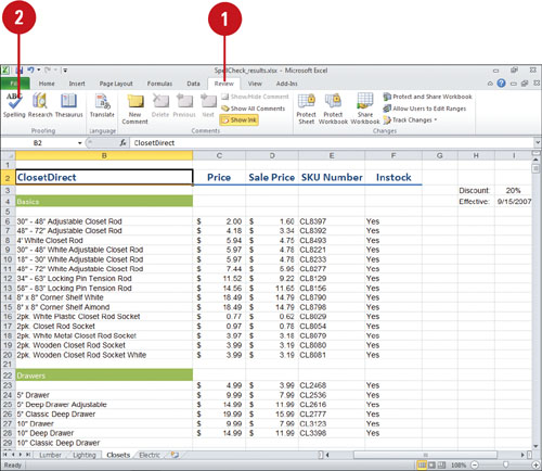
Checking Spelling
A worksheet’s textual inaccuracies can distract the reader, so it’s important that your text be error-free. Excel provides a spelling checker—common for all Office programs—so that you can check the spelling in an entire worksheet for words not listed in Excel’s dictionary (such as misspellings, names, technical terms, or acronyms) or duplicate words (such as the the). You can correct these errors as they arise or after you finish the entire workbook. You can use the Spelling button on the Review tab to check the entire workbook using the Spelling dialog box, or you can avoid spelling errors on a worksheet by enabling the AutoCorrect feature to automatically correct words as you type.
Check Spelling All at Once
![]() Click the Review tab.
Click the Review tab.
![]() Click the Spelling button.
Click the Spelling button.
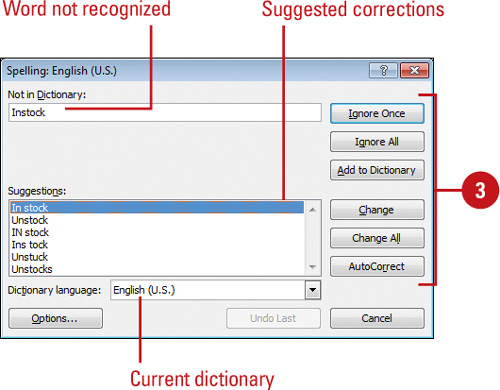
![]() If the Spelling dialog box opens, choose an option:
If the Spelling dialog box opens, choose an option:
![]() Click Ignore Once to skip the word, or click Ignore All to skip every instance of the word.
Click Ignore Once to skip the word, or click Ignore All to skip every instance of the word.
![]() Click Add to Dictionary to add a word to your dictionary, so it doesn’t show up as a misspelled word in the future.
Click Add to Dictionary to add a word to your dictionary, so it doesn’t show up as a misspelled word in the future.
![]() Click a suggestion, and then click Change or Change All.
Click a suggestion, and then click Change or Change All.
![]() Select the correct word, and then click AutoCorrect to add it to the AutoCorrect list.
Select the correct word, and then click AutoCorrect to add it to the AutoCorrect list.
![]() If no suggestion is appropriate, click in the workbook and edit the text yourself. Click Resume to continue.
If no suggestion is appropriate, click in the workbook and edit the text yourself. Click Resume to continue.
![]() Excel will prompt you when the spelling check is complete, or you can click Close to end the spelling check.
Excel will prompt you when the spelling check is complete, or you can click Close to end the spelling check.
Changing Proofing Option
You can customize the way Excel and Microsoft Office spell checks a workbook by selecting proofing settings in Excel Options. Some spelling options apply to Excel, such as Check spelling as you type, while other options apply to all Microsoft Office programs, such as Ignore Internet and file addresses, and Flag repeated words. If you have ever mistakenly used their instead of there, you can use contextual spelling to fix it. While you work in a workbook, you can can set options to have the spelling checker search for mistakes in the background.
Change Spelling Options for All Microsoft Programs
![]() Click the File tab, and then click Excel Options.
Click the File tab, and then click Excel Options.
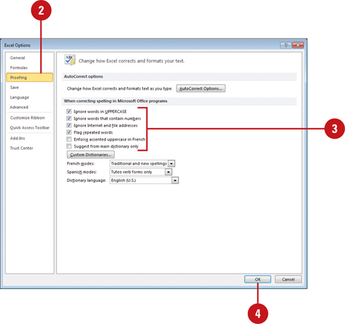
![]() In the left pane, click Proofing.
In the left pane, click Proofing.
![]() Select or clear the Microsoft Office spelling options you want.
Select or clear the Microsoft Office spelling options you want.
![]() Ignore words in UPPERCASE.
Ignore words in UPPERCASE.
![]() Ignore words that contain numbers.
Ignore words that contain numbers.
![]() Ignore Internet and file addresses.
Ignore Internet and file addresses.
![]() Flag repeated words.
Flag repeated words.
![]() Enforce accented uppercase in French.
Enforce accented uppercase in French.
![]() Suggest from main dictionary only. Selectto exclude your custom dictionary.
Suggest from main dictionary only. Selectto exclude your custom dictionary.
![]() Click OK.
Click OK.
Using Custom Dictionaries
Before you can use a custom dictionary, you need to enable it first. You can enable and manage custom dictionaries by using the Custom Dictionaries dialog box. In the dialog box, you can change the language associated with a custom dictionary, create a new custom dictionary, or add or remove existing custom dictionary. If you need to manage dictionary content, you can also change the default custom dictionary to which the spelling checker adds words, as well as add, delete, or edit words. All the modifications you make to your custom dictionaries are shared with all your Microsoft Office programs, so you only need to make changes once. If you mistakenly type an obscene or embarrassing word, such as ass instead of ask, the spelling checker will not catch it because both words are spelled correctly. You can avoid this problem by using an exclusion dictionary. When you use a language for the first time, Office automatically creates an exclusion dictionary. This dictionary forces the spelling checker to flag words you don’t want to use.
Use a Custom Dictionary
![]() Click the File tab, and then click Options.
Click the File tab, and then click Options.
![]() In the left pane, click Proofing.
In the left pane, click Proofing.
![]() Click Custom Dictionaries.
Click Custom Dictionaries.
![]() Select the check box next to CUSTOM.DIC (Default).
Select the check box next to CUSTOM.DIC (Default).
![]() Click the Dictionary language list arrow, and then select a language for a dictionary.
Click the Dictionary language list arrow, and then select a language for a dictionary.
![]() Click the options you want:
Click the options you want:
![]() Click Edit Word List toadd, delete, or edit words.
Click Edit Word List toadd, delete, or edit words.
![]() Click Change Default to select a new default dictionary.
Click Change Default to select a new default dictionary.
![]() Click New to create a new dictionary.
Click New to create a new dictionary.
![]() Click Add to insert an existing dictionary.
Click Add to insert an existing dictionary.
![]() Click Remove to delete a dictionary.
Click Remove to delete a dictionary.
![]() Click OK to close the Custom Dictionaries dialog box.
Click OK to close the Custom Dictionaries dialog box.
![]() Click OK.
Click OK.

Find and Modify the Exclusion Dictionary
![]() In Windows Explorer, go to the folder location where the custom dictionaries are stored.
In Windows Explorer, go to the folder location where the custom dictionaries are stored.
![]() Windows 7 or Vista. C:Usersuser nameAppDataRoamingMicrosoftUProof
Windows 7 or Vista. C:Usersuser nameAppDataRoamingMicrosoftUProof
![]() Windows XP. C:Documents and Settings user nameApplication DataMicrosoftUProof
Windows XP. C:Documents and Settings user nameApplication DataMicrosoftUProof
TROUBLE? If you can’t find the folder, change folder settings to show hidden files and folders.
![]() Locate the exclusion dictionary for the language you want to change.
Locate the exclusion dictionary for the language you want to change.
![]() The file name you want is ExcludeDictionary Language CodeLanguage LCID. lex.
The file name you want is ExcludeDictionary Language CodeLanguage LCID. lex.
For example, ExcludeDictionary EN0409.lex, where EN is for English.
Check Excel Help for an updated list of LCID (Local Identification Number) number for each language.
![]() Open the file using Microsoft Notepad or WordPad.
Open the file using Microsoft Notepad or WordPad.
![]() Add each word you want the spelling check to flag as misspelled. Type the words in all lowercase and then press Enter after each word.
Add each word you want the spelling check to flag as misspelled. Type the words in all lowercase and then press Enter after each word.
![]() Save and close the file.
Save and close the file.

Inserting Symbols
Excel comes with a host of symbols for every need. Insert just the right one to keep from compromising a workbook’s professional appearance with a missing accent or mathematical symbol (å). In the Symbol dialog box, you use the Recently used symbols list to quickly insert a symbol that you want to insert again. If you don’t see the symbol you want, use the Font list to look at the available symbols for other fonts installed on your computer.
Insert Symbols and Special Characters
![]() Click the document where you want to insert a symbol or character.
Click the document where you want to insert a symbol or character.
![]() Click the Insert tab, and then click the Symbol button.
Click the Insert tab, and then click the Symbol button.
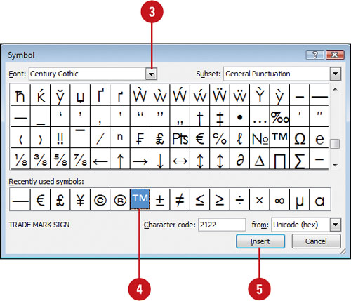
![]() To see other symbols, click the Font list arrow, and then click a new font.
To see other symbols, click the Font list arrow, and then click a new font.
![]() Click a symbol or character.
Click a symbol or character.
You can use the Recently used symbols list to use a symbol you’ve already used.
![]() Click insert.
Click insert.
Finding the Right Words
Repeating the same word in a workbook can reduce a message’s effectiveness. Instead, replace some words with synonyms or find antonyms. If you need help finding exactly the right words, use the shortcut menu to look up synonyms quickly or search a Thesaurus for more options. This feature can save you time and improve the quality and readability of your workbook. You can also install a Thesaurus for another language. Foreign language thesauruses can be accessed under Research Options on the Research task pane.
Use the Thesaurus
![]() Select the text you want to translate.
Select the text you want to translate.
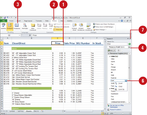
![]() Click the Review tab.
Click the Review tab.
![]() Click the Thesaurus button.
Click the Thesaurus button.
![]() Click the list arrow, and then select a Thesaurus, if necessary.
Click the list arrow, and then select a Thesaurus, if necessary.
![]() Point to the word in the Research task pane.
Point to the word in the Research task pane.
![]() Click the list arrow, and then click one of the following:
Click the list arrow, and then click one of the following:
![]() Insert to replace the word you looked up with the new word.
Insert to replace the word you looked up with the new word.
![]() Copy to copy the new word and then paste it within the workbook.
Copy to copy the new word and then paste it within the workbook.
![]() Look Up to look up the word for other options.
Look Up to look up the word for other options.
![]() When you’re done, click the Close button on the task pane.
When you’re done, click the Close button on the task pane.
Inserting Research Material
With the Research task pane, you can access data sources and insert research material right into your text without leaving your Excel workbook. The Research task pane can help you access electronic dictionaries, thesauruses, research sites, and proprietary company information. You can select one reference source or search in all reference books. This research pane allows you to find information and quickly and easily incorporate it into your work.
Research a topic
![]() Click the Review tab.
Click the Review tab.
![]() Click the Research button.
Click the Research button.
![]() Type the topic you would like to research.
Type the topic you would like to research.
![]() Click the list arrow, and then select a reference source, or click All Reference Books.
Click the list arrow, and then select a reference source, or click All Reference Books.
![]() To customize which resources are used for translation, click Research options, select the reference books and research sites you want, and then click OK.
To customize which resources are used for translation, click Research options, select the reference books and research sites you want, and then click OK.
![]() Click the Start Searching button (green arrow).
Click the Start Searching button (green arrow).
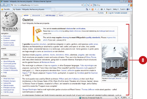
![]() Select the information in the Research task pane that you want to copy.
Select the information in the Research task pane that you want to copy.
To search for more information, click one of the words in the list or click a link to an online site, such as Wikipedia.
![]() Select the information you want, and then copy it.
Select the information you want, and then copy it.
In the Research task pane, you can point to the item you want, click the list arrow, and then click Copy.
![]() Paste the information into your workbook.
Paste the information into your workbook.
![]() When you’re done, click the Close button on the task pane.
When you’re done, click the Close button on the task pane.

Translating Text to Another Language
With the Research task pane, you can translate single words or short phrases into different languages by using bilingual dictionaries. The Research task pane provides you with different translations and allows you to incorporate it into your work. If you need to translate an entire document for basic subject matter understanding, Web-based machine translations services are available. A machine translation is helpful for general meaning, but may not preserve the full meaning of the content.
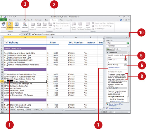
Translate Text
![]() Select the text you want to translate.
Select the text you want to translate.
![]() Click the Review tab.
Click the Review tab.
![]() Click the Translate button.
Click the Translate button.
If this is the first you have used translation services, click OK to install the bilingual dictionaries and enable the service.
![]() If necessary, click the list arrow, and then click Translation.
If necessary, click the list arrow, and then click Translation.
![]() Click the From list arrow, and then select the language of the selected text.
Click the From list arrow, and then select the language of the selected text.
![]() Click the To list arrow, and then select the language you want to translate into.
Click the To list arrow, and then select the language you want to translate into.
![]() To customize which resources are used for translation, click Translation options, select the look-up options you want, and then click OK.
To customize which resources are used for translation, click Translation options, select the look-up options you want, and then click OK.
![]() Right-click the translated text in the Research task pane that you want to copy, and then click Copy.
Right-click the translated text in the Research task pane that you want to copy, and then click Copy.
![]() Paste the information into your workbook.
Paste the information into your workbook.
![]() When you’re done, click the Close button on the task pane.
When you’re done, click the Close button on the task pane.
Undoing and Redoing an Action
You may realize you’ve made a mistake shortly after completing an action or a task. The Undo feature lets you “take back” one or more previous actions, including data you entered, edits you made, or commands you selected. For example, if you were to enter a number in a cell, and then decide the number was incorrect, you could undo the entry instead of selecting the data and deleting it. A few moments later, if you decide the number you deleted was correct after all, you could use the Redo feature to restore it to the cell.
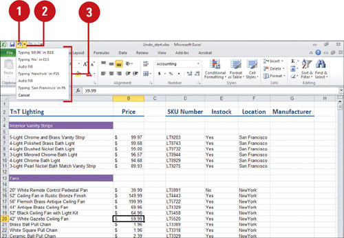
Undo an Action
![]() Click the Undo button on the Quick Access Toolbar to undo the last action you completed.
Click the Undo button on the Quick Access Toolbar to undo the last action you completed.
![]() Click the Undo button arrow on the Quick Access Toolbar to see recent actions that can be undone.
Click the Undo button arrow on the Quick Access Toolbar to see recent actions that can be undone.
![]() Click an action. Excel reverses the selected action and all actions above it.
Click an action. Excel reverses the selected action and all actions above it.
Redo an Action
![]() Click the Redo button on the Quick Access Toolbar to restore your last undone action.
Click the Redo button on the Quick Access Toolbar to restore your last undone action.
TROUBLE? If the Redo button is not available on the Quick Access Toolbar, click the Customize Quick Access Toolbar list arrow, and then click Redo.
![]() Click the Redo button arrow on the Quick Access Toolbar to see actions that can be restored.
Click the Redo button arrow on the Quick Access Toolbar to see actions that can be restored.
![]() Click the action you want to restore. All actions above it will be restored as well.
Click the action you want to restore. All actions above it will be restored as well.
