
Measurement Data Analysis
A great deal of useful information can be obtained by analyzing field measurement information, but archived information is usually only reviewed when a question is raised concerning a specific metering point. The analysis of corrected volumes can provide insight into system balance/lost and unaccounted for (LUAF) levels and direction. Analysis of the archived average differential pressure can provide a number of indicators. The average flowing temperature is archived in support of the volume determination, but its determination is far from simple. The volumetric measurement of a fluid mixture, as opposed to a pure fluid, requires analysis of the fluid in order to identify the magnitude of the various components of the mixture. Flow time in hours, days, and/or months can provide valuable information on the proper operation of the measurement station. The usefulness of these measures is discussed in this chapter.
Keywords
field measurement data; analysis; corrected volumes; average differential pressure; flowing temperature; volumetric measurement; flow time
Introduction
During the course of performing the fluid measurement function, large quantities of field measurement information is gathered, either manually or electronically, in support of the quantity determination, contractual and/or regulatory compliance, and/or operational support. This information is in the form of uncorrected volumes, corrected volumes, mass, energy, energy per unit volume, fluid analysis, average differential pressure, average static pressure, average flowing temperature, flow time, average velocity, and, if available, meter diagnostics. This information is normally stored as hard copy or in an electronic data warehouse. The review of such data, if it occurs, is usually relegated to the overburdened field measurement technician or, in the office, to an overburdened individual or one who does not have the experience to assess the information effectively. Therefore very little benefit is obtained from the archived measurement information. In fact, the archived information is usually only reviewed when a question is raised concerning a specific metering point. However, if routine analysis is performed on the archived measurement information in the form of measurement control charts, a great deal of useful information can be obtained and used to determine the measurement health of a given metering point. Even more importantly, that analysis information can be used very effectively to manage system balance/LUAF levels. The following discussion will demonstrate the type of benefit that be obtained from routine measurement information analysis.
Corrected Volume
In all cases corrected volumes are required to be archived for a substantial period of time (years). Analysis of these volumes can provide insight into system balance/LUAF levels and direction. As an example on a system that is primarily composed of differential head meters and is already showing a significant (greater than 0.6%) annual negative loss per year, a corrected volume control chart that shows corrected volume input versus corrected volume output could indicate the outcome of increasing the volume through the system. Figure 16-1 is such a chart and it indicates that increasing the volume through the system will most likely increase the loss.

Knowing that the system was composed mainly of differential head meters led one to suspect that the system was suffering a serious contamination problem in the outlet meters. Differential head meters tend to under-register when contaminated. This was borne out through site audits of the 60 controlling outlet metering stations. Once identified and corrected, the system balance/LUAF returned to acceptable levels and the system was able to increase its volume.
Differential Pressure
Analysis of the archived average differential pressure can provide a number of indicators:
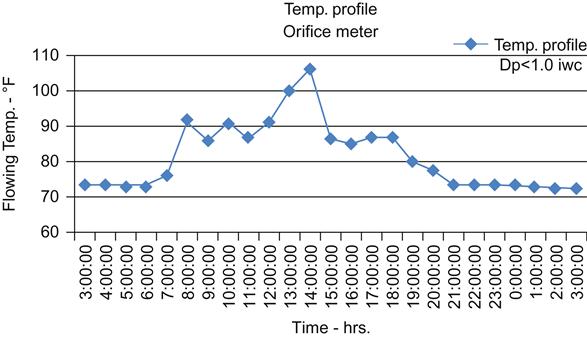
1. Meter station average low hourly or daily differential pressure—the differential head meter is most likely too large, see Figure 16-2. Best measurement practices recommend that the differential to continually operate above 10 inches of water or 10% of the upper range value of the transmitter. Occasional excursions below the recommendation are acceptable, but only for very short period of time.
Figure 16-2 was developed while flow-calibrating the coefficient of discharge, Cd, for an orifice plate using a smart differential pressure, Dp, transmitter which was statically calibrated to less than 1 inch of water column, iwc. During this calibration the Dp was selectively reduced to less than 1 iwc. In doing this the Cd data points show increasing data scatter until at less than 1 iwc the scatter is in excess of 5%. A flow computer sampling at the low Dp would incur a greater flow uncertainty of in excess of ±2.5%.
2. System-wide seasonal low differential pressures—on a system that is composed predominately of differential head meters, see Figures 16-3 and 16-4, this indicates seasonal system load fluctuations.
From the pipeline system balance/LUAF shown in Figures 16-3 and 16-4, it can be seen that there appears to be an established seasonal relationship. This seasonal relationship shows that the system balance/LUAF is less in the winter but greater in the summer. This appears to be a load (throughput) relationship. Looking at the number of low monthly Dp receipt and delivery meters shows that the receipts do not emulate the seasonal system balance/LUAF relationship (Figures 16-5 to 16-8).
However, the number of low monthly Dp delivery meters do emulate the seasonal system balance/LUAF relationship. The larger the number of low Dp meters, the greater the system imbalance/LUAF percentage loss. Therefore, the issue is within the delivery volumes. Pipeline personnel tend to install the largest orifice bore diameter that their measurement procedures will allow in order to avoid being called out to change plates when deliveries increase, which results in low Dp during low delivery periods. This is a low Dp (less than 10 iwc) issue. Thus changing the orifice plate bore size to maintain higher Dp during low delivery summer months will improve the system balance/LUAF.


Flowing Temperature
Determination of the flowing temperature would appear to be a rather straightforward operation. A temperature measurement device is installed in the pipe in a temperature well (thermowell) in which a conducting fluid has been placed. The thermowell is used in order to isolate the temperature transmitter from the pipeline operating pressure. The output of the temperature transmitter is monitored and data from it is collected for onsite or remote determination of flow. The average flowing temperature is archived in support of the volume determination. This is a very simple concept on the surface, but it does have its complexities. In the process of performing the temperature measurement function, the temperature transmitter is exposed to the ambient environment of the pipeline, in particular the ambient temperature, resulting in conduction, convection, and radiant heat transfer with the ambient acting as an infinite source or sink. This ambient heat transfer tends to influence the thermowell and the pipe to which it is attached. This influence usually results in a biased temperature measurement which is a function of the ambient temperature. If the fluid entering the metering station is cooler than the ambient environment, then the resulting temperature measurement bias would be an over-registration of temperature. However, if the fluid temperature is warmer than the ambient environment, then the resulting temperature measurement bias would be an under-registration of temperature. In gas measurement, the measured temperature bias would be 0.1% per degree for differential head meters and 0.2% per degree for linear meters.
This issue is amplified by the size of the pipe and the velocity of the entering gas; the lower the gas velocity and the smaller the pipe, the greater the bias. In addition, covering the meter run or station will only mitigate the radiant component of the influence. Figures 16-9 and 16-10 demonstrate this influence on a differential head meter and a linear meter.

Figures 16-9 and 16-10 are for the same meter with the same ambient temperature environment but with different differential pressures and gas velocities. The gas temperature entering the meter run/station was 60°F in both cases. The influence of ambient temperature, as one might suspect, does not appear to be linear (Figures 16-11 and 16-12).


These data show that this influence is not a meter issue but rather a piping and velocity issue. It becomes a measurement issue when the “measured temperature” is used in the calculation of corrected volume. If all the meters in a system were of the same type, differential or linear, and all experienced the same ambient temperature environment, then the influence would not significantly impact the system balance. However, this is not normally the case.
The liquid segment of the energy industry appears to be more conscious of this phenomenon, since it is common practice to insulate from the meter downstream through the temperature measurement thus mitigating this influence.
Fluid Analysis
The volumetric measurement of a fluid mixture, as opposed to a pure fluid, requires analysis of the fluid in order to identify the magnitude of the various components of the mixture. Knowledge of the components of the mixture is essential for volumetric measurement. One might attempt to avoid the need to analyze by utilizing direct (as opposed to inferred) mass measurement. However, this results in knowing the mass of a mixture which is usually not adequate. In natural gas volumetric and energy measurement, the compositional analysis is used to determine the energy per unit volume and the relative density (specific gravity). Maintaining control charts on the analyzed properties can provide warnings of incorrect values; see Figure 16-13.

Flow Time
Flow time in hours, days, and/or months can provide valuable information on the proper operation of the measurement station. Successful completion of the designated flow time period assures the practitioner that the measurement has remained within the acceptable range of the meter, thus allowing the practitioner to assess and/or manage the overall measurement uncertainty. Figure 16-14 shows a metering installation where the flow time consistently fails to complete the time interval, hour. This may be an indication of an oversized meter, in the case of a linear meter, or the need to adjust the bore size of a differential head meter, i.e., an orifice meter. It can also indicate that the metering range is so large that an additional meter or a different type of meter is required.

Consistently failing to complete the time period usually results in under-registration of flow.