
Simulations and Reductions
Abstract
In complexity theory, it is common to prove results by reduction from one problem to another. For example, textbooks typically prove from first principles that satisfiability (SAT) is NP complete. To show that another problem is also NP-complete, it is enough to show that SAT (or some other problem known to be NP-complete) reduces to the problem in question. Reductions are appealing because they are often technically simpler than proving NP completeness directly.
Reductions can also be applied in distributed computing. This chapter describes a general technique for showing that a protocol in one model can be transformed into a protocol in another model. In addition, we describe a specific transformation, called BG simulation.
Keywords
BG simulation; Reduction; Simulation
We present here a general combinatorial framework to translate impossibility results from one model of computation to another. Once one has proved an impossibility result in one model, one can avoid reproving that result in related models by relying on reductions. The combinatorial framework explains how the topology of the protocol complexes in the two models have to be related to be able to obtain a reduction. We also describe an operational framework consisting of an explicit distributed simulation protocol that implements reductions. Although this protocol provides algorithmic intuition behind the combinatorial simulation framework and may even be of practical interest, a key insight behind this chapter is that there is often no need to construct such explicit simulations. Instead, we can treat simulation as a task like any other and apply the computability conditions of Chapter 5 to show when a simulation protocol exists. These existence conditions are given in terms of the topological properties of the models’ protocol complexes instead of devising pair-wise simulations.
7.1 Motivation
Modern distributed systems are highly complex yet reliable and efficient, thanks to heavy use of abstraction layers in their construction. At the hardware level processes may communicate through low-level shared-register operations, but a programmer uses complex shared objects to manage concurrent threads. Also from the theoretical perspective, researchers have devised algorithms to implement higher-level-of-abstraction shared objects from lower-level-of-abstraction objects. We have already encountered this technique to build larger set agreement boxes from smaller ones (Exercise 5.6) or to implement snapshots from single-writer/multireader registers (Exercise 4.12). We say snapshots can be simulated in a wait-free system where processes communicate using single-writer/single-reader registers. Simulations are useful also to deduce the relative power of abstractions; in this case, snapshots are as powerful as single-writer/single-reader registers, but not more powerful. In contrast, a consensus shared black box cannot be simulated in a wait-free system where processes communicate using only read-write registers, as we have already seen.
Software systems are built in a modular fashion using this simulation technique, assuming a black box for a problem has been constructed and using it to further extend the system. However, this technique is also useful to prove impossibility results. In complexity theory, it is common to prove results by reduction from one problem to another. For example, to prove that there is not likely to exist a polynomial algorithm for a problem, one may try to show that the problem is NP-complete. Textbooks typically prove from first principles that satisfiability (SAT) is NP-complete. To show that another problem is also NP-complete, it is enough to show that SAT (or some other problem known to be NP-complete) reduces to the problem in question. Reductions are appealing because they are often technically simpler than proving NP completeness directly.
Reductions can also be applied in distributed computing for impossibility results. For example, suppose we know that a colorless task has no wait-free layered immediate snapshot protocol, and we want to know whether it has a ![]() -resilient protocol for some
-resilient protocol for some ![]() . One way to answer this question is to assume that an
. One way to answer this question is to assume that an ![]() -process,
-process, ![]() -resilient protocol exists and devise a wait-free protocol where
-resilient protocol exists and devise a wait-free protocol where ![]() processes “simulate” the
processes “simulate” the ![]() -resilient
-resilient ![]() -process protocol execution in the following sense: The
-process protocol execution in the following sense: The ![]() -processes use the code for the protocol to simulate an execution of the
-processes use the code for the protocol to simulate an execution of the ![]() -processes. They assemble mutually consistent final views of an
-processes. They assemble mutually consistent final views of an ![]() -process protocol execution during which at most
-process protocol execution during which at most ![]() processes may fail. Each process halts after choosing the output value that would have been chosen by one of the simulated processes. Because the task is colorless, any process can choose any simulated process’s output, so this simulation yields a wait-free
processes may fail. Each process halts after choosing the output value that would have been chosen by one of the simulated processes. Because the task is colorless, any process can choose any simulated process’s output, so this simulation yields a wait-free ![]() -process layered protocol, contradicting the hypothesis that no such protocol exists. Instead of proving directly that no
-process layered protocol, contradicting the hypothesis that no such protocol exists. Instead of proving directly that no ![]() -resilient protocol exists, we reduce the
-resilient protocol exists, we reduce the ![]() -resilient problem to the previously solved wait-free problem.
-resilient problem to the previously solved wait-free problem.
In general, we can use simulations and reductions to translate impossibility results from one model of computation to another. As in complexity theory, once one has proved an impossibility result in one model, one can avoid reproving that result in related models by relying on reductions. One possible problem with this approach is that known simulation techniques, such as the BG-simulation protocol presented in Section 7.4, are model-specific, and a new, specialized simulation protocol must be crafted for each pair of models. Moreover, given two models, how do we know if there is a simulation before we start to try to design one?
The key insight behind this chapter is that there is often no need to construct explicit simulations. Instead, we can treat simulation as a task like any other and apply the computability conditions of Chapter 5 to show when a simulation protocol exists. These existence conditions are given in terms of the topological properties of the models’ protocol complexes and are likely to be easier to determine in general than devising pair-wise simulations. Once it is known that a simulation exists, one may then concentrate on finding an efficient one that might be of practical interest.
7.2 Combinatorial setting
So far we have considered several models of computation. Each one is given by a set of process names, ![]() ; a communication medium, such as shared memory or message-passing; a timing model, such as synchronous or asynchronous; and a failure model, given by an adversary,
; a communication medium, such as shared memory or message-passing; a timing model, such as synchronous or asynchronous; and a failure model, given by an adversary, ![]() . For each model of computation, once we fix a colorless input complex
. For each model of computation, once we fix a colorless input complex ![]() , we may consider the set of final views of a protocol. We have the combinatorial definition of a protocol (Definition 4.2.2), as a triple
, we may consider the set of final views of a protocol. We have the combinatorial definition of a protocol (Definition 4.2.2), as a triple ![]() where
where ![]() is an input complex,
is an input complex, ![]() is a protocol complex (of final views), and
is a protocol complex (of final views), and ![]() is an execution map. For each
is an execution map. For each ![]() , a model of computation may be represented by all the protocols on
, a model of computation may be represented by all the protocols on ![]() .
.
Definition 7.2.1
A model of computation ![]() on an input complex
on an input complex ![]() is a (countably infinite) family of protocols
is a (countably infinite) family of protocols ![]() .
.
Consider for instance the ![]() -process, colorless layered immediate snapshot protocol of Chapter 4. If we take the wait-free adversary and any input complex
-process, colorless layered immediate snapshot protocol of Chapter 4. If we take the wait-free adversary and any input complex ![]() , the model
, the model ![]() obtained consists of all protocols
obtained consists of all protocols ![]() , corresponding to having the layered immediate snapshot protocol execute
, corresponding to having the layered immediate snapshot protocol execute ![]() layers, where
layers, where ![]() is the complex of final configurations and
is the complex of final configurations and ![]() the corresponding carrier map. Similarly, taking the
the corresponding carrier map. Similarly, taking the ![]() -resilient layered immediate snapshot protocol of Figure 5.1 for
-resilient layered immediate snapshot protocol of Figure 5.1 for ![]() processes and input complex
processes and input complex ![]() consists of all protocols
consists of all protocols ![]() , corresponding to executing the protocol for
, corresponding to executing the protocol for ![]() layers.
layers.
Definition 7.2.2
A model of computation ![]() solves a colorless task
solves a colorless task ![]() if there is a protocol in
if there is a protocol in ![]() that solves that task.
that solves that task.
Recall that a protocol ![]() solves a colorless task
solves a colorless task ![]() if there is a simplicial map
if there is a simplicial map ![]() carried by
carried by ![]() . Operationally, in each execution, processes end up with final views that are vertices of the same simplex
. Operationally, in each execution, processes end up with final views that are vertices of the same simplex ![]() of
of ![]() . Moreover, if the input simplex of the execution is
. Moreover, if the input simplex of the execution is ![]() , then
, then ![]() . Each process finishes the protocol in a local state that is a vertex of
. Each process finishes the protocol in a local state that is a vertex of ![]() and then applies
and then applies ![]() to choose an output value. These output values form a simplex in
to choose an output value. These output values form a simplex in ![]() .
.
For example, the model ![]() solves the iterated barycentric agreement task
solves the iterated barycentric agreement task ![]() for any
for any ![]() . To see this, we must verify that there is some
. To see this, we must verify that there is some ![]() such that the protocol
such that the protocol ![]() solves
solves ![]() .
.
A reduction is defined in terms of two models of computation: a model ![]() (called the real model) and a model
(called the real model) and a model ![]() (called the virtual model). They have the same input complex
(called the virtual model). They have the same input complex ![]() , but their process names, protocol complexes, and adversaries may differ. The real model reduces to the virtual model if the existence of a protocol in the virtual model implies the existence of a protocol in the real model.
, but their process names, protocol complexes, and adversaries may differ. The real model reduces to the virtual model if the existence of a protocol in the virtual model implies the existence of a protocol in the real model.
For example, the ![]() -resilient layered immediate snapshot model
-resilient layered immediate snapshot model ![]() for
for ![]() processes trivially reduces to the wait-free model
processes trivially reduces to the wait-free model ![]() . Operationally it is clear why. If a wait-free
. Operationally it is clear why. If a wait-free ![]() -process protocol solves a task
-process protocol solves a task ![]() it tolerates failures by
it tolerates failures by ![]() processes. The same protocol solves the task if only
processes. The same protocol solves the task if only ![]() out of the
out of the ![]() may crash. Combinatorially, the definition of reduction is as follows.
may crash. Combinatorially, the definition of reduction is as follows.
Definition 7.2.3
Let ![]() be an input complex and
be an input complex and ![]() be two models on
be two models on ![]() . The (real) model
. The (real) model ![]() reduces to the (virtual) model
reduces to the (virtual) model ![]() if, for any colorless task
if, for any colorless task ![]() with input complex
with input complex ![]() , a protocol for
, a protocol for ![]() in
in ![]() implies that there is a protocol for
implies that there is a protocol for ![]() in
in ![]() .
.
We typically demonstrate reduction using simulation.
Definition 7.2.4
Let ![]() be a protocol in
be a protocol in ![]() and
and ![]() a protocol in
a protocol in ![]() . A simulation is a simplicial map
. A simulation is a simplicial map
![]()
such that for each simplex ![]() in
in ![]() maps
maps ![]() to
to ![]() .
.
The operational intuition is that each process executing the real protocol chooses a simulated execution in the virtual protocol, where each virtual process has the same input as some real process. However, from a combinatorial perspective, it is sufficient to show that there exists a simplicial map ![]() as above. Note that
as above. Note that ![]() may be collapsing: Real processes with distinct views may choose the same view of the simulated execution.
may be collapsing: Real processes with distinct views may choose the same view of the simulated execution.
The left-hand diagram of Figure 7.1 illustrates how a protocol solves a task. Along the horizontal arrow, ![]() carries each input simplex
carries each input simplex ![]() of
of ![]() to a subcomplex of
to a subcomplex of ![]() . Along the diagonal arrow, a protocol execution, here denoted
. Along the diagonal arrow, a protocol execution, here denoted ![]() , carries each
, carries each ![]() to a subcomplex of its protocol complex, denoted by
to a subcomplex of its protocol complex, denoted by ![]() , which is mapped to a subcomplex of
, which is mapped to a subcomplex of ![]() along the vertical arrow by the simplicial map
along the vertical arrow by the simplicial map ![]() . The diagram semi-commutes: The subcomplex of
. The diagram semi-commutes: The subcomplex of ![]() reached through the diagonal and vertical arrows is contained in the subcomplex reached through the horizontal arrow.
reached through the diagonal and vertical arrows is contained in the subcomplex reached through the horizontal arrow.

Figure 7.1 Carrier maps are shown as dashed arrows, simplicial maps as solid arrows. On the left, ![]() via
via ![]() solves the colorless task
solves the colorless task ![]() . In the middle,
. In the middle, ![]() simulates
simulates ![]() via
via ![]() . On the right,
. On the right, ![]() via the composition of
via the composition of ![]() and
and ![]() solves
solves ![]() .
.
Simulation is illustrated in the middle diagram of Figure 7.1. Along the diagonal arrow, ![]() carries each input simplex
carries each input simplex ![]() of
of ![]() to a subcomplex of its protocol complex
to a subcomplex of its protocol complex ![]() . Along the vertical arrow,
. Along the vertical arrow, ![]() carries each input simplex
carries each input simplex ![]() of
of ![]() to a subcomplex of its own protocol complex
to a subcomplex of its own protocol complex ![]() , which is carried to a subcomplex of
, which is carried to a subcomplex of ![]() by the simplicial map
by the simplicial map ![]() . The diagram semi-commutes: The subcomplex of
. The diagram semi-commutes: The subcomplex of ![]() reached through the vertical and horizontal arrows is contained in the subcomplex reached through the diagonal arrow. Thus, we may view simulation as solving a task. If we consider
reached through the vertical and horizontal arrows is contained in the subcomplex reached through the diagonal arrow. Thus, we may view simulation as solving a task. If we consider ![]() as a task, where
as a task, where ![]() is input complex and
is input complex and ![]() is output complex, then
is output complex, then ![]() solves this task with decision map
solves this task with decision map ![]() carried by
carried by ![]() .
.
Theorem 7.2.5
If every protocol in ![]() can be simulated by a protocol in
can be simulated by a protocol in ![]() , then
, then ![]() reduces to
reduces to ![]() .
.
Proof
Recall that if ![]() has a protocol
has a protocol ![]() for a colorless task
for a colorless task ![]() , then there is a simplicial map
, then there is a simplicial map ![]() carried by
carried by ![]() , that is,
, that is, ![]() for each
for each ![]() . If model
. If model ![]() simulates model
simulates model ![]() , then for any protocol
, then for any protocol ![]() has a protocol
has a protocol ![]() in
in ![]() and a simplicial map
and a simplicial map ![]() such that for each simplex
such that for each simplex ![]() in
in ![]() .
.
Let ![]() be the composition of
be the composition of ![]() and
and ![]() . To prove that
. To prove that ![]() solves
solves ![]() with
with ![]() , we need to show that
, we need to show that ![]() . By construction,
. By construction,
![]()
so ![]() also solves
also solves ![]() .
. ![]()
Theorem 7.2.5 depends only on the existence of a simplicial map. Our focus in the first part of this chapter is to establish conditions under which such maps exist. In the second part, we will construct one operationally.
7.3 Applications
In Chapters 5 and 6, we gave necessary and sufficient conditions for solving colorless tasks in a variety of computational models. Table 7.1 lists these models, parameterized by an integer ![]() . We proved that the colorless tasks that can be solved by these models are the same and those colorless tasks
. We proved that the colorless tasks that can be solved by these models are the same and those colorless tasks ![]() for which there is a continuous map
for which there is a continuous map
![]()
carried by ![]() . Another way of proving this result is showing that these protocols are equivalent in the simulation sense of Definition 7.2.4.
. Another way of proving this result is showing that these protocols are equivalent in the simulation sense of Definition 7.2.4.
Lemma 7.3.1
Consider any input complex ![]() and any two models
and any two models ![]() and
and ![]() with
with ![]() . For any protocol
. For any protocol ![]() in
in ![]() there is a protocol
there is a protocol ![]() in
in ![]() and a simulation map
and a simulation map
![]()
carried by ![]() .
.

Here are some of the implications of this lemma, together with Theorem 7.2.5:
• A ![]() -process wait-free model can simulate an
-process wait-free model can simulate an ![]() -process wait-free model, and vice versa. We will give an explicit algorithm for this simulation in the next section.
-process wait-free model, and vice versa. We will give an explicit algorithm for this simulation in the next section.
• If ![]() , an
, an ![]() -process
-process ![]() -resilient message-passing model can simulate an
-resilient message-passing model can simulate an ![]() -process
-process ![]() -resilient layered immediate snapshot model, and vice versa.
-resilient layered immediate snapshot model, and vice versa.
• Any adversary model can simulate any other adversary model for which the minimum core size is the same or larger. In particular, all adversaries with the same minimum core size are equivalent.
• An adversarial model with minimum core size ![]() can simulate a wait-free
can simulate a wait-free ![]() -set layered immediate snapshot model.
-set layered immediate snapshot model.
• A ![]() -resilient Byzantine model can simulate a
-resilient Byzantine model can simulate a ![]() -resilient layered immediate snapshot model if
-resilient layered immediate snapshot model if ![]() is sufficiently small:
is sufficiently small: ![]() .
.
7.4 BG simulation
In this section, we construct an explicit shared-memory protocol by which ![]() processes running against adversary
processes running against adversary ![]() can simulate
can simulate ![]() processes running against adversary
processes running against adversary ![]() , where
, where ![]() and
and ![]() have the same minimum core size. We call this protocol BG simulation after its inventors, Elizabeth Borowsky and Eli Gafni. As noted, the results of the previous section imply that this simulation exists, but the simulation itself is an interesting example of a concurrent protocol.
have the same minimum core size. We call this protocol BG simulation after its inventors, Elizabeth Borowsky and Eli Gafni. As noted, the results of the previous section imply that this simulation exists, but the simulation itself is an interesting example of a concurrent protocol.
7.4.1 Safe agreement
The heart of the BG simulation is the notion of safe agreement. Safe agreement is similar to consensus except it is not wait-free (nor is it a colorless task; see Chapter 11). Instead, there is an unsafe region during which a halting process will block agreement. This unsafe region encompasses a constant number of steps. Formally, safe agreement satisfies these conditions:
• Validity. All processes that decide will decide some process’s input.
• Agreement. All processes that decide will decide the same value.
To make it easy for processes to participate in multiple such protocols simultaneously, the safe agreement illustrated in Figure 7.2 is split into two methods: propose(v)and resolve(). When a process joins the protocol with input ![]() , it calls propose(v)once. When a process wants to discover the protocol’s result, it calls resolve(), which returns either a value or
, it calls propose(v)once. When a process wants to discover the protocol’s result, it calls resolve(), which returns either a value or ![]() if the protocol has not yet decided. A process may call resolve()multiple times.
if the protocol has not yet decided. A process may call resolve()multiple times.

The processes share two arrays: announce[]holds each process’s input, and level[]holds each process’s level, which is 0, 1, or 2. Each ![]() starts by storing its input in announce[i], making that input visible to the other processes (Line 9). Next,
starts by storing its input in announce[i], making that input visible to the other processes (Line 9). Next, ![]() raises its level from 0 to 1 (Line 10), entering the unsafe region. It then takes a snapshot of the level[]array (Line 11). If any other process is at level 2 (Line 12), it leaves the unsafe region by resetting its level to 0 (Line 13). Otherwise, it leaves the unsafe region by advancing its level to 2 (Line 15). This algorithm uses only simple snapshots because there is no need to use immediate snapshots.
raises its level from 0 to 1 (Line 10), entering the unsafe region. It then takes a snapshot of the level[]array (Line 11). If any other process is at level 2 (Line 12), it leaves the unsafe region by resetting its level to 0 (Line 13). Otherwise, it leaves the unsafe region by advancing its level to 2 (Line 15). This algorithm uses only simple snapshots because there is no need to use immediate snapshots.
To discover whether the protocol has chosen a value and what that value is, ![]() calls resolve(). It takes a snapshot of the level[]array (Line 18). If there is a process still at level 1, then the protocol is unresolved and the method returns
calls resolve(). It takes a snapshot of the level[]array (Line 18). If there is a process still at level 1, then the protocol is unresolved and the method returns ![]() . Otherwise,
. Otherwise, ![]() decides the value announced by the processes at level 2 whose index is least (Line 22).
decides the value announced by the processes at level 2 whose index is least (Line 22).
Lemma 7.4.1
At Line 18, once ![]() observes that level[j]
observes that level[j]![]() for all
for all ![]() , then no process subsequently advances to level 2.
, then no process subsequently advances to level 2.
Proof
Let ![]() be the least index such that level[k]= 2. Suppose for the sake of contradiction that
be the least index such that level[k]= 2. Suppose for the sake of contradiction that ![]() later sets level[
later sets level[![]() ]to 2. Since level[
]to 2. Since level[![]() ]= 1 when the level is advanced,
]= 1 when the level is advanced, ![]() must have set level[
must have set level[![]() ]to 1 after
]to 1 after ![]() ’s snapshot, implying that
’s snapshot, implying that ![]() ’s snapshot would have seen that level[k]is 2, and it would have reset its level to 0, a contradiction.
’s snapshot would have seen that level[k]is 2, and it would have reset its level to 0, a contradiction. ![]()
Lemma 7.4.2
If resolve()returns a value v distinct from ![]() , then all such values are valid and they agree.
, then all such values are valid and they agree.
Proof
Every value written to announce[]is some process’s input, so validity is immediate. Agreement follows from Lemma 7.4.1. ![]()
If a process fails in its unsafe region, it may block another process from eventually returning a value different from ![]() , but only if it fails in this region.
, but only if it fails in this region.
Lemma 7.4.3
If all processes are nonfaulty, then all calls to resolve()eventually return a value distinct from ![]() .
.
Proof
When each process finishes propose(), its level is either 0 or 2, so eventually no process has level 1. By Lemma 7.4.1, eventually no processes sees another at level 1. ![]()
7.4.2 The simulation
For BG simulation, the real model ![]() is an
is an ![]() -resilient snapshot protocol with
-resilient snapshot protocol with ![]() processes,
processes, ![]() . (It is not layered; see “Chapter notes” section.) The virtual model
. (It is not layered; see “Chapter notes” section.) The virtual model ![]() is the
is the ![]() -resilient layered snapshot protocol with
-resilient layered snapshot protocol with ![]() processes,
processes, ![]() . They have the same colorless input complex
. They have the same colorless input complex ![]() , and both adversaries have the same minimum core size
, and both adversaries have the same minimum core size ![]() . For any given
. For any given ![]() -layered protocol
-layered protocol ![]() in
in ![]() , we need to find a protocol
, we need to find a protocol ![]() in
in ![]() and a simplicial map
and a simplicial map
![]()
such that, for each simplex ![]() in
in ![]() maps
maps ![]() to
to ![]() . We take the code for protocol
. We take the code for protocol ![]() (as in Figure 5.5) and construct
(as in Figure 5.5) and construct ![]() explicitly, with a shared-memory protocol by which the
explicitly, with a shared-memory protocol by which the ![]() processes can simulate
processes can simulate ![]() . Operationally, in the BG simulation, an
. Operationally, in the BG simulation, an ![]() -resilient,
-resilient, ![]() -process protocol produces output values corresponding to final views an
-process protocol produces output values corresponding to final views an ![]() -layered,
-layered, ![]() -resilient,
-resilient, ![]() -process protocol. The processes
-process protocol. The processes ![]() start with input values, which form some simplex
start with input values, which form some simplex ![]() . They run against adversary
. They run against adversary ![]() and end up with final views in
and end up with final views in ![]() . If
. If ![]() has final view
has final view ![]() , then
, then ![]() produces as output a view
produces as output a view ![]() , which could have been the final view of a process
, which could have been the final view of a process ![]() in an
in an ![]() -layer execution of the virtual model under adversary
-layer execution of the virtual model under adversary ![]() , with input values taken from
, with input values taken from ![]() .
.
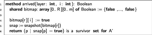
The BG-simulation code is shown in Figure 7.3. In the simulated computation, ![]() processes
processes ![]() share a two-dimensional memory mem[0..R][0..m]. At layer 0, the state of each
share a two-dimensional memory mem[0..R][0..m]. At layer 0, the state of each ![]() is its input. At layer
is its input. At layer ![]() , for
, for ![]() writes its current state to mem[r][i], then waits until the set of processes that have written to mem[r][·]constitutes a survivor set for
writes its current state to mem[r][i], then waits until the set of processes that have written to mem[r][·]constitutes a survivor set for ![]() .
. ![]() then takes a snapshot of mem[r][·], which becomes its new state. After completing
then takes a snapshot of mem[r][·], which becomes its new state. After completing ![]() steps,
steps, ![]() halts.
halts.

This computation is simulated by ![]() processes
processes ![]() . Each
. Each ![]() starts the protocol by proposing its own input value as the input initially written to memory by each
starts the protocol by proposing its own input value as the input initially written to memory by each ![]() (Line 8). Because the task is colorless, the simulation is correct even if simulated inputs are duplicated or omitted. Thus, if
(Line 8). Because the task is colorless, the simulation is correct even if simulated inputs are duplicated or omitted. Thus, if ![]() is the (colorless) input simplex of the
is the (colorless) input simplex of the ![]() processes, then each simulated
processes, then each simulated ![]() will take a value from
will take a value from ![]() as input, and altogether the simplex defined by the
as input, and altogether the simplex defined by the ![]() processes’ inputs will be a face of
processes’ inputs will be a face of ![]() .
.
In the main loop (Line 10), ![]() tries to complete a step on behalf of each
tries to complete a step on behalf of each ![]() in round-robin order. For each
in round-robin order. For each ![]() tries to resolve the value
tries to resolve the value ![]() wrote to memory during its previous layer (Line 13). If the resolution is successful,
wrote to memory during its previous layer (Line 13). If the resolution is successful, ![]() writes the resolved value on
writes the resolved value on ![]() ’s behalf to the simulated memory (Line 15). Although multiple processes may write to the same location on
’s behalf to the simulated memory (Line 15). Although multiple processes may write to the same location on ![]() ’s behalf, they all write the same value. When
’s behalf, they all write the same value. When ![]() observes that all
observes that all ![]() simulated layers have been written by simulated survivor sets (Line 16), then
simulated layers have been written by simulated survivor sets (Line 16), then ![]() returns the final state of some
returns the final state of some ![]() .
.
Otherwise, if ![]() did not return,
did not return, ![]() checks (Line 18) whether a survivor set of simulated processes for
checks (Line 18) whether a survivor set of simulated processes for ![]() has written values for that layer (Figure 7.4). If so, it takes a snapshot of those values and proposes that snapshot (after discarding process names, since the simulated protocol is colorless) as
has written values for that layer (Figure 7.4). If so, it takes a snapshot of those values and proposes that snapshot (after discarding process names, since the simulated protocol is colorless) as ![]() ’s state at the start of the next layer. Recall that adversaries
’s state at the start of the next layer. Recall that adversaries ![]() have minimum core size
have minimum core size ![]() . Thus, when
. Thus, when ![]() takes a snapshot in Line 19, at least
takes a snapshot in Line 19, at least ![]() entries in
entries in ![]() have been written, and hence the simulated execution is
have been written, and hence the simulated execution is ![]() -resilient.
-resilient.
Theorem 7.4.4
The BG simulation protocol is correct if ![]() , the maximum survivor set size for the adversaries
, the maximum survivor set size for the adversaries ![]() is less than or equal to
is less than or equal to ![]() .
.
Proof
At most ![]() of the
of the ![]() processors can fail in the unsafe zone of the safe agreement protocol, blocking at most
processors can fail in the unsafe zone of the safe agreement protocol, blocking at most ![]() out of the
out of the ![]() simulated processes, leaving
simulated processes, leaving ![]() simulated processes capable of taking steps. If
simulated processes capable of taking steps. If ![]() , there are always enough unblocked simulated processes to form a survivor set, ensuring that eventually some process completes each simulated layer.
, there are always enough unblocked simulated processes to form a survivor set, ensuring that eventually some process completes each simulated layer. ![]()
7.5 Conclusions
In this chapter we have once more seen the two faces of distributed computing: algorithmic and combinatorial. If we know a task is unsolvable in a certain model ![]() and we want to show it is unsolvable in another model
and we want to show it is unsolvable in another model ![]() , then it is natural to try to reduce model
, then it is natural to try to reduce model ![]() to model
to model ![]() instead of proving the impossibility result from scratch in
instead of proving the impossibility result from scratch in ![]() , especially if model
, especially if model ![]() seems more difficult to analyze than model
seems more difficult to analyze than model ![]() . The end result of a reduction is a simplicial map from protocols in
. The end result of a reduction is a simplicial map from protocols in ![]() to protocols in
to protocols in ![]() . We can produce such a simplicial map operationally using a protocol in
. We can produce such a simplicial map operationally using a protocol in ![]() , or we can show it exists, reasoning about the topological properties of the two models.
, or we can show it exists, reasoning about the topological properties of the two models.
The first reduction studied was for ![]() -set agreement. It was known that it is unsolvable in a (real) wait-free model
-set agreement. It was known that it is unsolvable in a (real) wait-free model ![]() even when
even when ![]() for
for ![]() processes. Proving directly that
processes. Proving directly that ![]() -set agreement is unsolvable in a (virtual)
-set agreement is unsolvable in a (virtual) ![]() -resilient model,
-resilient model, ![]() , when
, when ![]() seemed more complicated. Operationally, one assumes (for contradiction) that there is a
seemed more complicated. Operationally, one assumes (for contradiction) that there is a ![]() -set agreement protocol in
-set agreement protocol in ![]() . Then a generic protocol in
. Then a generic protocol in ![]() is used to simulate one by one the instructions of the protocol to obtain a solution for
is used to simulate one by one the instructions of the protocol to obtain a solution for ![]() -set agreement in
-set agreement in ![]() .
.
This operational approach has several benefits, including the algorithmic insights discovered while designing a simulation protocol, and its potential applicability for transforming solutions from one model of computation to another. However, to understand the possible reductions among a set of ![]() models of computation, we would have to devise
models of computation, we would have to devise ![]() explicit pair-wise simulations, each simulation intimately connected with the detailed structure of two models. Each simulation is likely to be a protocol of nontrivial complexity requiring a nontrivial operational proof.
explicit pair-wise simulations, each simulation intimately connected with the detailed structure of two models. Each simulation is likely to be a protocol of nontrivial complexity requiring a nontrivial operational proof.
By contrast, the combinatorial approach described in this chapter requires analyzing the topological properties of the protocol complexes for each of the ![]() models. Each such computation is a combinatorial exercise of the kind that has already been undertaken for many different models of computation. This approach is more systematic and, arguably, reveals more about the underlying structure of the models than explicit simulation algorithms. Indeed, in the operational approach, once a simulation is found, we also learn why it existed, but this new knowledge is not easy to formalize; it is hidden inside the correctness proof of the simulation protocol.
models. Each such computation is a combinatorial exercise of the kind that has already been undertaken for many different models of computation. This approach is more systematic and, arguably, reveals more about the underlying structure of the models than explicit simulation algorithms. Indeed, in the operational approach, once a simulation is found, we also learn why it existed, but this new knowledge is not easy to formalize; it is hidden inside the correctness proof of the simulation protocol.
We note that the definitions and constructions of this chapter, both the combinatorial and the operational, work only for colorless tasks. For arbitrary tasks, we can also define simulation in terms of maps between protocol complexes, but these maps require additional structure (they must be color-preserving, mapping real to virtual processes in a one-to-one way). See Chapter 14.
7.6 Chapter notes
Borowsky and Gafni [23] introduced the BG simulation to extend the wait-free set agreement impossibility result to the ![]() -resilient case. Later, Borowsky, Gafni, Lynch, and Rajsbaum [27] formalized and studied the simulation in more detail.
-resilient case. Later, Borowsky, Gafni, Lynch, and Rajsbaum [27] formalized and studied the simulation in more detail.
Borowsky, Gafni, Lynch, and Rajsbaum [27] identified the tasks for which the BG simulation can be used as the colorless tasks. This class of tasks was introduced in Herlihy and Rajsbaum [80,81], under the name convergence tasks, to study questions of decidability.
Borowsky and Gafni [25] and later Chaudhuri and Reiners [41] used the BG simulation to define and study the set agreement partial order [79]. Gafni and Kuznetsov [65] used the simulation to reduce solvability of colorless tasks under adversaries to wait-free solvability (see Exercise 7.3). Imbs and Raynal [97] consider a variant of the BG simulation where processes communicate through objects that can be used by at most ![]() processes to solve consensus as well as read-write registers. More broadly, BG simulation can be used to relate the power of different models to solve colorless tasks (see Exercise 7.10). Gafni, Guerraoui, and Pochon [60] use BG simulation to derive a lower bound on the round complexity of
processes to solve consensus as well as read-write registers. More broadly, BG simulation can be used to relate the power of different models to solve colorless tasks (see Exercise 7.10). Gafni, Guerraoui, and Pochon [60] use BG simulation to derive a lower bound on the round complexity of ![]() -set agreement in synchronous message-passing systems.
-set agreement in synchronous message-passing systems.
Gafni [62] extends the BG simulation to certain colored tasks, and Imbs and Raynal [96] discuss this simulation further.
The BG-simulation protocol we described is not layered (though the simulated protocol is layered). This protocol can be transformed into a layered protocol (see Chapter 14 and the next paragraph). Herlihy, Rajsbaum, and Raynal [87] present a layered safe agreement protocol (see Exercise 7.6).
Other simulations [26,67] address the computational power of layered models, where each shared object can be accessed only once. In Chapter 14 we consider such simulations between models with the same sets of processes, but different communication mechanisms.
Chandra [35] uses a simulation argument to prove the equivalence of ![]() -resilient and wait-free consensus protocols using shared objects.
-resilient and wait-free consensus protocols using shared objects.
Exercise 7.1 is based on Afek, Gafni, Rajsbaum, Raynal, and Travers [4], where reductions between simultaneous consensus and set agreement are described.
7.7 Exercises
Exercise 7.1
In the ![]() -simultaneous consensus task a process has an input value for
-simultaneous consensus task a process has an input value for ![]() independent instances of the consensus problem and is required to decide in at least one of them. A process decides a pair
independent instances of the consensus problem and is required to decide in at least one of them. A process decides a pair ![]() , where
, where ![]() is an integer between
is an integer between ![]() and
and ![]() , and if two processes decide pairs
, and if two processes decide pairs ![]() and
and ![]() , with
, with ![]() , then
, then ![]() , and
, and ![]() was proposed by some process to consensus instance
was proposed by some process to consensus instance ![]() and
and ![]() . State formally the
. State formally the ![]() -simultaneous consensus problem as a colorless task, and draw the input and output complex for
-simultaneous consensus problem as a colorless task, and draw the input and output complex for ![]() . Show that
. Show that ![]() -set agreement and
-set agreement and ![]() -simultaneous consensus (both with sets of possible input values of the same size) are wait-free equivalent (there is a read-write layered protocol to solve one using objects that implement the other).
-simultaneous consensus (both with sets of possible input values of the same size) are wait-free equivalent (there is a read-write layered protocol to solve one using objects that implement the other).
Exercise 7.3
Using the BG simulation, show that a colorless task is solvable by an ![]() -resilient layered snapshot protocol if and only if it is solvable by a
-resilient layered snapshot protocol if and only if it is solvable by a ![]() -resilient layered immediate snapshot protocol, where
-resilient layered immediate snapshot protocol, where ![]() is the size of the minimum core of
is the size of the minimum core of ![]() (and in particular by a
(and in particular by a ![]() process wait-free layered immediate snapshot protocol).
process wait-free layered immediate snapshot protocol).
Exercise 7.8
In the BG simulation, what is the maximum number of snapshots a process can take to simulate an ![]() -round layered protocol?
-round layered protocol?
Exercise 7.9
For the BG simulation, show that the map ![]() , carrying final views of the simulating protocol to final views of the simulated protocol, is onto: every simulated execution is produced by some simulating execution.
, carrying final views of the simulating protocol to final views of the simulated protocol, is onto: every simulated execution is produced by some simulating execution.
Exercise 7.10
Consider Exercise 5.6, where we are given a “black box” object that solves ![]() -set agreement for
-set agreement for ![]() processes. Define a wait-free layered model that has access to any number of such boxes as well as read-write registers. Use simulations to find to which of the models considered in this chapter it is equivalent in the sense that the same colorless tasks can be solved.
processes. Define a wait-free layered model that has access to any number of such boxes as well as read-write registers. Use simulations to find to which of the models considered in this chapter it is equivalent in the sense that the same colorless tasks can be solved.
Exercise 7.11
We have seen that it is undecidable whether a colorless task has a ![]() -resilient layered snapshot protocol for
-resilient layered snapshot protocol for ![]() (Corollary 5.6.12). Use simulations to conclude undecidability results in other models. More generally, suppose that in a virtual model
(Corollary 5.6.12). Use simulations to conclude undecidability results in other models. More generally, suppose that in a virtual model ![]() colorless task solvability is undecidable. State a theorem that allows us to conclude undecidability in a real model
colorless task solvability is undecidable. State a theorem that allows us to conclude undecidability in a real model ![]() .
.