| 22 | Complex Numbers |
Long ago, humankind didn’t accept fractions, only whole numbers could be counted. Then people could count only positive quantities, because negative numbers were impossible for them to imagine. After negative numbers became familiar, the square roots of negative real numbers were defined, producing imaginary numbers. The resulting quantities were combined with real numbers to get complex numbers. You were introduced to imaginary and complex numbers earlier in this book. Now, you’ll learn how to work with these numbers and find out how they can be useful in solving problems that would be much more difficult without them.
IMAGINARY QUANTITIES
Think of all the real numbers as points on a straight line. A certain point is assigned the value 0. Then positive numbers go in one direction from that point, and negative numbers are expressed in a 180° reversal from the positive numbers. For example, if the positive numbers go out on a straight line toward the right, the negative numbers go toward the left. Imaginary numbers can then be placed on another line that runs upward for positive and downward for negative.
Figure 22-1 shows geometric representations of the real (A) and imaginary numbers (B) when portrayed on straight lines. This can help you visualize the relationship between the real numbers and the imaginary numbers (C). Multiplying any number by −1 in the plane of Fig. 22-1C produces rotation through 180° Multiplying by −1 again produces another rotation through 180°, which brings you back to the original number. Minus times minus equals plus, remember!

Figure 22-1
At A, the real number line. At B, the positive imaginary number half-line (i) is perpendicular to the real number line. At C, the positive and negative imaginary numbers (+i and −i) lie on a complete geometric line perpendicular to the real number line.
You don’t need to worry about whether the rotation is clockwise or counterclockwise when you multiply by −1. You reverse the direction, that’s all! But when you multiply a number by the unit imaginary operator i, which represents the positive square root of −1, things are a little more interesting. Multiplying by i is the equivalent of rotating counterclockwise through 90° in a geometric representation such as the one shown in Fig. 22-1C.
Figure 22-2 shows what happens when you repeatedly multiply a positive real number by i. When you first multiply, you get a positive imaginary number (Fig. 22-2A). When you multiply by i twice, you rotate through 180° as shown in Fig. 22-2B. When you multiply by i three times, the rotation is 270° (Fig. 22-2C). If you multiply by i four times, you go around in a complete circle and return to the original number (Fig. 22-2D).

Figure 22-2
At A, multiplication of a real number by i. At B, multiplication by i×i or i2. At C, multiplication by i×i×i or i3. At D, multiplication by i×i× i×i or i4.
Multiplying repeatedly by i works the same way no matter what number you start out with. You can begin with a negative real, a positive imaginary, a negative imaginary, or even the sum of a real number and an imaginary one. Each multiplication by i always turns the complex number vector (a ray connecting the origin with the point in the coordinate plane representing the number) counterclockwise through 90° The length of the vector does not change unless you multiply a number by some quantity ib, where b is a real number. In that case, the vector length is multiplied by b, and it rotates through 90° also. For example, if you multiply something by i2, the vector turns 90° counterclockwise and becomes twice as long; if you multiply by i/12 or i(1/12), the vector turns 90° counterclockwise and becomes 1/12 as long.
THE COMPLEX NUMBER PLANE
The set of rectangular coordinates shown in Fig. 22-2A through D is known as the complex number plane, in which you can plot quantities that are part real and part imaginary. The real part is expressed toward the right for positive and toward the left for negative. The imaginary part goes upward for positive and downward for negative. Any point in the plane, representing a unique complex number, can be expressed as an ordered pair (a,ib) or written algebraically as a + ib, where a and b are real numbers and i is the unit imaginary number.
If a = 0, a complex number is called pure imaginary. If b = 0, a complex number is called pure real. If both parts are positive, the quantity is in the first quadrant of the complex number plane. If the real part is negative and the imaginary part is positive, the quantity is in the second quadrant. If both parts are negative, the quantity is in the third quadrant. If the real part is positive but the imaginary part is negative, the quantity is in the fourth quadrant.
MULTIPLYING COMPLEX QUANTITIES
Here is a geometric method by which you can multiply complex numbers. Suppose you have two complex quantities that can be portrayed both in rectangular coordinates as real and imaginary parts and in mathematician’s polar coordinates as a vector magnitude and a direction angle. In Fig. 22-3, two complex quantities a + ib and c + id are set out, each beginning at the positive real number axis. In polar form these complex numbers are (θ,r) and (φ,s) respectively. Complete the triangles formed by these vectors, the real axis, and vertical lines running from the plotted points down to the real axis. These triangles are shaded in the diagram. Beginning at the magnitude of the first quantity and multiplying each part of the second by the magnitude of the first, you can erect a third, unshaded triangle. This triangle brings you to the product, in magnitude and angle, or it can be read in rectangular coordinates as real and imaginary parts. Study the calculations next to the diagram to see how the quantities that appear in the algebra are reproduced in coordinate geometry.

Figure 22-3
Geometric representation of the product of two complex quantities.
A simpler situation exists when you want to square a complex number. In this case, you multiply the magnitude of the original vector by itself, and then you rotate the vector counterclockwise by an angle equal to its original angle with respect to the positive real number axis. That is, you double its counterclockwise direction angle. For example, if you want to square a complex number with a vector length of 4 that points 70° counterclockwise from the positive real axis, you increase the vector length to 42, or 16, and you double its angle to 70° · 2, or 140°. If you want to square the complex number 3 + i4, you can draw it on a coordinate plane and figure out that it has a length of exactly 5 (from the Pythagorean theorem) and points at an angle of arctan (4/3), or approximately 53° counterclockwise from the positive real axis. Squaring this gives you a vector with a length of 52, or 25, and an angle of approximately 53° · 2, or 106°.
THREE CUBE ROOT EXAMPLES
Now consider the cube roots of 1. You know that within the set of real numbers, the cube root of 1 is equal to 1, because 1 · 1 · 1 = 1. But there are nonreal, complex number roots as well. One of these is a vector with a magnitude of 1 unit, in the second quadrant at an angle of 120° counterclockwise from the positive real number axis. Squaring this puts the product in the third quadrant, at 240°. Cubing it verifies it as a cube root, by turning to 360° so the vector ends up on the positive part of the real number axis with the length still at 1 unit. This is shown in Fig. 22-4A.
Now suppose that you start with a vector of length 1 unit in the third quadrant at 240° Multiply this by itself to get the square at 480° and then multiply again by the original vector to get the cube when it is at 720° or two complete revolutions (Fig. 22-4B). This shows that the quantity you began with is the cube root of 1.
Finally, imagine that you start with a vector of length 1 unit along the positive real axis, but think of it as oriented at 360° Squaring this takes you around one complete circle to 720° Then, multiplying again by the original vector, you go another complete circle to 1080° so you end up with 1 again. This is the “conventional” or real number cube root of 1 that you usually think of (Fig. 22-4C).

Figure 22-4
The three cube roots of 1. At A and B, the roots are complex and non-real. At C, the root is pure real and equal to 1.
How are quantities with magnitudes other than 1 represented? As an example, look at the cube root of 8. Using the same method as before, the first cube root of 8 is −1 + i(3½), which is at an angle of 120° Then multiply that quantity by itself and simplify, getting − 2 − i2(3½). Multiplying by the original quantity again returns the answer to 8; the imaginary part disappears to prove that the cube root is correct. This is shown in Fig. 22-5.
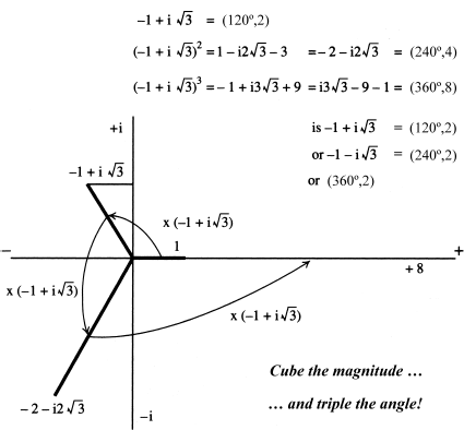
Figure 22-5
The three cube roots of 8. Two are complex and nonreal; the third is pure real and equal to 2.
Now look at the cube roots of −1. The complex, nonreal root in the first quadrant has a magnitude of 1 and is at 60° Squaring it puts the product in the second quadrant at 120° Multiplying again verifies it as a cube root, by turning to 180° so it ends up on the negative real axis with a length of 1 unit. This process is shown in Fig. 22-6. Another cube root of −1 has a length of 1 unit and is oriented at an angle of 180° counterclockwise from the positive real axis. This is the root you usually think of; it is pure real and is equal to −1. Another complex, nonreal cube root of −1 has a length of 1 unit and is oriented at an angle of 300β counterclockwise from the positive real number axis.

Figure 22-6
Geometric construction and algebra describing one of the complex, non-real cube roots of −1.
When you cube it, you get a vector at an angle of 900°. If you subtract 360° from this twice, you can see that it is in the same direction as 180° which lies exactly along the negative real axis.
RECIPROCAL OF A COMPLEX QUANTITY
If the vector representing a complex number a + ib has magnitude r that is greater than 1, its reciprocal has magnitude 1/r, which is of course less than 1. An example of this is shown in Fig. 22-7. The triangular portion of the shaded area above the real number axis uses unit magnitude on the positive real axis for its base, and the magnitude r of the quantity a + ib for its top side. Scaling this area down to make the longest side fit unit magnitude on the positive real axis, the side that was 1 in the bigger triangle is now the reciprocal of the original complex quantity, in both magnitude and polar angle. This is represented by the part of the shaded area below the real axis.

Figure 22-7
Geometric representation of the reciprocal of a complex quantity.
The algebra in the figure shows how to calculate these values. When you have the quantity a + ib in the denominator of an expression, it presents a problem that is rather difficult to work out directly. However, if you multiply both the numerator and the denominator of such a fraction by a − ib, the denominator becomes the sum of two squares, which is a real number. It’s always a lot easier to divide by a real number than it is to divide by a complex number!
In the study and use of complex quantities, the quantity a − ib is called the conjugate of a + ib, and vice versa. The product of two complex conjugates is always a pure real number.
DIVISION OF COMPLEX QUANTITIES
Figure 22-8 is a geometric rendition of how a complex number can be divided by another complex number. From the actual size of the divisor (the shaded area in the upper left part of the figure), change the magnitude of the longest side to fit the longest side of the dividend, maintaining its shape or proportion. The quotient is then the side of the proportionate area of the divisor that was unit positive on the real axis before it was reduced. As the upper right portion of the figure shows, the angle of the quotient is found by subtracting the angle of the divisor from the angle of the dividend (θ−φ). The magnitudes are simply divided by each other. This is represented by r/s in the calculations in the lower part of Fig. 22-8.

Figure 22-8
Geometric representation of the quotient of two complex quantities.
RATIONALIZATION
In complex number algebra, rationalization is the equivalent of the simplification of fractions in ordinary algebra. A complex quantity is the sum of a real number and an imaginary number. Complex quantities can, as numerators, share the same denominator as a matter of convenience. But the denominator in any such expression should always be pure real. This makes complex number fractions much easier to work with.
Consider a simplification that consists of two complex quantities multiplied together in the numerator and two more multiplied together in the denominator, as generalized in the upper part of Fig. 22-9. When the quantities are multiplied, the numerator and denominator can each be simplified to single real and imaginary parts. To rationalize, the numerator and denominator are each multiplied by the conjugate of the denominator, so only the numerator contains both real and imaginary parts. If desired, the whole quantity can be written separately as a real part and as an imaginary part.

Figure 22-9
The general process of rationalization, along with a specific example.
A specific example of rationalization, using actual numbers instead of variables, is shown in the lower portion of Fig. 22-9.
CHECKING RESULTS
It is easy to make mistakes when handling complex numbers, even if you use a calculator! Often, the numbers happen to be convenient for making some relatively simple checks. In the example of Fig. 22-10, the first factor in the numerator has the same vector magnitude as the first factor in the denominator, even though the two complex numbers themselves are different. One factor is 3 + i4 and the other is 4 + i3. The vector magnitude of either one is equal to 5. Because of this, the whole expression will have the same magnitude if these two factors are removed; only the angle is changed. If you like, go ahead and check to see that this is really true.

Figure 22-10
Division of complex numbers can be checked by comparing vector magnitudes.
OPERATION SUMMARY
Here is a summary of facts you should remember about combining quantities in complex number algebra using geometric polar coordinate representations.
• When you want to add or subtract two complex numbers, you must always work on the real and imaginary parts separately. There’s no polar equivalent that works out conveniently.
• When you want to multiply two complex numbers, multiply the vector magnitudes and add the polar angles.
• When you want to divide two complex numbers, divide the vector magnitude of the numerator by the vector magnitude of the denominator, and subtract the polar angle of the denominator from the polar angle of the numerator.
• When you want to raise a complex number to a real power, take the real power of the vector magnitude, and multiply the polar angle by the value of the real power.
• When you want to find a real root of a complex number, take the root of the vector magnitude, and divide the polar angle by the value (or index) of the real root.
USE OF A COMPLEX PLANE
The invention of complex numbers, and the evolution of the algebra that goes with them, led mathematicians and scientists to use the complex number coordinate plane in various ways. In the conventional graphic representation of quantities—the Cartesian plane or xy plane—the independent variable (usually x) is expressed horizontally, and the dependent variable (usually y) is expressed vertically.
In complex number mathematics, the independent variable requires a plane to be completely represented. The real part is measured left or right, but the imaginary part is measured at right angles to it. The direction for the dependent variable is vertical. This results in a variant of xyz space, in which x is replaced by the real number part x of a complex number, y is replaced by the imaginary part iz, and z is replaced by the dependent variable y, which is a function of the complex number x + iz. Figure 22-11 shows how this system is put together.

Figure 22-11
At A, the traditional xy-plane. At B, a complex plane as the basis for the independent variable in a real-number function of a complex variable. At C, a three-dimensional set of rectangular coordinates for plotting real-number functions of complex variables.
Figure 22-12 illustrates a qualitative example of a real number function of a complex variable, graphed in the system of coordinates from Fig. 22-11C. For each point on the complex number plane defined by the axes x and iz, the value of y, which is a real number dependent variable, is plotted vertically. At a point where the denominator is zero, the value of y “goes to infinity” or “blows up.” This is called a pole of the graph. Where the numerator goes to zero, the value of y is 0. This is called a zero of the graph. Not all graphs of this kind have poles or zeros.

Figure 22-12
An example of a three-dimensional graph representing a real-number function of a complex variable.
ROOTS BY COMPLEX QUANTITIES
You can often simplify the process of finding roots by using complex quantities. For example, you know that 32 has a 5th root that is equal to 2, because 25 = 32. But your advancing knowledge of mathematics ought to help you realize that 32 has four more 5 th roots. These roots all have magnitude 2 in the complex polar plane, with angles that divide a full 360° revolution into five equal parts (Fig. 22-13). Using the cosines and sines of the angles shown, you can derive the complex roots in the form a + ib from the following expressions:


Figure 22-13
The five 5th roots of 32, shown as vectors in the com plex polar plane.
The first four of these roots are complex. The last is pure real, as you can determine by working out the cosine and sine values or by looking at Fig. 22-13.
QUESTIONS AND PROBLEMS
This is an open-book quiz. You may refer to the text in this chapter (and earlier ones, too, if you want) when figuring out the answers. Take your time! Consider all values given as exact, so you don’t have to worry about significant figures. The correct answers are in the back of the book. Note: In these problems, the square root of −1 is denoted by j, not i. You should get used to this notation because it is commonly used by engineers.
1. Find the product (0.6 + j0.8)(0.8 + j0.6). Verify that the result is pure imaginary and that its vector has a magnitude of 1.
2. Square each of the factors in Prob. 1. Then multiply the resulting complex numbers together, and verify that the product is pure real and that its vector has a magnitude of 1.
3. Solve the following quadratic equations. Include all imaginary, complex, and real solutions.
(a) x2 − 2x + 2 = 0
(b) x2 − 2x + 10 = 0
(c) 13x2 − 4x + 1 = 0
(d) x2 − j2x − 10 = 0
(e) x2 − j2x − 8 = 0
4. Find the six 6th roots of 64. Express the coefficients in decimal form to three significant digits. Plot the corresponding vectors on the complex plane.
5. Find the ten 10th roots of 1,024. Express the coefficients in decimal form to three significant digits. Plot the corresponding vectors on the complex plane.
6. Find the nine 9th roots of 512. Express the coefficients in decimal form to three significant digits. Plot the corresponding vectors on the complex plane.
7. Refer to Fig. 22-14. Find the sum of the two complex numbers shown.

Figure 22-14
Illustration for problems 7 through 14.
8. Plot the vector denoting the sum of the complex numbers shown in Fig. 22-14.
9. Find the product of the complex numbers shown in Fig. 22-14.
10. Plot the vector denoting the product of the complex numbers shown in Fig. 22-14.
11. Divide the complex number shown as a second-quadrant vector by the complex number shown as a third-quadrant vector in Fig. 22-14. Express the coefficients in decimal form to three significant digits.
12. Plot the vector denoting the quotient you found in Prob. 11.
13. Divide the complex number shown as a third-quadrant vector by the complex number shown as second-quadrant vector in Fig. 22-14. Express the coefficients in decimal form to three significant digits.
14. Plot the vector denoting the quotient you found in Prob. 13.
15. Refer to Fig. 22-15. Find the product of these two complex numbers.

Figure 22-15
Illustration for problems 15 through 17.
16. Plot, in polar coordinates, the vector denoting the product of the complex numbers shown in Fig. 22-15.
17. Convert the product vector from Probs. 15 and 16 to the form a + jb, where a and b are real numbers and j is the positive square root of −1. Express the coefficients to three significant digits.
..................Content has been hidden....................
You can't read the all page of ebook, please click here login for view all page.