
Chapter 9
Audio Coding
For transmission and storage of audio signals, different methods for compressing data have been investigated besides the pulse code modulation representation. The requirements of different applications have led to a variety of audio coding methods which have become international standards. In this chapter basic principles of audio coding are introduced and the most important audio coding standards discussed. Audio coding can be divided into two types: lossless and lossy. Lossless audio coding is based on a statistical model of the signal amplitudes and coding of the audio signal (audio coder). The reconstruction of the audio signal at the receiver allows a lossless resynthesis of the signal amplitudes of the original audio signal (audio decoder). On the other hand, lossy audio coding makes use of a psychoacoustic model of human acoustic perception to quantize and code the audio signal. In this case only the acoustically relevant parts of the signal are coded and reconstructed at the receiver. The samples of the original audio signal are not exactly reconstructed. The objective of both audio coding methods is a data rate reduction or data compression for transmission or storage compared to the original PCM signal.
9.1 Lossless Audio Coding
Lossless audio coding is based on linear prediction followed by entropy coding [Jay84] as shown in Fig. 9.1:
- Linear Prediction. A quantized set of coefficients P for a block of M samples is determined which leads to an estimate
 of the input sequence x(n). The aim is to minimize the power of the difference signal d(n) without any additional quantization errors, i.e. the word-length of the signal
  must be equal to the word-length of the input. An alternative approach [Han98, Han01] quantizes the prediction signal
  such that the word-length of the difference signals d(n) remains the same as the input signal word-length. Figure 9.2 shows a signal block x(n) and the corresponding spectrum |X(f)|. Filtering the input signal with the predictor filter transfer function P(z) delivers the estimate
  . Subtracting input and prediction signal yields the prediction error d(n), which is also shown in Fig. 9.2 and which has a considerably lower power compared to the input power. The spectrum of this prediction error is nearly white (see Fig. 9.2, lower right). The prediction can be represented as a filter operation with an analysis transfer function HA(z) = 1 − P(z) on the coder side.

Figure 9.1 Lossless audio coding based on linear prediction and entropy coding.
- Entropy Coding. Quantization of signal d(n) due to the probability density function of the block. Samples d(n) of greater probability are coded with shorter data words, whereas samples d(n) of lesser probability are coded with longer data words [Huf52].
- Frame Packing. The frame packing uses the quantized and coded difference signal and the coding of the M coefficients of the predictor filter P(z) of order M.
- Decoder. On the decoder side the inverse synthesis transfer function HS(z) =
 reconstructs the input signal with the coded difference samples and the M filter coefficients. The frequency response of this synthesis filter represents the spectral envelope shown in the upper right part of Fig. 9.2. The synthesis filter shapes the white spectrum of the difference (prediction error) signal with the spectral envelope of the input spectrum.
The attainable compression rates depend on the statistics of the audio signal and allow a compression rate of up to 2 [Bra92, Cel93, Rob94, Cra96, Cra97, Pur97, Han98, Han01, Lie02, Raa02, Sch02]. Figure 9.3 illustrates examples of the necessary word-length for lossless audio coding [Blo95, Sqa88]. Besides the local entropy of the signal (entropy computed over a block length of 256), results for linear prediction followed by Huffman coding [Huf52] are presented. Huffman coding is carried out with a fixed code table [Pen93] and a power-controlled choice of adapted code tables. It is observed from Fig. 9.3 that for high signal powers, a reduction in word-length is possible if the choice is made from several adapted code tables. Lossless compression methods are used for storage media with limited word-length (16 bits in CD and DAT) which are used for recording audio signals of higher word-lengths (more than 16 bits). Further applications are in the transmission and archiving of audio signals.

Figure 9.2 Signals and spectra for linear prediction.
9.2 Lossy Audio Coding
Significantly higher compression rates (of factor 4 to 8) can be obtained with lossy coding methods. Psychoacoustic phenomena of human hearing are used for signal compression. The fields of application have a wide range, from professional audio like source coding for DAB to audio transmission via ISDN and home entertainment like DCC and MiniDisc.
An outline of the coding methods [Bra94] is standardized in an international specification ISO/IEC 11172-3 [ISO92], which is based on the following processing (see Fig. 9.4):
- subband decomposition with filter banks of short latency time;
- calculation of psychoacoustic model parameters based on short-time FFT;
- dynamic bit allocation due to psychoacoustic model parameters (signal-to-mask ratio SMR);
- quantization and coding of subband signals;
- multiplex and frame packing.

Figure 9.3 Lossless audio coding (Mozart, Stravinsky): word-length in bits versus time (entropy - -, linear prediction with Huffman coding—).
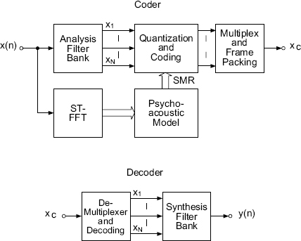
Figure 9.4 Lossy audio coding based on subband coding and psychoacoustic models.
Owing to lossy audio coding, post-processing of such signals or several coding and decoding steps is associated with some additional problems. The high compression rates justify the use of lossy audio coding techniques in applications like transmission.
9.3 Psychoacoustics
In this section, basic principles of psychoacoustics are presented. The results of psychoacoustic investigations by Zwicker [Zwi82, Zwi90] form the basis for audio coding based on models of human perception. These coded audio signals have a significantly reduced data rate compared to the linearly quantized PCM representation. The human auditory system analyzes broad-band signals in so-called critical bands. The aim of psychoacoustic coding of audio signals is to decompose the broad-band audio signal into subbands which are matched to the critical bands and then perform quantization and coding of these subband signals [Joh88a, Joh88b, Thei88]. Since the perception of sound below the absolute threshold of hearing is not possible, subband signals below this threshold need neither be coded nor transmitted. In addition to the perception in critical bands and the absolute threshold, the effects of signal masking in human perception play an important role in signal coding. These are explained in the following and their application to psychoacoustic coding is discussed.
9.3.1 Critical Bands and Absolute Threshold
Critical Bands. Critical bands as investigated by Zwicker are listed in Table 9.1.
Table 9.1 Critical bands as given by Zwicker [Zwi82].
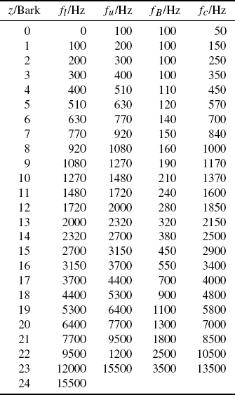
A transformation of the linear frequency scale into a hearing-adapted scale is given by Zwicker [Zwi90] (units of z in Bark):

The individual critical bands have bandwidths

Absolute Threshold. The absolute threshold LTq (threshold in quiet) denotes the curve of sound pressure level L [Zwi82] versus frequency, which leads to the perception of a sinusoidal tone. The absolute threshold is given by [Ter79]:
Below the absolute threshold, no perception of signals is possible. Figure 9.5 shows the absolute threshold versus frequency. Band-splitting in critical bands and the absolute threshold allow the calculation of an offset between the signal level and the absolute threshold for every critical band. This offset is responsible for choosing appropriate quantization steps for each critical band.

Figure 9.5 Absolute threshold (threshold in quiet).
9.3.2 Masking
For audio coding the use of sound perception in critical bands and absolute threshold only is not sufficient for high compression rates. The basis for further data reduction are the masking effects investigated by Zwicker [Zwi82, Zwi90]. For band-limited noise or a sinusoidal signal, frequency-dependent masking thresholds can be given. These thresholds perform masking of frequency components if these components are below a masking threshold (see Fig. 9.6). The application of masking for perceptual coding is described in the following.

Figure 9.6 Masking threshold of band-limited noise.
Calculation of Signal Power in Band i. First, the sound pressure level within a critical band is calculated. The short-time spectrum X(k) = DFT[x(n)] is used to calculate the power density spectrum
with the help of an N-point FFT. The signal power in band i is calculated by the sum

from the lower frequency up to the upper frequency of critical band i. The sound pressure level in band i is given by LS(i) = 10 log10 Sp(i).
Absolute Threshold. The absolute threshold is set such that a 4 kHz signal with peak amplitude ±1 LSB for a 16-bit representation lies at the lower limit of the absolute threshold curve. Every masking threshold calculated in individual critical bands, which lies below the absolute threshold, is set to a value equal to the absolute threshold in the corresponding band. Since the absolute threshold within a critical band varies for low and high frequencies, it is necessary to make use of the mean absolute threshold within a band.
Masking Threshold. The offset between signal level and the masking threshold in critical band i (see Fig. 9.7) is given by [Hel72]
where α denotes the tonality index and av is the masking index. The masking index [Kap92] is given by
As an approximation,
can be used [Joh88a, Joh88b]. If a tone is masking a noise-like signal (α = 1), the threshold is set 14.5 + i dB below the value of LS(i). If a noise-like signal is masking a tone (α = 0), the threshold is set 5.5 + i dB below LS(i). In order to recognize a tonal or noise-like signal within a certain number of samples, the spectral flatness measure SFM is estimated. The SFM is defined by the ratio of the geometric to arithmetic mean value of Sp(i) as

The SFM is compared with the SFM of a sinusoidal signal (definition SFMmax = −60 dB) and the tonality index is calculated [Joh88a, Joh88b] by
SFM = 0 dB corresponds to a noise-like signal and leads to α = 0, whereas an SFM=75 dB gives a tone-like signal (α = 1). With the sound pressure level LS(i) and the offset O(i) the masking threshold is given by
Masking across Critical Bands. Masking across critical bands can be carried out with the help of the Bark scale. The masking threshold is of a triangular form which decreases at S1 dB per Bark for the lower slope and at S2 dB per Bark for the upper slope, depending on the sound pressure level Li and the center frequency fci in band i (see [Ter79]) according to

An approximation of the minimum masking within a critical band can be made using Fig. 9.8 [Thei88, Sauv90]. Masking at the upper frequency fui in the critical band i is responsible for masking the quantization noise with approximately 32 dB using the lower masking threshold that decreases by 27 dB/Bark. The upper slope has a steepness which depends on the sound pressure level. This steepness is lower than the steepness of the lower slope. Masking across critical bands is presented in Fig. 9.9. The masking signal in critical band i − 1 is responsible for masking the quantization noise in critical band i as well as the masking signal in critical band i. This kind of masking across critical bands further reduces the number of quantization steps within critical bands.
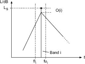
Figure 9.7 Offset between signal level and masking threshold.
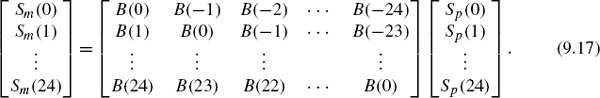
An analytical expression for masking across critical bands [Schr79] is given by
Δi denotes the distance between two critical bands in Bark. Expression (9.15) is called the spreading function. With the help of this spreading function, masking of critical band i by critical band j can be calculated [Joh88a, Joh88b] with abs (i − j) ≤ 25 such that


Figure 9.8 Masking within a critical band.

Figure 9.9 Masking across critical bands.
The masking across critical bands can therefore be expressed as a matrix operation given by
A renewed calculation of the masking threshold with (9.16) leads to the global masking threshold
For a clarification of the single steps for a psychoacoustic based audio coding we summarize the operations with exemplified analysis results:
- calculation of the signal power Sp(i) in critical bands → LS(i) in dB (Fig. 9.10a);
- calculation of masking across critical bands Tm(i) → LTm(i) in dB (Fig. 9.10b);
- masking with tonality index → LTm(i) in dB (Fig. 9.10c);
- calculation of global masking threshold with respect to threshold in quiet LTq → LTm, abs(i) in dB (Fig. 9.10d).
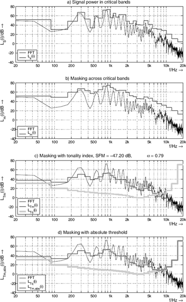
Figure 9.10 Stepwise calculation of psychoacoustic model.
With the help of the global masking threshold LTm, abs(i) we calculate the signal-to-mask ratio
per Bark band. This signal-to-mask ratio defines the necessary number of bits per critical band, such that masking of quantization noise is achieved. For the given example the signal power and the global masking threshold are shown in Fig. 9.11a. The resulting signal-to-mask ratio SMR(i) is shown in Fig. 9.11b. As soon as SMR(i) > 0, one has to allocate bits to the critical band i. For SMR(i) < 0 the corresponding critical band will not be transmitted. Figure 9.12 shows the masking thresholds in critical bands for a sinusoid of 440 Hz. Compared to the first example, the influence of masking thresholds across critical bands is easier to observe and interpret.

Figure 9.11 Calculation of the signal-to-mask ratio SMR.
9.4 ISO-MPEG-1 Audio Coding
In this section, the coding method for digital audio signals is described which is specified in the standard ISO/IEC 11172-3 [ISO92]. The filter banks used for subband decomposition, the psychoacoustic models, dynamic bit allocation and coding are discussed. A simplified block diagram of the coder for implementing layers I and II of the standard is shown in Fig. 9.13. The corresponding decoder is shown in Fig. 9.14. It uses the information from the ISO-MPEG1 frame and feeds the decoded subband signals to a synthesis filter bank for reconstructing the broad-band PCM signal. The complexity of the decoder is, in contrast to the coder, significantly lower. Prospective improvements of the coding method are being made entirely for the coder.

Figure 9.12 Calculation of psychoacoustic model for a pure sinusoid with 440 Hz.

Figure 9.13 Simplified block diagram of an ISO-MPEG1 coder.
9.4.1 Filter Banks
The subband decomposition is done with a pseudo-QMF filter bank (see Fig. 9.15). The theoretical background is found in the related literature [Rot83, Mas85, Vai93]. The broadband signal is decomposed into M uniformly spaced subbands. The subbands are processed further after a sampling rate reduction by a factor of M. The implementation of an ISO-MPEG1 coder is based on M = 32 frequency bands. The individual band-pass filters H0(z)…HM−1(z) are designed using a prototype low-pass filter H(z) and frequencyshifted versions. The frequency shifting of the prototype with cutoff frequency π/2M is done by modulating the impulse response h(n) with a cosine term [Bos02] according to

Figure 9.14 Simplified block diagram of an ISO-MPEG1 decoder.
with k = 0,…, 31 and n = 0,…, 511. The band-pass filters have bandwidth π/M. For the synthesis filter bank, corresponding filters F0(z)…FM−1(z) give outputs which are added together, resulting in a broad-band PCM signal. The prototype impulse response with 512 taps, the modulated band-pass impulse responses, and the corresponding magnitude responses are shown in Fig. 9.16. The magnitude responses of all 32 band-pass filters are also shown. The overlap of neighboring band-pass filters is limited to the lower and upper filter band. This overlap reaches up to the center frequency of the neighboring bands. The resulting aliasing after downsampling in each subband will be canceled in the synthesis filter bank. The pseudo-QMF filter bank can be implemented by the combination of a polyphase filter structure followed by a discrete cosine transform [Rot83, Vai93, Kon94].
To increase the frequency resolution, layer III of the standard decomposes each of the 32 subbands further into a maximum of 18 uniformly spaced subbands (see Fig. 9.17). The decomposition is carried out with the help of an overlapped transform of windowed subband samples. The method is based on a modified discrete cosine transform, also known as the TDAC filter bank (Time Domain Aliasing Cancellation) and MLT (Modulated Lapped Transform). An exact description is given in [Pri87, Mal92]. This extended filter bank is referred to as the polyphase/modified discrete cosine transform (MDCT) hybrid filter bank [Bra94]. The higher frequency resolution enables a higher coding gain but has the disadvantage of a worse time resolution. This is observed for impulse-like signals. In order to minimize these artifacts, the number of subbands per subband can be altered from 18 down to 6. Subband decompositions that are matched to the signal can be obtained by specially designed window functions with overlapping transforms [Edl89, Edl95]. The equivalence of overlapped transforms and filter banks is found in [Mal92, Glu93, Vai93, Edl95, Vet95].

Figure 9.15 Pseudo-QMF filter bank.
9.4.2 Psychoacoustic Models
Two psychoacoustic models have been developed for layers I to III of the ISO-MPEG1 standard. Both models can be used independently of each other for all three layers. Psychoacoustic model 1 is used for layers I and II, whereas model 2 is used for layer III. Owing to the numerous applications of layers I and II, we discuss psychoacoustic model 1 in this subsection.
Bit allocation in each of the 32 subbands is carried out using the signal-to-mask ratio SMR(i). This is based on the minimum masking threshold and the maximum signal level within a subband. In order to calculate this ratio, the power density spectrum is estimated with the help of a short-time FFT in parallel with the analysis filter bank. As a consequence, a higher frequency resolution is obtained for estimating the power density spectrum in contrast to the frequency resolution of the 32-band analysis filter bank. The signal-to-mask ratio for every subband is determined as follows:
- Calculate the power density spectrum of a block of N samples using FFT. After windowing a block of N = 512 (N = 1024 for layer II) input samples, the power density spectrum

Figure 9.16 Impulse responses and magnitude responses of pseudo-QMF filter bank.

Figure 9.17 Polyphase/MDCT hybrid filter bank.
is calculated. Then the window h(n) is displaced by 384 (12 · 32) samples and the next block is processed.
- Determine the sound pressure level in every subband. The sound pressure level is derived from the calculated power density spectrum and by calculating a scaling factor in the corresponding subband as given by
For X(k), the maximum of the spectral lines in a subband is used. The scaling factor SCF(i) for subband i is calculated from the absolute value of the maximum of 12 consecutive subband samples. A nonlinear quantization to 64 levels is carried out (layer I). For layer II, the sound pressure level is determined by choosing the largest of the three scaling factors from 3 · 12 subband samples.
- Consider the absolute threshold. The absolute threshold LTq(m) is specified for different sampling rates in [ISO92]. The frequency index m is based on a reduction of N/ 2 relevant frequencies with the FFT of index k (see Fig. 9.18). The subband index is still i.

- Calculate tonal Xtm(k) or non-tonal Xnm(k) masking components and determining relevant masking components (for details see [ISO92]). These masking components are denoted by Xtm[z(j)] and Xnm[z(j)]. With the index j, tonal and non-tonal masking components are labeled. The variable z(m) is listed for reduced frequency indices m in [ISO92]. It allows a finer resolution of the 24 critical bands with the frequency group index z.
- Calculate the individual masking thresholds. For masking thresholds of tonal and non-tonal masking components Xtm[z(j)] and Xnm[z(j)], the following calculation is performed:
The masking index for tonal masking components is given by
and the masking index for non-tonal masking components is
The masking function
 f[z(j), z(m)] with distance Δz = z(m) − z(j) is given by
This masking function
f[z(j), z(m)] describes the masking of the frequency index z(m) by the masking component z(j). - Calculate the global masking threshold. For frequency index m, the global masking threshold is calculated as the sum of all contributing masking components according to
The total number of tonal and non-tonal masking components are denoted as Tm and Rm respectively. For a given subband i, only masking components that lie in the range −8 to +3 Bark will be considered. Masking components outside this range are neglected.
- Determine the minimum masking threshold in every subband:
Several masking thresholds LTg(m) can occur in a subband as long as m lies within the subband i.
- Calculate the signal-to-mask ratio SMR(i) in every subband:


The signal-to-mask ratio determines the dynamic range that has to be quantized in the particular subband so that the level of quantization noise lies below the masking threshold. The signal-to-mask ratio is the basis for the bit allocation procedure for quantizing the subband signals.
9.4.3 Dynamic Bit Allocation and Coding
Dynamic Bit Allocation. Dynamic bit allocation is used to determine the number of bits that are necessary for the individual subbands so that a transparent perception is possible. The minimum number of bits in subband i can be determined from the difference between scaling factor SCF(i) and the absolute threshold LTq(i) as b(i) = SCF(i) − LTq(i). With this, quantization noise remains under the masking threshold. Masking across critical bands is used for the implementation of the ISO-MPEG1 coding method.
For a given transmission rate, the maximum possible number of bits Bm for coding subband signals and scaling factors is calculated as

The bit allocation is performed within an allocation frame consisting of 12 subband samples (384 = 12 · 32 PCM samples) for layer I and 36 subband samples (1152 = 36 · 32 PCM samples) for layer II.
The dynamic bit allocation for the subband signals is carried out as an iterative procedure. At the beginning, the number of bits per subband is set to zero. First, the mask-to-noise ratio
is determined for every subband. The signal-to-mask ratio SMR(i) is the result of the psychoacoustic model. The signal-to-noise ratio SNR(i) is defined by a table in [ISO92], in which for every number of bits a corresponding signal-to-noise ratio is specified. The number of bits must be increased as long as the mask-to-noise ratio MNR is less than zero.
The iterative bit allocation is performed by the following steps.
- Determination of the minimum MNR(i) of all subbands.
- Increasing the number of bits of these subbands on to the next stage of the MPEG1 standard. Allocation of 6 bits for the scaling factor of the MPEG1 standard when the number of bits is increased for the first time.
- New calculation of MNR(i) in this subband.
- Calculation of the number of bits for all subbands and scaling factors and comparison with the maximum number Bm. If the number of bits is smaller than the maximum number, the iteration starts again with step 1.
Quantization and Coding of Subband Signals. The quantization of the subband signals is done with the allocated bits for the corresponding subband. The 12 (36) subband samples are divided by the corresponding scaling factor and then linearly quantized and coded (for details see [ISO92]). This is followed by a frame packing. In the decoder, the procedure is reversed. The decoded subband signals with different word-lengths are reconstructed into a broad-band PCM signal with a synthesis filter bank (see Fig. 9.14). MPEG-1 audio coding has a one- or a two-channel stereo mode with sampling frequencies of 32, 44.1, and 48 kHz and a bit rate of 128 kbit/s per channel.
9.5 MPEG-2 Audio Coding
The aim of the introduction of MPEG-2 audio coding was the extension of MPEG-1 to lower sampling frequencies and multichannel coding [Bos97]. Backward compatibility to existing MPEG-1 systems is achieved through the version MPEG-2 BC (Backward Compatible) and the introduction toward lower sampling frequencies of 32, 22.05, 24 kHz with version MPEG-2 LSF (Lower Sampling Frequencies). The bit rate for a five-channel MPEG-2 BC coding with full bandwidth of all channels is 640–896 kBit/s.
9.6 MPEG-2 Advanced Audio Coding
To improve the coding of mono, stereo, and multichannel audio signals the MPEG-2 AAC (Advanced Audio Coding) standard was specified. This coding standard is not backward compatible with the MPEG-1 standard and forms the kernel for new extended coding standards such as MPEG-4. The achievable bit rate for a five-channel coding is 320 kbit/s. In the following the main signal processing steps for MPEG-2 AAC are introduced and the principle functionalities explained. An extensive explanation can be found in [Bos97, Bra98, Bos02]. The MPEG-2 AAC coder is shown in Fig. 9.19. The corresponding decoder performs the functional units in reverse order with corresponding decoder functionalities.
Pre-processing. The input signal will be band-limited according to the sampling frequency. This step is used only in the scalable sampling rate profile [Bos97, Bra98, Bos02].
Filter bank. The time-frequency decomposition into M = 1024 subbands with an overlapped MDCT [Pri86, Pri87] is based on blocks of N = 2048 input samples. A stepwise explanation of the implementation is given. A graphical representation of the single steps is shown in Fig. 9.20. The single steps are as follows:
- Partitioning of the input signal x(n) with time index n into overlapped blocks
of length N with an overlap (hop size) of M = N/ 2. The time index inside a block is denoted by r. The variable m denotes the block index.
- Windowing of blocks with window function w(r) → xm(r) · w(r).
- The MDCT
yields, for every M input samples, M = N/2 spectral coefficients from N windowed input samples.
- Quantization of spectral coefficients X(m, k) leads to quantized spectral coefficients XQ(m, k) based on a psychoacoustic model.

- The IMDCT (Inverse Modified Discrete Cosine Transform)
yields, for every M input samples, N output samples in block
 .
. - Windowing of inverse transformed block
 with window function w(r).

- Reconstruction of output signal y(n) by overlap-add operation according to
with overlap M.


In order to explain the procedural steps we consider the MDCT/IMDCT of a sine pulse shown in Fig. 9.21. The left column shows from the top down the input signal and partitions of the input signal of block length N = 256. The window function is a sine window. The corresponding MDCT coefficients of length M = 128 are shown in the middle column. The IMDCT delivers the signals in the right column. One can observe that the inverse transforms with the IMDCT do not exactly reconstruct the single input blocks. Moreover, each output block consists of an input block and a special superposition of a time-reversed and by M = N/2 circular shifted input block, which is denoted by time-domain aliasing [Pri86, Pri87, Edl89]. The overlap-add operation of the single output blocks perfectly recovers the input signal which is shown in the top signal of the right column (Fig. 9.21). For a perfect reconstruction of the output signal, the window function of the analysis and synthesis step has to fulfill the condition ![]() . The Kaiser – Bessel derived window [Bos02] and a sine window
. The Kaiser – Bessel derived window [Bos02] and a sine window ![]() with n = 0,…, N − 1 [Mal92] are applied. Figure 9.22 shows both window functions with N = 2048 and the corresponding magnitude responses for a sampling frequency of fS = 44100 Hz. The sine window has a smaller pass-band width but slower falling side lobes. In contrast, the Kaiser – Bessel derived window shows a wider pass-band and a faster decay of the side lobes. In order to demonstrate the filter bank properties and in particular the frequency decomposition of MDCT, we derive the modulated band-pass impulse responses of the window functions (prototype impulse response w(n) = h(n)) according to
with n = 0,…, N − 1 [Mal92] are applied. Figure 9.22 shows both window functions with N = 2048 and the corresponding magnitude responses for a sampling frequency of fS = 44100 Hz. The sine window has a smaller pass-band width but slower falling side lobes. In contrast, the Kaiser – Bessel derived window shows a wider pass-band and a faster decay of the side lobes. In order to demonstrate the filter bank properties and in particular the frequency decomposition of MDCT, we derive the modulated band-pass impulse responses of the window functions (prototype impulse response w(n) = h(n)) according to

Figure 9.21 Signals of MDCT/IMDCT.

Figure 9.23 shows the normalized prototype impulse response of the sine window and the first two modulated band-pass impulse responses h0(n) and h1(n) and accordingly the corresponding magnitude responses are depicted. Besides the increased frequency resolution with M = 1024 band-pass filters, the reduced stop-band attenuation can be observed. A comparison of this magnitude response of the MDCT with the frequency resolution of the PQMF filter bank with M = 32 in Fig. 9.16 points out the different properties of both subband decompositions.
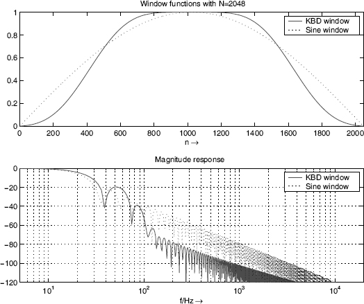
Figure 9.22 Kaiser – Bessel derived window and sine window for N = 2048 and magnitude responses of the normalized window functions.
For adjusting the time and frequency resolution to the properties of an audio signal several methods have been investigated. Signal-adaptive audio coding based on the wavelet transform can be found in [Sin93, Ern00]. Window switching can be applied for achieving a time-variant time-frequency resolution for MDCT and IMDCT applications. For stationary signals a high frequency resolution and a low time resolution are necessary. This leads to long windows with N = 2048. Coding of attacks of instruments needs a high time resolution (reduction of window length to N = 256) and thus reduces frequency resolution (reduction of number of spectral coefficients). A detailed description of switching between time-frequency resolution with the MDCT/IMDCT can be found in [Edl89, Bos97, Bos02]. Examples of switching between different window functions and windows of different length are shown in Fig. 9.24.
Temporal Noise Shaping. A further method for adapting the time-frequency resolution of a filter bank and here an MDCT/IMDCT to the signal characteristic is based on linear prediction along the spectral coefficients in the frequency domain [Her96, Her99]. This method is called temporal noise shaping (TNS) and is a weighting of the temporal envelope of the time-domain signal. Weighting the temporal envelope in this way is demonstrated in Fig. 9.25.

Figure 9.23 Normalized impulse responses of sine window for N = 2048, modulated band-pass impulse responses, and magnitude responses.

Figure 9.24 Switching of window functions.
Figure 9.25a shows a signal from a castanet attack. Making use of the discrete cosine transform (DCT, [Rao90])

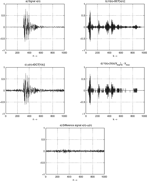
Figure 9.25 Attack of castanet and spectrum.
and the inverse discrete cosine transform (IDCT)

the spectral coefficients of the DCT of this castanet attack are represented in Fig. 9.25b. After quantization of these spectral coefficients X(k) to 4 bits (Fig. 9.25d) and IDCT of the quantized spectral coefficients, the time-domain signal in Fig. 9.25c and the difference signal in Fig. 9.25e between input and output result. One can observe in the output and difference signal that the error is spread along the entire block length. This means that before the attack of the castanet happens, the error signal of the block is perceptible. The time-domain masking, referred to as pre-masking [Zwi90], is not sufficient. Ideally, the spreading of the error signal should follow the time-domain envelope of the signal itself. From forward linear prediction in the time domain it is known that the power spectral density of the error signal after coding and decoding is weighted by the envelope of the power spectral density of the input signal [Var06]. Performing a forward linear prediction along the frequency axis in the frequency domain and quantization and coding leads to an error signal in the time domain where the temporal envelope of the error signal follows the time-domain envelope of the input signal [Her96]. To point out the temporal weighting of the error signal we consider the forward prediction in the time domain in Fig. 9.26a. For coding the input signal, x(n) is predicted by an impulse response p(n). The output of the predictor is subtracted from the input signal x(n) and delivers the signal d(n), which is then quantized to a reduced word-length. The quantized signal dQ(n) = x(n)*a(n) + e(n) is the sum of the convolution of x(n) with the impulse response a(n) and the additive quantization error e(n). The power spectral density of the coder output is SDQDQ(ejΩ) = SXX(ejΩ) ·|A(ejΩ)|2 + SEE(ejΩ). The decoding operation performs the convolution of dQ(n) with the impulse response h(n) of the inverse system to the coder. Therefore a(n)*h(n) = δ(n) must hold and thus H(ejΩ) = 1/A(ejΩ). Hereby the output signal y(n) = x(n) + e(n)*h(n) is derived with the corresponding discrete Fourier transform Y(k) = X(k) + E(k) · H(k). The power spectral density of the decoder out signal is given by SYY(ejΩ) = SXX(ejΩ) + SEE(ejΩ) · |H(ejΩ)|2. Here one can observe the spectral weighting of the quantization error with the spectral envelope of the input signal which is represented by |H(ejΩ)|. The same kind of forward prediction will now be applied in the frequency domain to the spectral coefficients X(k) = DCT[x(n)] for a block of input samples x(n) shown in Fig. 9.26b. The output of the decoder is then given by Y(k) = X(k) + E(k)*H(k) with A(k)*H(k) = δ(k). Thus, the corresponding time-domain signal is y(n) = x(n) + e(n) · h(n), where the temporal weighting of the quantization error with the temporal envelope of the input signal is clearly evident. The temporal envelope is represented by the absolute value |h(n)| of the impulse response h(n). The relation between the temporal signal envelope (absolute value of the analytical signal) and the autocorrelation function of the analytical spectrum is discussed in [Her96]. The dualities between forward linear prediction in time and frequency domain are summarized in Table 9.2. Figure 9.27 demonstrates the operations for temporal noise shaping in the coder, where the prediction is performed along the spectral coefficients. The coefficients of the forward predictor have to be transmitted to the decoder, where the inverse filtering is performed along the spectral coefficients.
The temporal weighting is finally demonstrated in Fig. 9.28, where the corresponding signals with forward prediction in the frequency domain are shown. Figure 9.28a, b shows the castanet signal x(n) and its corresponding spectral coefficients X(k) of the applied DCT. The forward prediction delivers D(k) in Fig. 9.28d and the quantized signal DQ(k) in Fig. 9.28f. After the decoder the signal Y(k) in Fig. 9.28h is reconstructed by the inverse transfer function. The IDCT of Y(k) finally results in the output signal y(n) in Fig. 9.28e. The difference signal x(n) − y(n) in Fig. 9.28g demonstrates the temporal weighting of the error signal with the temporal envelope from Fig. 9.28c. For this example, the order of the predictor is chosen as 20 [Bos97] and the prediction along the spectral coefficients X(k) is performed by the Burg method. The prediction gain for this signal in the frequency domain is Gp = 16 dB (see Fig. 9.28d).
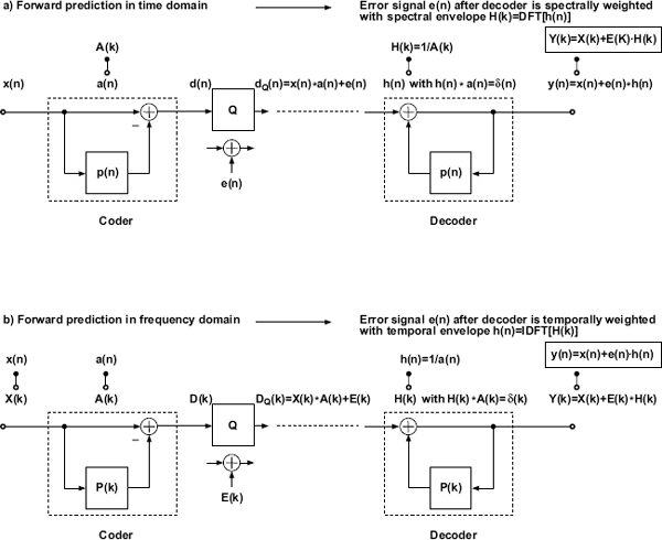
Figure 9.26 Forward prediction in time and frequency domain.

Figure 9.27 Temporal noise shaping with forward prediction in frequency domain.

Figure 9.28 Temporal noise shaping: attack of castanet and spectrum.
Table 9.2 Forward prediction in time and frequency domain.
| Prediction in time domain | Prediction in frequency domain |
| y(n) = x(n) + e(n) * h(n) | y(n) = x(n) + e(n) · h(n) |
| Y(k) = X(k) + E(k) · H(k) | Y(k) = X(k) + E(k) · H(k) |
Frequency-domain Prediction. A further compression of the band-pass signals is possible by using linear prediction. A backward prediction [Var06] of the band-pass signals is applied on the coder side (see Fig. 9.29). In using a backward prediction the predictor coefficients need not be coded and transmitted to the decoder, since the estimate of the input sample is based on the quantized signal. The decoder derives the predictor coefficients p(n) in the same way from the quantized input. A second-order predictor is sufficient, because the bandwidth of the band-pass signals is very low [Bos97].
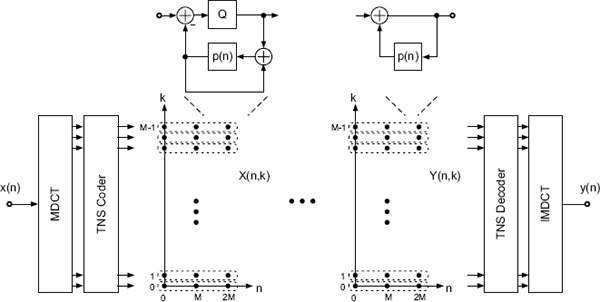
Figure 9.29 Backward prediction of band-pass signals.
Mono/Side Coding. Coding of stereo signals with left and right signals xL(n) and xR(n) can be achieved by coding a mono signal (M) xM(n) = (xL(n) + xR(n))/2 and a side (S, difference) signal xS(n) = (xL(n) − xR(n))/2 (M/S coding). Since for highly correlated left and right signals the power of the side signal is reduced, a reduction in bit rate for this signal can be achieved. The decoder can reconstruct the left signal xL(n) = xM(n) + xS(n) and the right signal xR(n) = xM(n) − xS(n), if no quantization and coding is applied to the mono and side signal. This M/S coding is carried out for MPEG-2 AAC [Bra98, Bos02] with the spectral coefficients of a stereo signal (see Fig. 9.30).
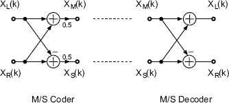
Figure 9.30 M/S coding in frequency domain.
Intensity Stereo Coding. For intensity stereo (IS) coding a mono signal xM(n) = xL(n) + xR(n) and two temporal envelopes eL(n) and eR(n) of the left and right signals are coded and transmitted. On the decoding side the left signal is reconstructed by yL(n) = xM(n) · eL(n) and the right signal by yR(n) = xM(n) · eR(n). This reconstruction is lossy. The IS coding of MPEG-2 AAC [Bra98] is performed by summation of spectral coefficients of both signals and by coding of scale factors which represent the temporal envelope of both signals (see Fig. 9.31). This type of stereo coding is only useful for higher frequency bands, since the human perception for phase shifts is non-sensitive for frequencies above 2 kHz.

Figure 9.31 Intensity stereo coding in frequency domain.
Quantization and Coding. During the last coding step the quantization and coding of the spectral coefficients takes place. The quantizers, which are used in the figures for prediction along spectral coefficients in frequency direction (Fig. 9.27) and prediction in the frequency domain along band-pass signals (Fig. 9.29), are now combined into a single quantizer per spectral coefficient. This quantizer performs nonlinear quantization similar to a floating-point quantizer of Chapter 2 such that a nearly constant signal-to-noise ratio over a wide amplitude range is achieved. This floating-point quantization with a so-called scale factor is applied to several frequency bands, in which several spectral coefficients use a common scale factor derived from an iteration loop (see Fig. 9.19). Finally, a Huffman coding of the quantized spectral coefficients is performed. An extensive presentation can be found in [Bos97, Bra98, Bos02].
9.7 MPEG-4 Audio Coding
The MPEG-4 audio coding standard consists of a family of audio and speech coding methods for different bit rates and a variety of multimedia applications [Bos02, Her02]. Besides a higher coding efficiency, new functionalities such as scalability, object-oriented representation of signals and interactive synthesis of signals at the decoder are integrated. The MPEG-4 coding standard is based on the following speech and audio coders.
- Speech coders
- – CELP: Code Excitated Linear Prediction (bit rate 4–24 kbit/s).
- – HVXC: Harmonic Vector Excitation Coding (bit rate 1.4–4 kbit/s).
- Audio coders
- – Parametric audio: representation of a signal as a sum of sinsoids, harmonic components, and residual components (bit rate 4–16 kbit/s).
- – Structured audio: synthetic signal generation at decoder (extension of the MIDI standard1) (200 bit–4 kbit/s).
- – Generalized audio: extension of MPEG-2 AAC with additional methods in the time-frequency domain. The basic structure is depicted in Fig. 9.19 (bit rate 6–64 kbit/s).
Basics of speech coders can found in [Var06]. The specified audio coders allow coding with lower bit rates (Parametric Audio and Structured Audio) and coding with higher quality at lower bit rates compared to MPEG-2 AAC.
Compared to coding methods such as MPEG-1 and MPEG-2 introduced in previous sections, the parametric audio coding is of special interest as an extension to the filter bank methods [Pur99, Edl00]. A parametric audio coder is shown in Fig. 9.32. The analysis of the audio signal leads to a decomposition into sinusoidal, harmonic and noise-like signal components and the quantization and coding of these signal components is based on psychoacoustics [Pur02a]. According to an analysis/synthesis approach [McA86, Ser89, Smi90, Geo92, Geo97, Rod97, Mar00a] shown in Fig. 9.33 the audio signal is represented in a parametric form given by

The first term describes a sum of sinusoids with time-varying amplitudes Ai(n), frequencies fi(n) and phases ψi(n). The second term consists of a noise-like component xn(n) with time-varying temporal envelope. This noise-like component xn(n) is derived by subtracting the synthesized sinusoidal components from the input signal. With the help of a further analysis step, harmonic components with a fundamental frequency and multiples of this fundamental frequency are identified and grouped into harmonic components. The extraction of deterministic and stochastic components from an audio signal can be found in

Figure 9.32 MPEG-4 parametric coder.

Figure 9.33 Parameter extraction with analysis/synthesis.
[Alt99, Hai03, Kei01, Kei02, Mar00a, Mar00b, Lag02, Lev98, Lev99, Pur02b]. In addition to the extraction of sinusoidal components, the modeling of noise-like components and transient components is of specific importance [Lev98, Lev99]. Figure 9.34 exemplifies the decomposition of an audio signal into a sum of sinusoids xs(n) and a noise-like signal xn(n). The spectrogram shown in Fig. 9.35 represents the short-time spectra of the sinusoidal components. The extraction of the sinusoids has been achieved by a modified FFT method [Mar00a] with an FFT length of N = 2048 and an analysis hop size of RA = 512.
The corresponding parametric MPEG-4 decoder is shown in Fig. 9.36 [Edl00, Mei02]. The synthesis of the three signal components can be achieved by inverse FFT and overlap-add methods or can be directly performed by time-domain methods [Rod97, Mei02]. A significant advantage of parametric audio coding is the direct access at the decoder to the three main signal components which allows effective post-processing for the generation of a variety of audio effects [Zöl02]. Effects such as time and pitch scaling, virtual sources in three-dimensional spaces and cross-synthesis of signals (karaoke) are just a few examples of interactive sound design on the decoding side.

Figure 9.34 Original signal, sum of sinusoids and noise-like signal.
9.8 Spectral Band Replication
To further reduce the bit rate an extension of MPEG-1 Layer III with the name MP3pro was introduced [Die02, Zie02]. The underlying method, called spectral band replication (SBR), performs a low-pass and high-pass decomposition of the audio signal, where the low-pass filtered part is coded by a standard coding method (e.g. MPEG-1 Layer III) and the high-pass part is represented by a spectral envelope and a difference signal [Eks02, Zie03]. Figure 9.37 shows the functional units of an SBR coder. For the analysis of the difference signal the high-pass part (HP Generator) is reconstructed from the low-pass part and compared to the actual high-pass part. The difference is coded and transmitted. For decoding (see Fig. 9.38) the decoded low-pass part of a standard decoder is used by the HP generator to reconstruct the high-pass part. The additional coded difference signal is added at the decoder. An equalizer provides the spectral envelope shaping for the high-pass part. The spectral envelope of the high-pass signal can be achieved by a filter bank and computing the RMS values of each band-pass signal [Eks02, Zie03]. The reconstruction of the high-pass part (HP Generator) can also be achieved by a filter bank and substituting the band-pass signals by using the low-pass parts [Schu96, Her98]. To code the difference signal of the high-pass part additive sinusoidal models can be applied such as the parametric methods of the MPEG-4 coding approach.
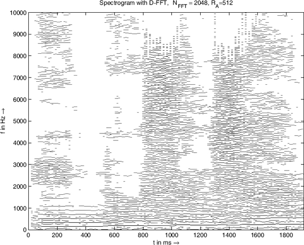
Figure 9.35 Spectrogram of sinusoidal components.

Figure 9.36 MPEG-4 parametric decoder.


Figure 9.39 shows the functional units of the SBR method in the frequency domain. First, the short-time spectrum is used to calculate the spectral envelope (Fig. 9.39a). The spectral envelope can be derived from an FFT, a filter bank, the cepstrum or by linear prediction [Zöl02]. The band-limited low-pass signal can be downsampled and coded by a standard coder which operates at a reduced sampling rate. In addition, the spectral envelope has to be coded (Fig. 9.39b). On the decoding side the reconstruction of the upper spectrum is achieved by frequency-shifting of the low-pass part or even specific low-pass parts and applying the spectral envelope onto this artificial high-pass spectrum (Fig. 9.39c). An efficient implementation of a time-varying spectral envelope computation (at the coder side) and spectral weighting of the high-pass signal (at the decoder side) with a complex-valued QMF filter bank is described in [Eks02].
9.9 Java Applet – Psychoacoustics
The applet shown in Fig. 9.40 demonstrates psychoacoustic audio masking effects [Gui05]. It is designed for a first insight into the perceptual experience of masking a sinusoidal signal with band-limited noise.
You can choose between two predefined audio files from our web server (audio1.wav or audio2.wav). These are band-limited noise signals with different frequency ranges. A sinusoidal signal is generated by the applet, and two sliders can be used to control its frequency and magnitude values.

Figure 9.39 Functional units of SBR method.

Figure 9.40 Java applet – psychoacoustics.
9.10 Exercises
1. Psychoacoustics
- Human hearing
- (a) What is the frequency range of human sound perception?
- (b) What is the frequency range of speech?
- (c) In the above specified range where is the human hearing most sensitive?
- (d) Explain how the absolute threshold of hearing has been obtained.
- Masking
- (a) What is frequency-domain masking?
- (b) What is a critical band and why is it needed for frequency masking phenomena?
- (c) Consider ai and fi to be respectively the amplitude and the frequency of a partial at index i and V(ai) to be the corresponding volume in dB. The difference between the level of the masker and the masking threshold is −10 dB. The masking curves toward lower and higher frequencies are described respectively by a left slope (27 dB/Bark) and a right slope (15 dB/Bark). Explain the main steps of frequency masking in this case and show with plots how this masking phenomena is achieved.
- (d) What are the psychoacoustic parameters used for lossy audio coding?
- (e) How can we explain the temporal masking and what is its duration after stopping the active masker?
2. Audio coding
- Explain the lossless coder and decoder.
- What is the achievable compression factor for lossless coding?
- Explain the MPEG-1 Layer III coder and decoder.
- Explain the MPEG-2 AAC coder and decoder.
- What is temporal noise shaping?
- Explain the MPEG-4 coder and decoder.
- What is the benefit of SBR?
References
[Alt99] R. Althoff, F. Keiler, U. Zölzer: Extracting Sinusoids from Harmonic Signals, Proc. DAFX-99 Workshop on Digital Audio Effects, pp. 97–100, Trondheim, 1999.
[Blo95] T. Block: Untersuchung von Verfahren zur verlustlosen Datenkompression von digitalen Audiosignalen, Studienarbeit, TU Hamburg-Harburg, 1995.
[Bos97] M. Bosi, K. Brandenburg, S. Quackenbush, L. Fielder, K. Akagiri, H. Fuchs, M. Dietz, J. Herre, G. Davidson, Y. Oikawa: ISO/IEC MPEG-2 Advanced Audio Coding, J. Audio Eng. Soc., Vol. 45, pp. 789–814, October 1997.
[Bos02] M. Bosi, R. E. Goldberg: Introduction to Digital Audio Coding and Standards, Kluwer Academic, Boston, 2002.
[Bra92] K. Brandenburg, J. Herre: Digital Audio Compression for Professional Applications, Proc. 92nd AES Convention, Preprint No. 3330, Vienna, 1992.
[Bra94] K. Brandenburg, G. Stoll: The ISO-MPEG-1 Audio: A Generic Standard for Coding of High Quality Digital Audio, J. Audio Eng. Soc., Vol. 42, pp. 780–792, October 1994.
[Bra98] K. Brandenburg: Perceptual Coding of High Quality Digital Audio, in M. Kahrs, K. Brandenburg (Ed.), Applications of Digital Signal Processing to Audio and Acoustics, Kluwer Academic, Boston, 1998.
[Cel93] C. Cellier, P. Chenes, M. Rossi: Lossless Audio Data Compression for Real-Time Applications, Proc. 95th AES Convention, Preprint No. 3780, New York, 1993.
[Cra96] P. Craven, M. Gerzon: Lossless Coding for Audio Discs, J. Audio Eng. Soc., Vol. 44, pp. 706–720, 1996.
[Cra97] P. Craven, M. Law, J. Stuart: Lossless Compression Using IIR Prediction, Proc. 102nd AES Convention, Preprint No. 4415, Munich, 1997.
[Die02] M. Dietz, L. Liljeryd, K. Kjörling, O. Kunz: Spectral Band Replication: A Novel Approach in Audio Coding, Proc. 112th AES Convention, Preprint No. 5553, Munich, 2002.
[Edl89] B. Edler: Codierung von Audiosignalen mit überlappender Transformation und adaptiven Fensterfunktionen, Frequenz, Vol. 43, pp. 252–256, 1989.
[Edl00] B. Edler, H. Purnhagen: Parametric Audio Coding, 5th International Conference on Signal Processing (ICSP 2000), Beijing, August 2000.
[Edl95] B. Edler: äquivalenz von Transformation und Teilbandzerlegung in der Quellencodierung, Dissertation, Universität Hannover, 1995.
[Eks02] P. Ekstrand: Bandwidth Extension of Audio Signals by Spectral Band Replication, Proc. 1st IEEE Benelux Workshop on Model-Based Processing and Coding of Audio (MPCA-2002), Leuven, Belgium, 2002.
[Ern00] M. Erne: Signal Adpative Audio Coding Using Wavelets and Rate Optimization, Dissertation, ETH Zurich, 2000.
[Geo92] E. B. George, M. J. T. Smith: Analysis-by-Synthesis/Overlap-Add Sinusoidal Modeling Applied to the Analysis and Synthesis of Musical Tones, J. Audio Eng. Soc., Vol. 40, pp. 497–516, June 1992.
[Geo97] E. B. George, M. J. T. Smith: Speech Analysis/Synthesis and Modification using an Analysis-by-Synthesis/Overlap-Add Sinusoidal Model, IEEE Trans. on Speech and Audio Processing, Vol. 5, No. 5, pp. 389–406, September 1997.
[Glu93] R. Gluth: Beiträge zur Beschreibung und Realisierung digitaler, nichtrekursiver Filterbänke auf der Grundlage linearer diskreter Transformationen, Dissertation, Ruhr-Universität Bochum, 1993.
[Gui05] M. Guillemard, C. Ruwwe, U. Zölzer: J-DAFx – Digital Audio Effects in Java, Proc. 8th Int. Conference on Digital Audio Effects (DAFx-05), pp. 161–166, Madrid, 2005.
[Hai03] S. Hainsworth, M. Macleod: On Sinusoidal Parameter Estimation, Proc. DAFX-03 Conference on Digital Audio Effects, London, September 2003.
[Han98] M. Hans: Optimization of Digital Audio for Internet Transmission, PhD thesis, Georgia Inst. Technol., Atlanta, 1998.
[Han01] M. Hans, R. W. Schafer: Lossless Compression of Digital Audio, IEEE Signal Processing Magazine, Vol. 18, No. 4, pp. 21–32, July 2001.
[Hel72] R. P. Hellman: Asymmetry in Masking between Noise and Tone, Perception and Psychophys., Vol. 11, pp. 241–246, 1972.
[Her96] J. Herre, J. D. Johnston: Enhancing the Performance of Perceptual Audio Coders by Using Temporal Noise Shaping (TNS), Proc. 101st AES Convention, Preprint No. 4384, Los Angeles, 1996.
[Her98] J. Herre, D. Schultz: Extending the MPEG-4 AAC Codec by Perceptual Noise Substitution, Proc. 104th AES Convention, Preprint No. 4720, Amsterdam, 1998.
[Her99] J. Herre: Temporal Noise Shaping, Quantization and Coding Methods in Perceptual Audio Coding: A Tutorial Introduction, Proc. AES 17th International Conference on High Quality Audio Coding, Florence, September 1999.
[Her02] J. Herre, B. Grill: Overview of MPEG-4 Audio and its Applications in Mobile Communications, Proc. 112th AES Convention, Preprint No. 5553, Munich, 2002.
[Huf52] D. A. Huffman: A Method for the Construction of Minimum-Redundancy Codes, Proc. of the IRE, Vol. 40, pp. 1098–1101, 1952.
[ISO92] ISO/IEC 11172-3: Coding of Moving Pictures and Associated Audio for Digital Storage Media at up to 1.5 Mbits/s – Audio Part, International Standard, 1992.
[Jay84] N. S. Jayant, P. Noll: Digital Coding of Waveforms, Prentice Hall, Englewood Cliffs, NJ, 1984.
[Joh88a] J. D. Johnston: Transform Coding of Audio Signals Using Perceptual Noise Criteria, IEEE J. Selected Areas in Communications, Vol. 6, No. 2, pp. 314–323, February 1988.
[Joh88b] J. D. Johnston: Estimation of Perceptual Entropy Using Noise Masking Criteria, Proc. ICASSP-88, pp. 2524–2527, 1988.
[Kap92] R. Kapust: A Human Ear Related Objective Measurement Technique Yields Audible Error and Error Margin, Proc. 11th Int. AES Conference – Test & Measurement, Portland, pp. 191–202, 1992.
[Kei01] F. Keiler, U. Zölzer: Extracting Sinusoids from Harmonic Signals, J. New Music Research, Special Issue: Musical Applications of Digital Signal Processing, Guest Editor: Mark Sandler, Vol. 30, No. 3, pp. 243–258, September 2001.
[Kei02] F. Keiler, S. Marchand: Survey on Extraction of Sinusoids in Stationary Sounds, Proc. DAFX-02 Conference on Digital Audio Effects, pp. 51–58, Hamburg, 2002.
[Kon94] K. Konstantinides: Fast Subband Filtering in MPEG Audio Coding, IEEE Signal Processing Letters, Vol. 1, No. 2, pp. 26–28, February 1994.
[Lag02] M. Lagrange, S. Marchand, J.-B. Rault: Sinusoidal Parameter Extraction and Component Selection in a Non Stationary Model, Proc. DAFX-02 Conference on Digital Audio Effects, pp. 59–64, Hamburg, 2002.
[Lev98] S. Levine: Audio Representations for Data Compression and Compressed Domain Processing, PhD thesis, Stanford University, 1998.
[Lev99] S. Levine, J. O. Smith: Improvements to the Switched Parametric & Transform Audio Coder, Proc. 1999 IEEE Workshop on Applications of Signal Processing to Audio and Acoustics, New Paltz, NY, October 1999.
[Lie02] T. Liebchen: Lossless Audio Coding Using Adaptive Multichannel Prediction, Proc. 113th AES Convention, Preprint No. 5680, Los Angeles, 2002.
[Mar00a] S. Marchand: Sound Models for Computer Music, PhD thesis, University of Bordeaux, October 2000.
[Mar00b] S. Marchand: Compression of Sinusoidal Modeling Parameters, Proc. DAFX-00 Conference on Digital Audio Effects, pp. 273–276, Verona, December 2000.
[Mal92] H. S. Malvar: Signal Processing with Lapped Transforms, Artech House, Boston, 1992.
[McA86] R. McAulay, T. Quatieri: Speech Transformations Based in a Sinusoidal Representation, IEEE Trans. Acoustics, Speech, Signal Processing, Vol. 34, No. 4, pp. 744–754, 1989.
[Mas85] J. Masson, Z. Picel: Flexible Design of Computationally Efficient Nearly Perfect QMF Filter Banks, Proc. ICASSP-85, pp. 541–544, 1985.
[Mei02] N. Meine, H. Purnhagen: Fast Sinusoid Synthesis For MPEG-4 HILN Parametric Audio Decoding, Proc. DAFX-02 Conference on Digital Audio Effects, pp. 239–244, Hamburg, September 2002.
[Pen93] W. B. Pennebaker, J. L. Mitchell: JPEG Still Image Data Compression Standard, Van Nostrand Reinhold, New York, 1993.
[Pri86] J. P. Princen, A. B. Bradley: Analysis/Synthesis Filter Bank Design Based on Time Domain Aliasing Cancellation, IEEE Trans. on Acoustics, Speech, and Signal Processing, Vol. 34, No. 5, pp. 1153–1161, October 1986.
[Pri87] J. P. Princen, A. W. Johnston, A. B. Bradley: Subband/Transform Coding Using Filter Bank Designs Based on Time Domain Aliasing Cancellation, Proc. ICASSP-87, pp. 2161–2164, 1987.
[Pur97] M. Purat, T. Liebchen, P. Noll: Lossless Transform Coding of Audio Signals, Proc. 102nd AES Convention, Preprint No. 4414, Munich, 1997.
[Pur99] H. Purnhagen: Advances in Parametric Audio Coding, Proc. 1999 IEEE Workshop on Applications of Signal Processing to Audio and Acoustics, New Paltz, NY, October 1999.
[Pur02a] H. Purnhagen, N. Meine, B. Edler: Sinusoidal Coding Using Loudness-Based Component Selection, Proc. ICASSP-2002, May 13–17, Orlando, FL, 2002.
[Pur02b] H. Purnhagen: Parameter Estimation and Tracking for Time-Varying Sinusoids, Proc. 1st IEEE Benelux Workshop on Model Based Processing and Coding of Audio, Leuven, Belgium, November 2002.
[Raa02] M. Raad, A. Mertins: From Lossy to Lossless Audio Coding Using SPIHT, Proc. DAFX-02 Conference on Digital Audio Effects, pp. 245–250, Hamburg, 2002.
[Rao90] K. R. Rao, P. Yip: Discrete Cosine Transform – Algorithms, Advantages, Applications, Academic Press, San Diego, 1990.
[Rob94] T. Robinson: SHORTEN: Simple Lossless and Near-Lossless Waveform Compression, Technical Report CUED/F-INFENG/TR.156, Cambridge University Engineering Department, Cambridge, December 1994.
[Rod97] X. Rodet: Musical Sound Signals Analysis/Synthesis: Sinusoidal+Residual and Elementary Waveform Models, Proceedings of the IEEE Time-Frequency and Time-Scale Workshop (TFTS-97), University of Warwick, Coventry, August 1997.
[Rot83] J. H. Rothweiler: Polyphase Quadrature Filters – A New Subband Coding Technique, Proc. ICASSP-87, pp. 1280–1283, 1983.
[Sauv90] U. Sauvagerd: Bitratenreduktion hochwertiger Musiksignale unter Verwendung von Wellendigitalfiltern, VDI-Verlag, Düsseldorf, 1990.
[Schr79] M. R. Schroeder, B. S. Atal, J. L. Hall: Optimizing Digital Speech Coders by Exploiting Masking Properties of the Human Ear, J. Acoust. Soc. Am., Vol. 66, No. 6, pp. 1647–1652, December 1979.
[Sch02] G. D. T. Schuller, Bin Yu, Dawei Huang, B. Edler: Perceptual Audio Coding Using Adaptive Pre- and Post-Filters and Lossless Compression, IEEE Trans. on Speech and Audio Processing, Vol. 10, No. 6, pp. 379–390, September 2002.
[Schu96] D. Schulz: Improving Audio Codecs by Noise Substitution, J. Audio Eng. Soc., Vol. 44, pp. 593–598, July/August 1996.
[Ser89] X. Serra: A System for Sound Analysis/Transformation/Synthesis Based on a Deterministic plus Stochastic Decomposition, PhD thesis, Stanford University, 1989.
[Sin93] D. Sinha, A. H. Tewfik: Low Bit Rate Transparent Audio Compression Using Adapted Wavelets, IEEE Trans. on Signal Processing, Vol. 41, pp. 3463–3479, 1993.
[Smi90] J. O. Smith, X. Serra: Spectral Modeling Synthesis: A Sound Analysis/Synthesis System Based on a Deterministic plus Stochastic Decomposition, Computer Music J., Vol. 14, No. 4, pp. 12–24, 1990.
[Sqa88] EBU-SQAM: Sound Quality Assessment Material, Recordings for Subjective Tests, CompactDisc, 1988.
[Ter79] E. Terhardt: Calculating Virtual Pitch, Hearing Res., Vol. 1, pp. 155–182, 1979.
[Thei88] G. Theile, G. Stoll, M. Link: Low Bit-Rate Coding of High-Quality Audio Signals, EBU Review, No. 230, pp. 158–181, August 1988.
[Vai93] P. P. Vaidyanathan: Multirate Systems and Filter Banks, Prentice Hall, Englewood Cliffs, NJ, 1993.
[Var06] P. Vary, R. Martin: Digital Speech Transmission. Enhancement, Coding and Error Concealment, John Wiley & Sons, Ltd, Chichester, 2006.
[Vet95] M. Vetterli, J. Kovacevic: Wavelets and Subband Coding, Prentice Hall, Englewood Cliffs, NJ, 1995.
[Zie02] T. Ziegler, A. Ehret, P. Ekstrand, M. Lutzky: Enhancing mp3 with SBR: Features and Capabilities of the new mp3PRO Algorithm, Proc. 112th AES Convention, Preprint No. 5560, Munich, 2002.
[Zie03] T. Ziegler, M. Dietz, K. Kjörling, A. Ehret: aacPlus-Full Bandwidth Audio Coding for Broadcast and Mobile Applications, International Signal Processing Conference, Dallas, 2003.
[Zöl02] U. Zölzer (Ed.): DAFX – Digital Audio Effects, John Wiley & Sons, Ltd, Chichester, 2002.
[Zwi82] E. Zwicker: Psychoakustik, Springer-Verlag, Berlin, 1982.
[Zwi90] E. Zwicker, H. Fastl: Psychoacoustics, Springer-Verlag, Berlin, 1990.