CONTENTS OF THIS CHAPTER

This chapter covers the following topics:

• the objectives and principles of data design;
• the design of codes;
• the scope and principles of security and control design;
• logical and physical design;
• design patterns;
• references and further reading.

DATA DESIGN

The objective of data design is to define a set of flexible data structures that will enable the realisation of the functional requirements agreed during requirements engineering, by supporting the input, output and process designs. The start point for data design is often a model of the data requirements, or a high-level business domain model, typically in the form of a UML class diagram or an entity relationship diagram. If no such analysis model is available, then the designer needs to start by producing their own model by identifying classes (or entities) from the requirements documentation (for example a requirements catalogue). One straightforward way to do this is to identify the key nouns from the narrative requirement descriptions, which become potential classes or entities. A detailed description of this process is outside the scope of this book.

Although an analysis data model is a good start point for data design, the model is typically not in a suitable format to enable a robust set of data structures to be created and, hence, requires normalising (see below). A further issue that the designer may encounter is that the analysis data model is incomplete. Additional data items (attributes), and even additional classes or entities are often required to support certain processing defined during the process design stage, or to enable future system flexibility in the form of configuration parameters.

From a normalised data model, the designer needs to agree the technology that will be used to store the data persistently. That is to say, some form of external data file(s) or even a specialist database management system (DBMS), where the data persists when the system is not running.

We shall now consider each of these aspects of data design in more detail.

Normalisation

Normalisation is a technique that designers use to derive flexible, robust and redundancy-free data structures. This means that the data structures (tables, entities or classes):

• do not contain data that can be derived;
• only contain one copy of each logical data item;
• contain the very latest value for each data item;
• accurately reflect values as per the original source from which the data was derived or that are consistent with any changes made in the system;
• combine data items into logical groups based on underlying data dependencies.

A data structure that exhibits these data qualities is said to have good data integrity.

Let us take, for example, a simple spreadsheet that is being used by a business centre for managing room bookings, as shown in Figure 9.1.

Figure 9.1 Spreadsheet showing un-normalised data

This spreadsheet highlights not only that there is redundant data in the spreadsheet (the hourly rate relates to the room that is being booked but is repeated for each booking), but that un-normalised data can become inconsistent, as is the case with the entries for training room 1 (TR1), whereby, although the same person has booked the room for Monday and Tuesday, the spelling of their name is different for each of the bookings (Dave Thomson on Monday and Dave Tomson on Tuesday). Just by looking at the data it is impossible to tell which spelling is correct. Furthermore, the hourly rate for meeting room 3 (MR3) on Monday shows as £20.00 but the same room on Tuesday shows as £25.00. Again, there is some inconsistency with the data and, again, it is not possible to determine which value is correct. We might surmise that the booking for Ben Peters in room MR1 on Monday was copied to Tuesday but MR1 was not available and, hence, the room was changed to MR3 but the user forgot to change the rate to the MR3 rate; however, it is impossible to tell from the data.

Figure 9.2 shows a set of normalised data structures derived from the un-normalised data in Figure 9.1. A detailed consideration of the process of normalisation is outside the scope of this book and interested readers are directed to some of the references listed at the end of this chapter.

Figure 9.2 Normalised data structures

As we can see from Figure 9.2, the redundant replication of the hourly rate has been removed, so that hourly rate is only recorded once, against the room. This improves the integrity of the data because, whenever the system needs to access the hourly rate, it can look it up in the Room table and always find the latest value.

Similarly, there is only one record of each booker, so that the booker’s name is only recorded once, and there is now no doubt that the correct spelling of Dave’s surname is Thomson. However, notice that, in order to normalise the data, it was necessary to invent a new unique identifier called Booker Id. This is to ensure uniqueness, because the name of the booker cannot be guaranteed to be unique. In other words, we cannot assume that there will never be another Dave Thomson who books a room in future.

Code design

In the normalisation example above, a new data item was invented to provide a unique identifier (also referred to as a key) for the Booker table. This is an example of a code. Codes are invented data items that can be used to uniquely reference certain types of data. For example, a product code is used to uniquely reference data about a particular product and a customer code is used to uniquely reference data about a particular customer.

The simplest type of code is a sequential number, as with Booker Id in Figure 9.2. If we needed to determine the data about the booker from a particular booking (for example, who booked MR3 on Tuesday at 09:00–11:00, then we can use the Booker Id value in the Booker table (1) to look up the corresponding entry in the Booking table (Ben Peters, B.A.P. Consultants).

When designing codes, the designer must consider the following criteria:

• Uniqueness. The designer must ensure that there could never be two identical values of the code relating to different data records.
• Stability. A coding system should always have the same format for all possible code values.
• Expandability. A coding system should always allow for future growth in terms of the number of unique codes that can be generated.
• Length. This is an extension of the other considerations. If a code is not long enough (for instance, not enough digits or characters), then it may not provide enough unique values to allow for future growth, and hence, the format of future codes may need to change to allow for more unique values.

There are a number of high-profile examples where code designers have not fully considered these requirements. For example, when devising a code to uniquely identify any device connected to the internet, the designers used a four-part code (Internet Protocol version 4), which provides 2³² (4,294,967,296) addresses. However, the designers did not predict the phenomenal rise in demand for mobile devices that could connect to the internet, and hence, there was a need to devise a new code, Internet Protocol version 6. IPv6 addresses are represented as eight groups of four hexadecimal digits separated by colons, which provides for 2¹²⁸, or approximately 3.4 × 1038 addresses, which is more than 7.9 × 1028 times as many as IPv4!

The Booker Id code used above is an example of using a simple sequential number. However, there are other types of code, including faceted and self-checking codes, that are worthy of further consideration.

Faceted codes

A faceted code is one that is made up of a number of parts, or facets, such as vehicle registration identification numbers, an example of which is shown in Figure 9.3, courtesy of Wikipedia.

Figure 9.3 Example of a faceted code (UK vehicle registration number)

The reason designers use faceted codes is because they are intrinsically meaningful to users of the code. In our example, system users (staff at DVLA, the Driver and Vehicle Licensing Agency) can determine the local registration office that the vehicle was registered at without needing to look it up and other relevant stakeholders may also use this system (for example, drivers may use the above registration number to determine the age of a vehicle before purchasing it). Furthermore, a faceted code can also be more robust, as separate validation can be applied to the different facets of the code.

Self-checking codes

The most common validation check performed on codes is to look up the code in some reference data table or file to determine whether it exists. If the code cannot be found then it is deemed to be invalid. However, if a code is made up of a sequential number, then it is possible for a system user to mis-type the code but still have entered a valid value. Under some circumstances, this may not be too much of a problem; for example, if the system displays back to the user some other data values associated with the code, such as the date and customer associated with a particular sequential order number. However, if we consider an online banking system, whereby a user wishes to transfer money from one account to the other, then the use of purely sequential bank account numbers could enable the transfer to go to the wrong account, which would be disastrous for the account holder making the transfer, and embarrassing for the bank. Consequently, banks use self-checking codes.

To understand how they work, let us consider the example of a bank account number as shown in Figure 9.4.

Figure 9.4 Example of a self-checking code

The main part of the account number is a sequential number, so the next available number is derived from the previously allocated number + 1. However, a sequential number alone is not robust enough so a special digit, called a check digit, is added to the end. The check digit is calculated from the sequence number using a special algorithm. This algorithm needs to ensure that, for the same source number, only one possible value can be derived for the check digit.

Once the check digit has been calculated, it is appended to the end of the source number to form the code. From here onwards, the entire code is always used, including the check digit. So when a user enters the account number, they must enter the entire code including the check digit. The computer system then strips off the check digit and recalculates it using the same algorithm, comparing the calculated value with the entered value. If the calculated check digit matches the entered check digit then the user has correctly entered the code, otherwise the system rejects the entry as invalid. If the user inadvertently switches two of the digits of the account number, when the system recalculates the check digit it will not match the check digit value entered and, hence, the system will reject the entry.

Database management systems

We have seen that data design is concerned with deriving a set of data structures to support the required inputs, outputs and processes. These structures are generally logical and independent of the target environment within which the system will be deployed. However, at some point the designer needs to decide how the data is to be stored persistently so that it is available the next time the system is executed. Traditionally, the data would be stored in a series of physical data files on a hard drive, which was perfectly adequate for single-user systems; but, with the advent of distributed, networked, multi-user systems, manipulating such files created performance difficulties and thus the new concept of the centralised database was born.

A database is a collection of organised data sets that are created, maintained and accessed using a specialist software package called a database management system (DBMS). A DBMS allows different application programs to easily access the same database. This is generally achieved by submitting a query defined using a special query language such as SQL (Structured Query Language) to the DBMS, which extracts, sorts and groups the data into a result set that is passed back to the relevant application program for further manipulation.

DBMSs may use any of a variety of database models, which define how the data is logically structured and, hence, how queries need to access the data. The most commonly-used models are: hierarchical, network, relational and object-oriented.

Hierarchical databases

With a hierarchical database, the data is organised as a set of records that form a hierarchy, as shown in Figure 9.5. In Figure 9.5, the inset diagram shows the basic structure of the database in terms of three record structures: Region, Town and Branch, where the Region record is made up of two data items (region and manager), the Town record is simply made up of the data item Town, and the Branch record is made up of three data items (branch-id, manager and no-of-staff). The main diagram shows sample data and links between the data records. The ellipsis (...) show that there is more data than can be shown on the same diagram.

Figure 9.5 Example of a hierarchical database structure

In Figure 9.5, each data node in the hierarchy has a single upward link (or parent node) and each parent node contains a number of links to its child nodes.

Hierarchical structures were widely used in the early mainframe database management systems, such as the Information Management System (IMS) by IBM, and now describe the structure of XML documents. Microsoft’s Windows® Registry is another more recent example of a hierarchical database.

Network databases

The network database model (also known as the CODASYL database model) is a more flexible derivation of a hierarchical database. Instead of each data node being linked to just one parent node, it is possible to link a node to multiple parents, thus forming a network-like structure, as shown in the example in Figure 9.6. This means that network databases can represent complex many-to-many relationships between the underlying data entities/classes, whereas hierarchical databases are restricted to simpler one-to-many structures.

Figure 9.6 Example of a network database structure

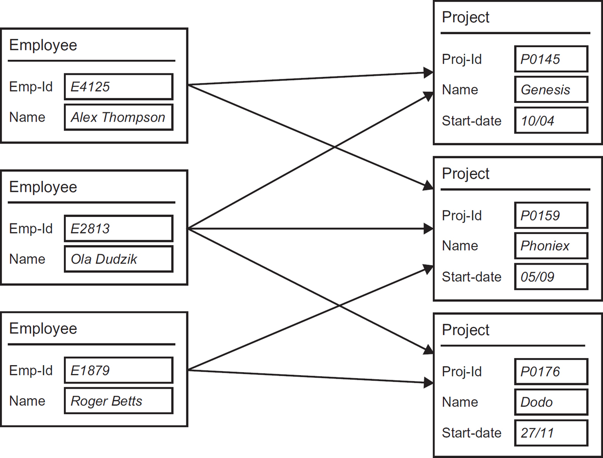
A network database consists of a collection of records connected to each other through links. A record is a collection of data items, similar to an entity in entity relationship modelling or a class in class modelling. Each data item has a name and a value. A CODASYL record may have its own internal structure and can include tables, where a table is a collection of values grouped under one data item name.

Probably the best known examples of a network DBMS are IDMS (Integrated Data Management System) and IDS (Integrated Data Store).

Relational databases

Hierarchical and network databases have largely been superseded by relational databases, based on the relational model, as introduced by E.F. Codd (Ted Codd) in 1970. This model was devised to make database management systems more independent of any particular application and, hence, more flexible for sharing databases between different applications.

The basic data structure of the relational model is the table (also referred to as a relation), where information about a particular entity is represented in rows and columns. Thus, the ‘relation’ in ‘relational database’ refers to the various tables in the database. A relation is a set of rows (referred to as tuples). The columns represent the various attributes of the entity and a row is an actual instance of the entity that is represented by the relation. Hence, in the example in Figure 9.7, which is a relational representation of the same database as Figure 9.6, there are three relations (Employee, Project and Employee-Project), Employee contains two attributes (Emp-Id and Name) and three tuples (E4125, Bob Smart; E2813, Gary Blake; E1879, Roger Betts), and so on.

Figure 9.7 Example of a relational database structure

In Figure 9.7, the relationships between the Employee and Project relations (as identified in Figure 9.6 as links between the records) have been represented in a separate table, which contains Emp-Id and Proj-Id as its columns. These columns show a * beside the column names, which identifies them as foreign keys. Relationships between tuples in different tables in a relational database are maintained by copying the primary key (one or more columns whose values can uniquely identify each tuple in a relation) from one table into another, where it becomes a foreign key. These foreign key values can be used to join the table to the original table, where the primary key values match the foreign key values. When accessing the data in a relational database, a query is issued to the DBMS, which then joins the necessary tables together, and if the query requires it, filtering and sorting the resultant table, which becomes the result set that is passed back to the query’s originator (typically a program). Figure 9.8 shows the result set produced by joining the relations in Figure 9.7.

Figure 9.8 Example of a result set from joining relations

One of the strengths of the relational model is that, in principle, any value occurring in two different records (belonging to the same table or to different tables), implies a relationship among those two records. In other words, relationships between tables are established by the fact that the tables share common attributes.

There are a number of examples of relational database management systems (RDBMS) in general use, but perhaps the most common are Oracle (from Oracle Corporation®), SQL Server (from Microsoft®) and DB2 (from IBM®).

Object-oriented

Many OO applications, whilst manipulating objects at run-time, need to hold a persistent copy of the data that is encapsulated within the objects, in some form of permanent store. Consequently, there is often a need to store the data in a database and then load it into a set of objects at run-time, saving the data back to the database before the application shuts down. Hence, many OO systems use relational databases to store their data persistently, a technique referred to as object-relational mapping.

Object-oriented database management systems (OODBMS) started to evolve from research in the early to mid 1970s, with the first commercial products appearing around 1985. These new database technologies enabled OO developers to retain the objects that they manipulated at run-time, reducing the need for object-relational mapping. However, perhaps more importantly, they introduced the key ideas of object programming, such as encapsulation and polymorphism, into the world of databases.

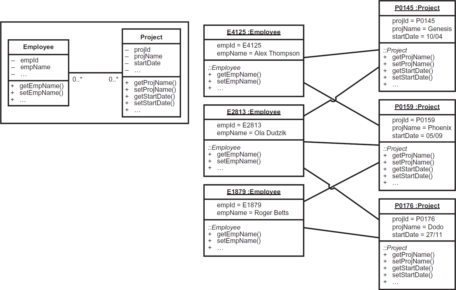
OO databases store data as a series of objects that are connected to each other by pointers. This means that the actual data can be directly accessed only through the invocation of one of the object’s operations, which can then build in security and integrity rules to ensure that the data cannot be corrupted or accessed by unauthorised users. This is highlighted in Figure 9.9, which shows an OODB structure, by the use of visibility adornments against the attributes and operations. These same adornments were shown in the class diagram extract in Figure 8.16, but Figure 9.9 shows objects (instances of classes) rather than classes. (Note: the class diagram defining the structure for the objects and how they are associated is shown in the inset in Figure 9.9.)

In Figure 9.9, the objects are stored so that they can only be manipulated by their public operations; their attributes are shown as private. There are two main differences between object diagrams and class diagrams: first, the top compartment of the object box contains the identifier of the object as a prefix to the name of the class to which it belongs; and second, the attributes also include the values that relate to each object.

One common use of OODBMS technology is within environments that dynamically manage a large set of ‘live’ objects within limited memory resources, such as application servers. Objects are temporarily persisted into a local OODBMS, from which they can be quickly recovered when required.

Figure 9.9 Example of an object database structure

Physical files

Although DBMSs are the most popular way to store data persistently because they create an interface between the application programs and the physical stored data, effectively de-coupling the data from the applications that manipulate it, they are not the only option. Some systems require that they directly manipulate data files stored on disk. This makes the system’s designer’s and developer’s job more complex, but enables the use of proprietary data structures that are tailored to the specific needs of the application.

When designing data file structures, two fundamental factors must be considered:

1. how to physically organise the data on a disk (disk being the most utilised of permanent storage media);
2. how to access/retrieve the stored data.

File organisations

The two most common data file organisations are serial and sequential.

With serial files, the records contained in the file are physically organised in the order in which they are created (in other words, in no logical sequence), as in Figure 9.10, which shows a simple file of employee records, with only two data items (known as fields); the first containing the employee Id and the second the employee name.

Figure 9.10 Example of a serial file organisation

In Figure 9.10 none of the data fields are in any particular order. This organisation, whilst being more difficult to gain access to the data (as discussed later), is simple to add to. This is because, when a new record needs to be added to the file it is simply appended to the end of the file, requiring no re-organisation. However, if an application program needs to access the data in any sequence other than the sequence in which the records were created (for instance in Surname, Firstname or Emp-id sequence), then the program would need to start retrieving the data with the first record and then keep skipping through the records until the required data had been found. This is generally a very time-consuming task, especially if there is a large number of records in the file, and/or each record is quite large, in terms of the number and size of the data items recorded.

An alternative to the serial file is the sequential file. As the name implies, with a sequential file, the data records are physically stored on disk in some particular sequence (such as Emp-id sequence, as per Figure 9.11).

Like the serial file, the sequential organisation has both advantages and disadvantages. On the positive side, records in a sequential file are much easier to access/retrieve. This is because the application knows the sequence and can therefore perform some form of search algorithm to help reduce the time that would have been spent skipping through each record one at a time, if the file were serial. A relatively simple algorithm is the binary chop, whereby the program continually narrows down the scope of records to check on the negative side; adding new records to a sequential file necessitates a complete re-organisation of the file each time, which can be extremely time-consuming.

Figure 9.11 Example of a sequential file organisation

File access/retrieval mechanisms

We have already considered the issues with accessing data from a serial file, and the fact that it is much quicker to retrieve data from a sequential file. Consequently, the most popular approach to manipulating data in physical files is to store the actual data in a serial file, whilst using a sequential file as an index into the serial file, as shown in Figure 9.12.

Figure 9.12 Example of an index file

The concept of an index file is essentially the same as using an index in a book. To find the entry that you are looking for, you first look it up in the index to find the corresponding page number, and then you can skip quickly to the required page. The same is true when accessing data using an index file.

The index file is a sequential file where the records are physically organised in the order of the key values. The key represents the value that is being sought (in the case of Figure 9.12, the key contains Emp-Id values). Consequently, the index file can be quickly scanned using an algorithm such as the binary chop, mentioned above, so that a pointer to the actual data record can be obtained. For example, if the index file in Figure 9.12 is scanned for the key value E2531, then this would result in a pointer to record number 8 in the serial data file.

Although indexed files tend to be the most common, some applications use a more specialist form of file retrieval whereby the actual location of the required data on the disk (known as the disk address), can be derived by applying a special algorithm to the key value. These files are collectively referred to as direct files.

SECURITY AND CONTROL DESIGN

System controls are mechanisms used by the designer to ensure the integrity of the system from both a data and process perspective. There are several reasons why this is important, including:

• to comply with legislation or industry regulations (for example, data protection legislation requires that any data relating to individuals is protected from unauthorised access, and is correct and up to date);
• to enforce business rules and policies (for example, an organisation may have a rule that all purchase invoices must undergo an authorisation process before they can be paid);
• to protect an organisation’s intellectual property and commercial interests (for example, access to an organisation’s customer database and sales data may enable a competitor to poach customers by undercutting their prices);
• to ensure the accuracy of any data used to inform management decision-making (for example, (1) an organisation’s senior management may decide to invest in a product based on previous sales figures, which, if they are incorrect may lead to heavy losses, or (2) inaccurate data about a customer’s order may lead to dissatisfaction and loss of business).

The designer may devise a range of different controls aimed at complying with rules and regulations and ensuring system integrity. Some system controls are designed to prevent user errors during data input and the execution of system processes, whilst others prevent the unauthorised use of the computer system or unauthorised access to data.

Systems controls can broadly be categorised as:

• input and output controls;
• data controls;
• process controls;
• security and audit.

In practice, there are significant overlaps between each area.

Input controls

Input controls are devised by the designer during I/O design to ensure and enforce the accuracy of data input into the system.

Input controls fall into two categories: verification and validation, which have already been briefly discussed but are expanded upon below. A further set of controls, referred to as clerical controls, may also be devised to ensure that any manual data entry activities are robust.

Whilst we have classified verification and validation as input controls, the likelihood is that they will actually be enforced within the processes that sit behind the data entry forms. Furthermore, some of the validation rules may well be implemented as part of the physical data design, as constraints within a database schema definition.

Verification of input data

One of the biggest issues facing the designer when designing input mechanisms, particularly those that rely on keyboard data entry, is that of detecting and preventing transcription errors. In the context of keyboard data entry, this is where the user inadvertently transcribes (changes the order of) the characters being entered. The process that the designer implements in order to detect or prevent transcription errors is called verification and the most popular techniques used are:

• Double-keying. The user is asked to type the same data field twice and the two entries are compared. If the entries do not match, then one has been input incorrectly and the user is asked to re-key. This is used for critical entries such as email addresses (where email is the main source of communication with the data subject) and when creating new passwords.
• Self-checking codes. Covered earlier in this chapter, check digits are used for critical codes such as account numbers where, if the user types the entry incorrectly, the result may still be a valid code and cause critical integrity issues.
• Repeating back what the user entered. Data entered is displayed back to the user (or for voice-recognition inputs, the spoken inputs are converted into audio outputs) for confirmation by the user.

Validation of input data

• Existence checks. The most effective way to check the accuracy and validity of a piece of data is to check if the value exists in some kind of reference file. However, this only works for certain kinds of pre-defined data, such as product codes and customer account numbers, where there is a set of pre-defined values held in a reference file.
• Range checks. For certain types of data, it is possible to check that the data value falls within a range of valid values. For example, the month part of a date must between 1 and 12.
• Cross-field validation. Often there are relationships between different items of data. For example, in a sales order processing system, the date an order is despatched cannot be prior to the date the order was placed.

Output controls

Output controls are devised by the designer to ensure that the output from the system is complete and accurate and that it gets to the correct intended recipients in a timely manner.

Output controls include:

• Control totals. Used to check whether the right number of outputs have been produced and detect whether, for example, some outputs have gone missing or have not been produced. Furthermore, where outputs take the form of data files for transfer to another system, it is common practice to include special header and/or footer records containing control totals so that as the receiving system processes the file, it calculates the totals and compares the calculated totals against the values stored in the header and/or footer record(s). If the two do not match, then the file has either become corrupted or a problem has occurred when reading or processing the data.
• Spot checks. Used where output volumes are very large and it is not feasible to check every item produced. For example, spot checks could be conducted on a sample of payslips produced by a payroll bureau, to ensure that the correct amounts have been calculated for the correct employees. Spot checks can also be conducted for abnormally high values, as identified using an exception report. For example, checking any payslip where the amount paid exceeds £10,000 in any one month.
• Pre-numbering. Some outputs are produced on special pre-numbered stationery, such as invoices or cheques. Clerical controls could be put in place to ensure that there are no gaps in sequence numbers, or that where there are gaps, they are accounted for (for example, documents that were spoiled during printing).

Clerical controls

Clerical controls can be used for both inputs and outputs and are essentially processes that are implemented and carried out manually to eliminate user errors and loss or corruption of the source data prior to data entry, or after the production of a system output. These kinds of control are particularly common in accounting systems where the accuracy of data is paramount.

A common form of clerical control is the use of some form of batch control document. When a batch of input source documents is received at a data processing centre, a member of staff prepares the batch for keying by a data entry operator. This preparation usually involves physically collating the documents together and completing the batch control document, which typically contains the following information:

• Serial number of the batch. To enable checking to determine whether the batch follows the previous batch received. This can help identify if an entire batch has gone missing.
• Count of batch contents. The number of forms that should be in the batch. This can be checked against the number of forms keyed by the data entry operator and can identify if one or more forms within the batch go missing.
• Serial numbers of forms in the batch. The serial numbers or number range(s) of the enclosed forms. Again, this may identify if forms within the batch go missing.
• Batch control totals. One or more values on each form can be added together to provide an overall total for the batch. For example, a common control total for a batch of purchase invoices is the total value of all of the invoices added together. This can help identify if any of the documents have been mis-keyed.
• Hash totals. A form of batch control, but instead of producing a meaningful total, such as total invoice value in the batch, a meaningless value is produced by totalling a field such as the invoice number.

Clerical controls are particularly important where source documents are posted – either from location to location or via the internal post within a specific site – as it is very easy for documents to be lost in transit, with the result that certain transactions do not take place.

Data controls

We have already considered certain data controls in terms of validation, discussed under I/O controls. Validation rules are typically applied at individual data item level, or across two data items, in the case of cross-field validation. For example, an order date cannot be blank and cannot be later than the delivery date. Further rules relating to each data item are often defined by the analyst, but some may need to be specified by the designer during data design, typically in a document called a data dictionary, or within the repository of a software-based modelling tool. The data dictionary would define the following information about each data item, which effectively imposes constraints on the data items that must be enforced by system controls and tested during systems testing:

• Data type. During system development, when databases/data files are created, and during programming, each data item that is created must be assigned a data type. The data type determines which data values can be stored in the data item. Some data types are generic (such as alphanumeric, character, numeric, date, logical) whilst others are specific (native) to a particular DBMS or programming language.
• Length. The length of the data item is also specified, which, again, constrains the valid values that the data item can hold.
• Format. Some data items may also have additional constraints imposed upon them in terms of the format that valid values may take. For example, the Emp-Id data item in Figures 9.6 to 9.12 would have a data type of alphanumeric (meaning that it can contain a mix of alphabetic and numeric characters), a length of four, and the first character must be alphabetic; the remaining three characters must be numeric.
• Value range. Some data items may be further constrained by specifying that valid data values must fall within a specific range. For example, the Emp-Id data item may be constrained so that it may only take on values between E1000 and E5000.
• Mandatory. Identifies whether the data item must contain a value or can be left blank/empty. This is generally checked during data entry as part of the validation of input data, but can also be checked by a DBMS when new data is added to the database.
• Default value. Some data items may be defined with a default value(s) – a value that will automatically appear in the data item when the data is input or added to a database.
• Visibility. In some data dictionaries – for example, those defined using a UML modelling tool – it is also possible to define the visibility of each data item. This then constrains how the data item can be used, as further controls can be built into the definitions of operations that are used to access the data. As we saw earlier, the attributes of an object can be specified in a UML class definition as being private (their visibility is set to private), which means that the data cannot be accessed directly and, hence, can only be accessed via the object’s operations. Figure 8.16 shows a class with private attributes and public operations.

In addition to these field-level data controls, additional controls can be derived from the logical data model (entity relationship diagram or class diagram), produced during data design. The data model defines some of the business rules of the organisation, and so, by default, determines some of the controls that must be implemented and tested. For example, the class model in Figure 8.17 states that a Medical can be associated with one (and only one) Life policy but a Life policy can exist without a corresponding Medical. Such rules preserve the integrity of the data as well as forming the basis for subsequent systems testing.

Code design can assist in data control. It may be feasible to implement a code design which has elements of self checking. Thus the first facet of the code (say the first three numbers) may be split off and certain checks performed. This might include consistency checks against other parts of the code.

Process controls

We have already discussed the fact that system controls are devised to enforce business rules, which can be defined within a data model. However, there are other models produced both during systems analysis and systems design. For example, many systems enforce some form of process workflow, which can be explicitly captured in some form of state model, such as a UML state machine diagram or a state transition diagram.

Figure 9.13 shows a UML state machine diagram that represents the states that a purchase invoice object can pass through within its life.

Figure 9.13 UML state machine diagram showing the lifecycle for an invoice object

Figure 9.13 clearly shows that, once an invoice has been received, it can either be authorised or rejected, and, more importantly, only authorised invoices can be paid (as there is no transition between the states Rejected and Paid. This rule would be implemented using a system control built into the Pay Invoice process, by checking the status of the invoice object to ensure that it is Authorised and, if not, cancelling the payment process.

Security and audit

Security is a special kind of system control that is devised to prevent unauthorised access to the system or to certain functions or data held within the system, and prevent loss of, or corruption to, system artefacts as a result of a range of risks including fire, flood, terrorist attack and Acts of God.

In terms of security, the options available to the designer can be broadly categorised as physical or logical security. However, there is a further aspect to security design that is not about the prevention of access or loss of system artefacts, but concerns the traceability of user activity: systems audit.

Apart from the fact that organisations hold sensitive data relating to their operations, which could be used to their detriment by their competitors, there are also legal imperatives in having a robust security design, in the form of data protection and computer misuse legislation.

Physical security

Physical security measures prevent direct access to computer equipment, including workstations, servers and backing storage. The most common mechanisms used are:

• Locks. Including key-based locks, combination locks and swipe card activated locks. Also, biometric options are becoming more commonplace, including fingerprint and retina recognition to activate the lock.
• Barriers. Similar to locks, but where a barrier of some kind blocks the entry into a building containing computer equipment. Again, these can be activated either using swipe cards, combination codes or biometrics, or a combination of these mechanisms.
• Safes. Safes are often used as part of a backup and recovery policy (see below) to provide physical protection to computer media (like CDs, DVDs, magnetic tape, microfiche) from theft or damage/destruction by a range of risks identified above.
• Security personnel. Often combined with the use of barriers to check that any personnel attempting to gain access to a building have the appropriate authorisation to do so.
• Backup and recovery. There are a variety of measures that can be taken to ensure that copies of the system artefacts, including hardware, software components and data, are available to enable the system to be recovered/restored following loss as a result of the risks identified above. Considerations of the various options available are outside the scope of this book.

Logical security

Logical security measures involve aspects of the software that make up the system in order to protect the system and its data from unauthorised access, destruction or corruption. The most common mechanisms are:

• Access controls. The most common form of logical access controls are passwords and PINs (Personal Identification Numbers), which must be correctly entered via a computer keyboard or keypad. These are often combined with physical security mechanisms in a multi-stage process that includes identification, authentication and authorisation:
  1. Identification – the user enters a user name to identify themselves.
  2. Authentication – the system checks that the user is who they say they are, often using a ‘three-factor’ approach which comprises:
     1. Something they know (such as a password or PIN).
     2. Something they have (such as a card or key).
     3. Something they are (such as a fingerprint or other biometric).
  3. Authorisation – the system checks what level of access (permissions) the user has been granted, both individually and as a member of one or more groups.
• Firewalls. Firewalls are special software locks that filter incoming access to a computer network to ensure that the access originates from a trusted or authorised source. Firewalls are used in addition to other logical and physical security mechanisms because traditional security mechanisms are not sufficient in a world where more and more computers and systems are connected to one another via the internet and by wide area networks, and hackers can gain remote access to systems almost undetected.
• Encryption. Encryption provides an additional level of security, above and beyond the traditional logical and physical mechanisms, to ensure that any data being transmitted from one system to another cannot be read, even if it is intercepted by an unauthorised party. Only the intended recipient of the data can read it using a special ‘encryption key’ to de-crypt the encrypted data. As well as being used to protect data in transit, encryption is also used to protect data stored in databases or local hard drives, so that only authorised users can read the data.
• Anti-malware software. The advent of open systems and the internet has increased the risk of systems being targeted by malware (malicious software), such as viruses, trojans, worms, spyware to name but a few. This specialist software is used to detect such malware and eradicate it before it can corrupt any software artefacts or data.

System audit trail

Audit trails are implemented to maintain traceability of activities that take place within a system. An audit trail logs system activity in terms of who did what, when and on which piece of equipment. They are commonly used for four different purposes:

• To check the integrity of the system data by tracing through transactions that have taken place. This is often a requirement of annual audit reviews by internal and external auditors.
• To provide a record of compliance. For example, UK data protection legislation requires that personal data (data relating to individuals) is obtained fairly and lawfully. Consequently, systems often include a tick box for the data subject to indicate their approval for the data to be used in a certain way. A record of this permission is then logged in the audit trail to provide evidence of compliance with that requirement.
• To detect and recover from failed system transactions in order to maintain data integrity, for example a payment without a corresponding invoice. It may be possible to find the original transaction and re-apply it to correct the data.
• To identify any unauthorised or fraudulent activity that has taken place within the system.

Although audit information will vary from system to system, most audit records include the following information:

• unique sequence number;
• date of the transaction;
• time of the transaction;
• user ID of the person making the transaction;
• machine ID of the device used to make the transaction;
• type of transaction (such as Payment, Credit Note, Invoice, and so on);
• transaction value(s);
• data value(s) before transaction;
• data value(s) after transaction.

Sometimes auditors use specialised audit review tools, and hence the designer may need to ensure that the audit trail is maintained in a format compatible with such tools.

LOGICAL AND PHYSICAL DESIGN

Design activities can be divided into two separate stages of design: logical design and physical design. The former is ‘platform-agnostic’ insofar as it makes no specific reference to the implementation environment or technologies, and the latter defines how the logical solution elements (inputs, outputs, processes and data) are to be built and deployed using specific technologies and infrastructure of the target implementation environment.

Although some designers may not perform a separate logical design stage, jumping straight to environment-specific implementation specifications, a common approach is to start with a platform-agnostic solution design that is then ‘tuned’ to take advantage of the specifics of a particular technological implementation environment. A benefit of splitting design into these two separate stages is that a generic solution can be proposed that can be adapted for implementation in a range of different environments. This is how the design objective of portability is achieved.

Much of this chapter has been about logical design, but there are areas that relate to specific technologies. I/O design in particular is difficult to achieve without making reference to specific technologies because use of particular technologies is an integral design consideration in order to achieve the I/O requirements of a system.

We shall now briefly consider some of the issues facing the designer when undertaking physical data design and physical process design.

Physical data design

Physical data design involves taking the normalised data model produced during logical data design and ‘tuning’ it for implementation using specific data storage technologies and media. We have already considered some of the options available to the designer in terms of DBMSs and physical file structures. During this logical-to-physical mapping exercise, it is common to ‘de-normalise’ the logical data model in order to improve system performance. De-normalisation re-introduces data redundancy that was removed during the normalisation process (as described earlier in this chapter).

Physical process design

We have already considered approaches to logical process design and specification, in particular, identification and definition of logical software components. Physical process design then considers which technologies to use in order to build the components and how they should be deployed within the implementation environment. Figure 9.14 shows an example of a UML deployment diagram that can be used to specify how physical components are to be deployed.

In Figure 9.14, each component has been stereotyped with the technology used to build/deploy it, such as ≪iPad app≫ and ≪java servlet≫. Furthermore, the diagram shows the physical devices (referred to as nodes in UML), denoted by the three-dimensional cubes, where each component will be deployed in the target implementation environment. Also note that some of the nodes are referred to as ≪execution environment≫. These represent special software environments such as the Oracle 11i DBMS, web browser and web server.

Figure 9.14 UML deployment diagram showing physical components

DESIGN PATTERNS

Designers are often faced with similar challenges to those that they have already solved in the past. Rather than ‘re-inventing the wheel’, they go back to a previous design with similar challenges to the one they currently face and use that as a template (pattern) for their current design. This approach has continued in an informal way for many years, but became more formalised with the advent of the seminal book Design patterns: Elements of reusable object-oriented software by Erich Gamma and others (1994).

In general, formally defined patterns have four essential elements:

• Pattern name – a handle for describing the design problem.
• Problem – this describes when to apply the pattern by explaining the problem and its context.
• Solution – this describes the elements that make up the design, their relationships, responsibilities and collaborations. The solution is a template, an abstract description of a design problem and how a general arrangement of elements can be used to solve it.
• Consequences – are the results and trade-offs of applying the pattern and help the designer to understand the benefits and disadvantages of applying the pattern.

The Gamma book introduced a set of template solutions to address common design problems. Each pattern is named, leading to the adoption of a common vocabulary for designers, who can simply refer to the names of design patterns rather than having to explain them to their peers. This has also led to a more standardised approach to systems design across the IT industry.

Gamma and his co-writers acknowledge that their book only captures a fraction of what an expert might know. It does not have any patterns dealing with concurrency, distributed programming or real-time programming. It does not include any application domain-specific patterns. However, since the publication of the book, the concept of patterns has been extended to other IT disciplines and now architectural patterns and analysis patterns are commonplace.

Design patterns make it easier to reuse successful designs and architectures. The patterns presented by Gamma et al. are independent of programming language and hence can be adopted during logical design and tuned during physical design. Most of the patterns are concerned with achieving the design objectives of minimising coupling and maximising cohesion, introduced earlier in this chapter. They achieve this through abstraction, composition and delegation, in turn fundamental principles of OO design.

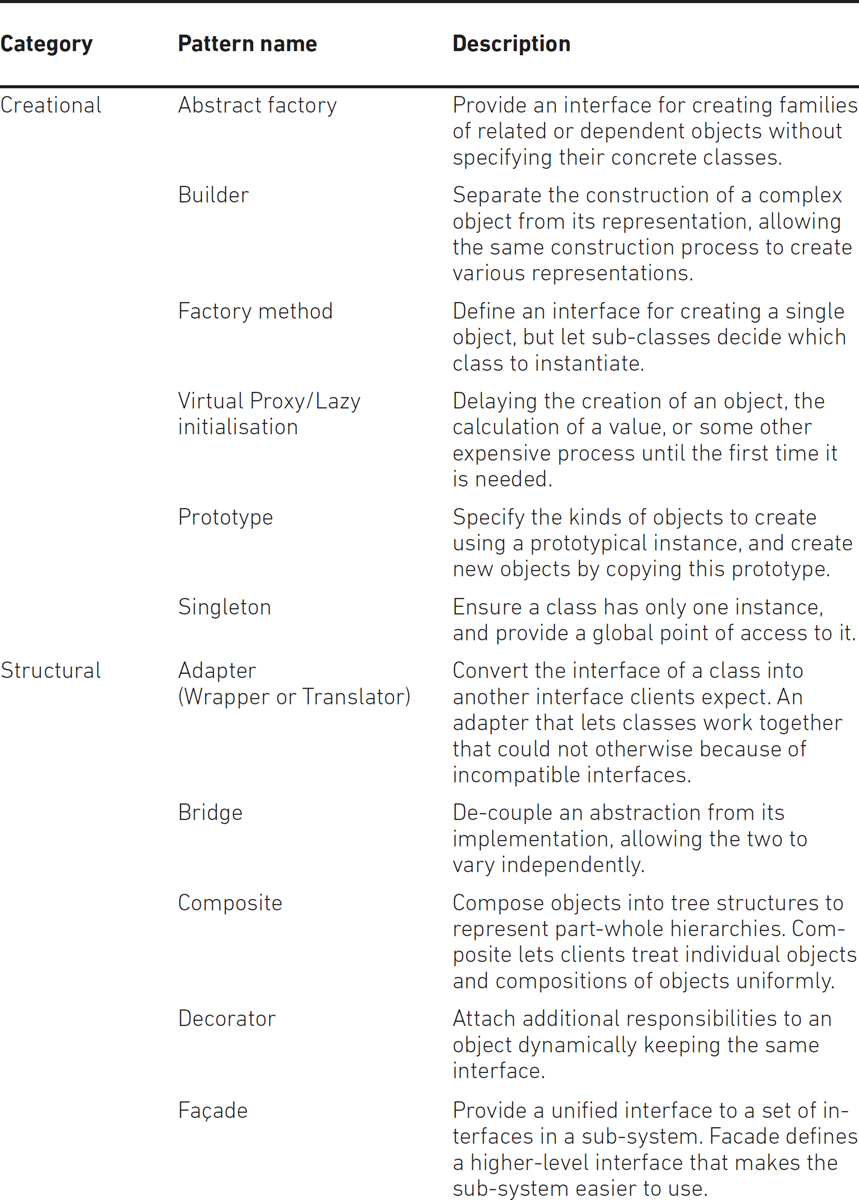
Design patterns were originally grouped into three categories: creational patterns, structural patterns and behavioural patterns. However, a further classification has also introduced the notion of architectural design pattern, which may be applied at the architecture level of the software, such as the Model–View–Controller pattern. Table 9.1 provides a summary of the most commonly-used design patterns, although a detailed explanation of each pattern is beyond the scope of this book.

Table 9.1 Common design patterns (after Gamma et al.)

REFERENCES

Gamma, E., Helm, R., Johnson, R. and Vlissides, J. (1994) Design patterns: elements of Reusable Object-Oriented Software. Addison-Wesley, Boston, MA.

FURTHER READING

Arlow, J. and Neustadt, I. (2005) UML2 and the unified process: practical object-oriented analysis and design (2nd edition). Addison-Wesley, Boston, MA.

Codd, E. F. (1990) The relational model for database management, version 2. Addison-Wesley, Boston, MA.

Date, C. J. (2004) An introduction to database systems (8th edition). Addison-Wesley, Boston, MA.

Pressman, R. S. (2010) Software engineering: a practitioner’s approach (7th edition). McGraw-Hill, New York.

Rumbaugh, J., Jacobson, I. and Booch, G. (2005) The Unified Modeling Language reference manual (2nd edition). Addison-Wesley, Boston, MA.

Skidmore, S. and Eva, M. (2004) Introducing systems development. Palgrave-MacMillan, Basingstoke.

Yeates, D. and Wakefield, T. (2003) Systems analysis and design (2nd edition). FT Prentice Hall, Harlow.