6. More Tools and Techniques for Evaluating Regression Models

Overview

This chapter explains how to evaluate various regression models using common measures of accuracy. You will learn how to calculate the
Mean Absolute Error (MAE) and Root Mean Squared Error (RMSE), which are common measures of the accuracy of a regression model. Later, you will use Recursive Feature Elimination (RFE) to perform feature selection for linear models. You will use these models together to predict how spending habits in customers change with age and find out which model outperforms the rest. By the end of the chapter, you will learn to compare the accuracy of different tree-based regression models, such as regression trees and random forest regression, and select the regression model that best suits your use case.

Introduction

You are working in a marketing company that takes projects from various clients. Your team has been given a project where you have to predict the percentage of conversions for a Black Friday sale that the team is going to plan. The percentage of conversion as per the client refers to the number of people who actually buy products vis-à-vis the number of people who initially signed up for updates regarding the sale by visiting the website. Your first instinct is to go for a regression model for predicting the percentage conversion. However, you have millions of rows of data with hundreds of columns. In scenarios like these, it's very common to encounter issues of multi-collinearity where two or more features effectively convey the same information. This can then end up affecting the robustness of the model. This is where solutions such as Recursive Feature Selection (RFE) can be of help.

In the previous chapter, you learned how to prepare data for regression modeling. You also learned how to apply linear regression to data and interpret the results.

In this chapter, you will learn how to evaluate a regression model to judge its performance. Specifically, you will target metrics such as the Mean Absolute Error (MAE) and Root Mean Squared Error (RMSE).

You will build on this knowledge by learning how to evaluate a model. Learning this skill will help you choose the right features to use for a model, as well as to compare different models based on their MAE and RMSE values. Later on in the chapter, you will learn about RFE, which is a powerful and commonly used technique for selecting only the most relevant features for building a regression model, thereby removing the redundant ones. Finally, you will learn about tree-based regression methods, and why they sometimes outperform linear regression techniques.

Let's begin this chapter by learning how to evaluate the accuracy of a regression model.

Evaluating the Accuracy of a Regression Model

To evaluate regression models, you first need to define some metrics. The common metrics used to evaluate regression models rely on the concepts of residuals and errors, which are quantifications of how much a model incorrectly predicts a particular data point. In the following sections, you will first learn about residuals and errors. You will then learn about two evaluation metrics, the MAE and RMSE, and how they are used to evaluate regression models.

Residuals and Errors

An important concept in understanding how to evaluate regression models is the residual. The residual refers to the difference between the value predicted by the model and the true value for a data point. It can be thought of as by how much your model missed a particular value. In the following diagram, we can see a best-fit (or regression) line with data points scattered above and below it. The distance between a data point and the line signifies how far away the prediction (xi,yi) is from the actual value (xj,yj). This difference is known as a residual. The data points below the line will take negative values, while the ones above will take positive values:

Figure 6.1: Estimating the residual

The residual is taken to be an estimate of the error of a model, where the error is the difference between the true process underlying the data generation and the model or, in other words, the difference between the actual value and the predicted value. We cannot directly observe the error because we do not know the true process, and therefore, we use the residual values as our best guess at the error. For this reason, error and residual are closely related and are often used interchangeably. For example, if you were asked to build a machine learning model for predicting the average age of all the people in a country, the error would mean the difference between the actual average age and the predicted average age. However, finding the actual average would be a difficult task as you would need to collect data for the whole country. Still, you could make the best guess at the average by taking the mean of the ages of some of the people in the country. This guess can then be used to find the residual, and hence serve as the error.

At this point, you might be thinking, why do we need any other evaluation metric? Why not just take the average of residuals? Let's try to understand this with the help of an example. The following table presents the actual selling price of some items and the selling prices for the same items predicted by a machine learning model (all prices are in Indian National Rupee):

Figure 6.2: Average residual calculation

As you can observe in Figure 6.2, the average residual is zero; however, notice that the model is not performing well. It is missing every data point. Therefore, we know for sure that the error is non-zero. The reason we are getting the average residual as zero is that the negative and positive values of residuals are canceling out, and therefore we must go for absolute or squared values of residuals. This helps in focusing only on the magnitude of residuals.

Let's discuss two of the most commonly used evaluation metrics – the MAE and RMSE, both of which follow the reasoning we discussed in the earlier paragraph. Instead of focusing on the positive or negative signs of the residuals, both the MAE and RMSE convert the residuals into magnitudes, which gives the correct estimate of the model's performance.

Mean Absolute Error

There are multiple ways to use residuals to evaluate a model. One way is to simply take the absolute value of all residuals and calculate the average. This is called the Mean Absolute Error (MAE), and can intuitively be thought of as the average difference you should expect between your model's predictions and the true value:

Figure 6.3: Equation for calculating the MAE of a model

In the preceding equation, yj is the true value of the outcome variable for the data point j, and ŷj is the prediction of the model for that data point. By subtracting these terms and taking the absolute value, we get the residual. n is the number of data points, and thus by summing over all data points and dividing by n, we get the mean of the absolute error.

Therefore, a value of zero would mean that your model predicts everything perfectly, and larger values mean a less accurate model. If we have multiple models, we can look at the MAE and prefer the model with the lower value.

We can implement MAE using the scikit-learn library, as shown here:

1. We will import the mean_absolute_error metric from the sklearn.metrics module:

   from sklearn.metrics import mean_absolute_error

2. Next, we just need to call the mean_absolute_error function with two arguments – predictions, and the ground_truth values:

   MAE = mean_absolute_error(predictions, ground_truth)

One issue with the MAE is that it accounts for all errors equally. For many real-world applications, small errors are acceptable and expected, whereas large errors could lead to larger issues. However, with MAE, two medium-sized errors could add up and outweigh one large error. This means that the MAE may prefer a model that is fairly accurate for most predictions but is occasionally extremely inaccurate over a model with more consistent errors over all predictions. For this reason, instead of using the absolute error, a common technique is to use the squared error.

Root Mean Squared Error

As we discussed earlier, another way of focusing only on the magnitudes of residuals is by squaring their values, which helps in getting rid of the positive or negative signs. This concept serves as the core of the RMSE metric. Before we jump into the details of the metric, let's try to understand why we need to take the square root (as the name suggests) of the squared residuals.

By squaring the error term, large errors are weighted more heavily than small ones that add up to the same total amount of error. If we then try to optimize the Mean Squared Error (MSE) rather than the MAE, we will end up with a preference for models with more consistent predictions, since those large errors are going to be penalized so heavily. The following figure illustrates how, as the size of the residual increases, the squared error grows more quickly than the absolute error:

Figure 6.4: Squared error versus absolute error

One downside of this, however, is that the error term becomes harder to interpret. The MAE gives us an idea of how much we should expect the prediction to differ from the true value on average, while the MSE is more difficult to interpret. For example, in the case of the previous age prediction problem, MSE would be in the units of "year squared", assuming the age is in years. You can see how difficult it is to comprehend saying that a model has an error of 5 years squared. Therefore, it is common to take the root of the MSE, resulting in the RMSE, as shown by the following equation:

Figure 6.5: Equation for calculating the RMSE of a model

Like the MAE, we can implement the RMSE using the scikit-learn library, as shown here:

1. We will import the mean_squared_error metric from the sklearn.metrics module:

   From sklearn.metrics import mean_squared_error

2. Next, we just need to call the mean_squared_error function with two arguments – predictions, and the ground_truth values:

   RMSE = mean_squared_error(predictions, ground_truth)

Now that we have discussed both the RMSE and MAE in detail, it is time to implement them using the scikit-learn library and understand how the evaluation metrics help in understanding the model performance. We will also use the same concept to compare the effect of the removal of a predictor (feature or column in the data) on the performance of the model.

Exercise 6.01: Evaluating Regression Models of Location Revenue Using the MAE and RMSE

A chain store has narrowed down five predictors it thinks will have an impact on the revenue of one of its store outlets. Those are the number of competitors, the median income in the region, the number of loyalty scheme members, the population density in the area, and the age of the store. The marketing team has had the intuition that the number of competitors may not be a significant contributing factor to the revenue. Your task is to find out if this intuition is correct.

In this exercise, you will calculate both the MAE and RMSE for models built using the store location revenue data used in Chapter 5, Predicting Customer Revenue Using Linear Regression. You will compare models built using all the predictors to a model built excluding one of the predictors. This will help in understanding the importance of the predictor in explaining the data. If removing a specific predictor results in a high drop in performance, this means that the predictor was important for the model, and should not be dropped.

Perform the following steps to achieve the aim of the exercise:

1. Import pandas and use it to create a DataFrame from the data in location_rev.csv. Call this DataFrame df, and view the first five rows using the head function:

   import pandas as pd

   df = pd.read_csv('location_rev.csv')

   df.head()

   Note

   You can get location_rev.csv at the following link: https://packt.link/u8vHg. If you're not running the read_csv command from the same directory as where your Jupyter notebook is stored, you'll need to specify the correct path instead of the one emboldened.

   You should see the following output:

   

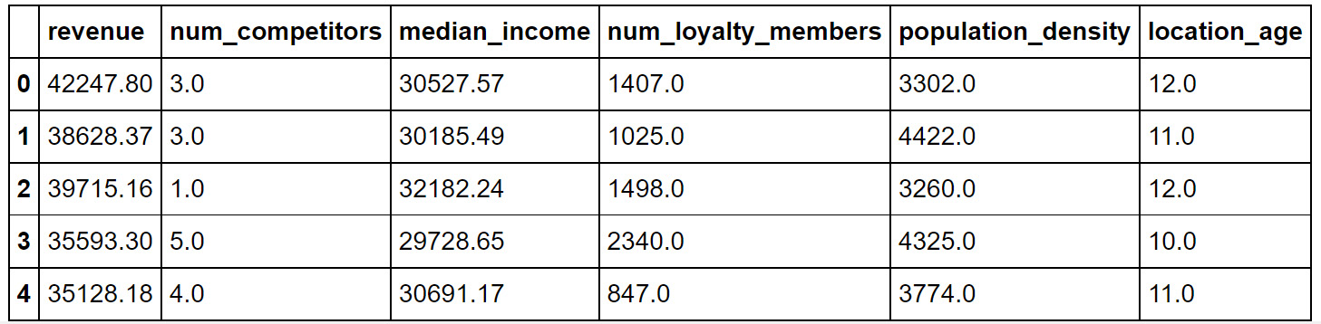
   Figure 6.6: The first five rows of the data in location_rev.csv

2. Import train_test_split from sklearn. Define the y variable as revenue, and X as num_competitors, median_income, num_loyalty_members, population_density, and location_age:

   from sklearn.model_selection import train_test_split

   X = df[['num_competitors',

           'median_income',

           'num_loyalty_members',

           'population_density',

           'location_age']]

   y = df['revenue']

3. Perform a train-test split on the data, using random_state=15, and save the results in X_train, X_test, y_train, and y_test:

   X_train, X_test, y_train, y_test = train_test_split

                                      (X, y, random_state = 15)

4. Import LinearRegression from sklearn, and use it to fit a linear regression model to the training data:

   from sklearn.linear_model import LinearRegression

   model = LinearRegression()

   model.fit(X_train,y_train)

5. Get the model's predictions for the X_test data, and store the result in a variable called predictions:

   predictions = model.predict(X_test)

6. Instead of calculating the RMSE and the MAE yourselves, you can import functions from sklearn to do this for you. Note that sklearn only contains a function to calculate the MSE, so we need to take the root of this value to get the RMSE (that's where the 0.5 comes in). Use the following code to calculate the RMSE and MAE:

   from sklearn.metrics import mean_squared_error,

   mean_absolute_error

   print('RMSE: ' +

         str(mean_squared_error(predictions, y_test)**0.5))

   print('MAE: ' +

         str(mean_absolute_error(predictions, y_test)))

   This should result in the following values:

   RMSE: 5133.736391468814

   MAE: 4161.387875602789

7. Now, rebuild the model after dropping num_competitors from the predictors and evaluate the new model. Create X_train2 and X_test2 variables by dropping num_competitors from X_train and X_test. Train a model using X_train2 and generate new predictions from this model using X_test2:

   X_train2 = X_train.drop('num_competitors', axis=1)

   X_test2 = X_test.drop('num_competitors', axis=1)

   model.fit(X_train2, y_train)

   predictions2 = model.predict(X_test2)

8. Calculate the RMSE and MAE for the new model's predictions and print them out, as follows:

   print('RMSE: ' +

         str(mean_squared_error(predictions2, y_test)**0.5))

   print('MAE: ' +

         str(mean_absolute_error(predictions2, y_test)))

   This should result in the following output:

   RMSE: 5702.030002037039

   MAE: 4544.416946418695

   Note that both values are higher than the values we calculated for the previous model. This means that dropping num_competitors from our model increased the error in our model on the test set. In other words, our model was more accurate when it contained num_competitors. Thus, the intuition by the marketing team was not correct.

Thus, we can see how the MAE and the RMSE can be used to determine the features that are important to have in a model and those that have little impact on performance and can therefore be left out.

In the next activity, you will use the same concept on a marketing dataset to find out the most important variables. Recall that finding the important variables means that less important variables can be dropped, which will add up to the robustness of the model and also reduce the computation time.

Activity 6.01: Finding Important Variables for Predicting Responses to a Marketing Offer

You have been given some data regarding a company's marketing campaign, wherein discounts were offered for various products. You are interested in building a model that predicts the number of responses to an offer. It should also provide information about how much of a discount the offer included (offer_discount), how many customers the offer reached (offer_reach), and a value representing the offer quality that the marketing team assigned to that offer (offer_quality). You want to build a model that is accurate but does not contain unnecessary variables. Use the RMSE to evaluate how the model performs when all variables are included and compare this to what happens when each variable is dropped from the model. This will then help in finding the most important variables for predicting the number of responses to a marketing offer. Follow the steps given here:

1. Import pandas, read in the data from offer_responses.csv, and use the head function to view the first five rows of the data. Your output should appear as follows:

   Figure 6.7: The first five rows of the offer_responses data

   Note

   You can download offer_responses.csv by clicking the following link: https://packt.link/M0wuH.

2. Import train_test_split from sklearn and use it to split the data into training and test sets, using responses as the y variable and all others as the predictor (X) variables. Use random_state=10 for the train-test split.
3. Import LinearRegression and mean_squared_error from sklearn. Fit the model to the training data (using all the predictors), get predictions from the model on the test data, and print out the calculated RMSE on the test data. The RMSE with all variables should be approximately 966.2461828577945.
4. Create X_train2 and X_test2 by dropping offer_quality from X_train and X_test. Train and evaluate the RMSE of the model using X_train2 and X_test2. The RMSE without offer_quality should be approximately 965.5346123758474.
5. Perform the same sequence of steps from step 4, but this time dropping offer_discount instead of offer_quality. The RMSE without offer_discount should be approximately 1231.6766556327284.
6. Perform the same sequence of steps, but this time dropping offer_reach. The RMSE without offer_reach should be approximately 1185.8456831644114.

   Note

   The solution to this activity can be found via this link.

Using Recursive Feature Selection for Feature Elimination

So far, we have discussed two important evaluation metrics – the MAE and RMSE. We also saw how these metrics can be used with the help of the scikit-learn library and how a change in the values of these metrics can be used as an indicator of a feature's importance. However, if you have a large number of features, removing one feature at a time would become a very tedious job, and this is where RFE comes into the picture. When a dataset contains features (all columns, except the column that we want to predict) that either are not related to the target column or are related to other columns, the performance of the model can be adversely affected if all the features are used for model training. Let's understand the basic reasoning behind this.

For example, consider that you want to predict the number of sales of a product given the cost price of the product, the discount available, the selling price of the product, and the date when the product was first launched on the market. As you can expect, the launch date of the original product will not affect the current sales of the product. It means that the feature (launch date of the original product) is not related to the target column (sales of the product). Similarly, the cost price of the product becomes a piece of redundant information if the selling price and discount are already available, which is an example of the second case, in which one column is related to other columns.

When one or more features have a low correlation (dependency between two columns) with the target column, this means that these columns are not going to provide any useful information to the model. However, if we still include them while training the model, the model will be forced to (incorrectly) learn that these columns have some effect on the target column. This can result in overfitting, in which the model will work very well for the training dataset; however, it will show poor performance on the test dataset.

A similar scenario can occur when features have a high correlation. In such a case, the model will overfit the redundant information provided by correlated columns. To avoid such situations, it is recommended to remove extraneous columns (variables that are not related to the outcome of interest) from the dataset before training the model.

In this chapter, we will discuss a powerful technique of feature elimination referred to as RFE. As the name suggests, RFE is a recursive technique that works by removing one feature at a time and compares the effect of removing a feature on the performance of the model. Based on this comparison, the feature that has a minimum adverse effect (or a maximum positive effect) on the model performance is removed, and the process goes on. As you may have understood, this is very similar to the process we followed in the previous activity. In terms of implementation, RFE is part of the scikit-learn package and can be used as follows:

1. First, import RFE from the scikit-learn package:

   from sklearn.feature_selection import RFE

2. Next, create an RFE instance while specifying how many features you want to select. For example, if you want to select 5 features, you will use the following code:

   rfe = RFE(estimator=LinearRegression(), n_features_to_select=5)

3. Fit the RFE model on the training dataset:

   rfe.fit(X_train,y_train)

4. You can then find out which columns were selected by RFE, and which were not, using the following code:

   for featureNum in range(X_train.shape[1]):

     # If feature was selected

     if rfe.support_[featureNum] == True:

       # Print feature name and rank

       print("Feature: {}, Rank:{}"

             .format(X_train.columns[featureNum],

                     rfe.ranking_[featureNum]))

   You will get the following output:

   Feature: offer_quality, Rank:1 Feature: offer_discount, Rank:1 Feature: offer_reach, Rank:1

Now, let's get some hands-on experience of using RFE in the next exercise. We will reuse the code we studied here for RFE in this next exercise.

Exercise 6.02: Using RFE for Feature Selection

For this exercise, you've been given data of the revenue of stores at different locations, and a series of 20 scores based on internal metrics in the 20scores.csv file. You aren't told what the scores mean, but are asked to build a predictive model that uses as few of these scores as possible without sacrificing the ability to predict the location revenue.

Note

You can get the 20scores.csv file at the following link: https://packt.link/KfBrK.

1. Import pandas, read the data from 20scores.csv into a DataFrame called df, and display the first five rows of data using the head function:

   import pandas as pd

   df = pd.read_csv('20scores.csv')

   df.head()

   Note

   Make sure you change the path (emboldened) to the CSV file based on its location on your system. If you're running the Jupyter notebook from the same directory where the CSV file is stored, you can run the preceding code without any modifications.

   You should see the following output:

   

   Figure 6.8: The first five rows of the 20scores.csv data

   Note

   The preceding image does not contain all the columns of the DataFrame. The image is for demonstration purposes only.

2. Extract the target variable (y) and the predictor variable (X) from the data:

   x_cols = df.columns[1:]

   X = df[x_cols]

   y = df['revenue']

3. Import train_test_split and perform a train-test split on the data with random_state=10, storing revenue in the y variable and all other features in the X variable:

   from sklearn.model_selection import train_test_split

   X_train, X_test, y_train, y_test = train_test_split

                                      (X, y, random_state = 10)

4. Import LinearRegression from sklearn and fit a linear regression model on the training data:

   from sklearn.linear_model import LinearRegression

   model = LinearRegression()

   model.fit(X_train,y_train)

5. Look at the model's coefficients using the following code:

   model.coef_

   You should get the following result:

   

   Figure 6.9: Model's coefficients

   Note that all of these values are non-zero. Therefore, the model is using all variables.

6. Now import RFE from sklearn. Use a LinearRegression model as the estimator, which RFE will use in every iteration. Moreover, you will need to specify the number of features you want to select. For now, keep only five features:

   from sklearn.feature_selection import RFE

   rfe = RFE(estimator=LinearRegression(), n_features_to_select=5)

7. Train the RFE model you just created in the previous step on the training data using the following command:

   rfe.fit(X_train,y_train)

   This will provide the following output:

   RFE(estimator=LinearRegression(copy_X=True, fit_intercept=True, n_jobs=None, normalize=False), n_features_to_select=5, step=1, verbose=0)

   Note

   The output may vary from system to system.

8. Print the columns that were selected by RFE along with their ranks:

   for featureNum in range(X_train.shape[1]):

     # If feature was selected

     if rfe.support_[featureNum] == True:

       # Print feature name and rank

       print("Feature: {}, Rank: {}"

             .format(X_train.columns[featureNum],

                     rfe.ranking_[featureNum]))

   The output obtained for this code is given here:

   Feature: score0, Rank: 1

   Feature: score9, Rank: 1

   Feature: score12, Rank: 1

   Feature: score17, Rank: 1

   Feature: score19, Rank: 1

   Notice that only five features were selected by RFE and that all of those features were given a rank 1, meaning that RFE considered all five features to be equally important.

9. Using the preceding information, now create a reduced dataset having only the columns selected by RFE:

   X_train_reduced = X_train[X_train.columns[rfe.support_]]

   X_test_reduced = X_test[X_train.columns[rfe.support_]]

10. Next, use the reduced training dataset to fit a new linear regression model:

    rfe_model = LinearRegression()

    rfe_model.fit(X_train_reduced,y_train)

11. Import mean_squared_error from sklearn and use it to calculate the RMSE of the linear regression model on the test data:

    from sklearn.metrics import mean_squared_error

    predictions = model.predict(X_test)

    print(mean_squared_error(predictions, y_test)**0.5)

    The output should be similar to 491.78833768572633.

12. Similarly, calculate the RMSE of the model generated in step 9 on the test data:

    rfe_predictions = rfe_model.predict(X_test_reduced)

    print(mean_squared_error(rfe_predictions, y_test)**0.5)

    The output should be similar to 487.6184171986599.

You can observe that, although the reduced dataset obtained using RFE only has five features, its RMSE is lower than the linear model that uses all of them. This shows that it has not lost any predictive power, even though it has greatly simplified the model by removing variables.

In the next activity, we will use RFE to find out the top three features for predicting customer spend. This will give you an insight into how RFE can be used in marketing problems where a larger number of columns are commonly present.

Activity 6.02: Using RFE to Choose Features for Predicting Customer Spend

You've been given the following information (features) regarding various customers:

prev_year_spend: How much they spent in the previous year

days_since_last_purchase: The number of days since their last purchase

days_since_first_purchase: The number of days since their first purchase

total_transactions: The total number of transactions

age: The customer's age

income: The customer's income

engagement_score: A customer engagement score, which is a score created based on customers' engagement with previous marketing offers.

You are asked to investigate which of these is related to the customer spend in the current year (cur_year_spend). You'll also need to create a simple linear model to describe these relationships.

Follow the steps given here:

1. Import pandas, use it to read in the data in customer_spend.csv, and use the head function to view the first five rows of data. The output should appear as follows:

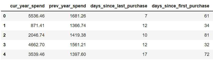
   Figure 6.10: The first five rows of customer_spend.csv

   Note

   You can download the customer_spend.csv file by clicking the following link: https://packt.link/tKJn8.

2. Use train_test_split from sklearn to split the data into training and test sets, with random_state=100 and cur_year_spend as the y variable:
3. Use RFE to obtain the three most important features and obtain the reduced versions of the training and test datasets by using only the selected columns.
4. Train a linear regression model on the reduced training dataset and calculate the RMSE value on the test dataset.

   The RMSE value should be approximately 1075.9083016269915.

   Note

   The solution to this activity can be found via this link.

Tree-Based Regression Models

In the preceding activity, you were able to identify the three most important features that could be used to predict customer spend. Now, imagine doing the same by removing each feature one at a time and finding out the RMSE. RFE aims to remove the redundant task of going over each feature by doing it internally, without forcing the user to put in the effort to do it manually.

So far, we have covered linear regression models. Now it's time to take it up a notch by discussing some tree-based regression models.

Linear models are not the only type of regression models. Another powerful technique is the use of regression trees. Regression trees are based on the idea of a decision tree. A decision tree is a bit like a flowchart, where, at each step, you ask whether a variable is greater than or less than some value. After flowing through several of these steps, you reach the end of the tree and receive an answer for what value the prediction should be. The following figure illustrates the working of regression trees. For example, if you want to predict the age of a person with a height of 1.7 m and a weight of 80 kg, then using the regression tree (left), since the height is less than 1.85m, you will follow the left branch. Similarly, since the weight is less than 90 kg, you will follow the left branch and end at 18. This means that the age of the person is 18 years:

Figure 6.11: A regression tree (left) and how it parses the feature space into predictions

Decision trees are interesting because they can pick up on trends in data that linear regression might miss or capture poorly. Whereas linear models assume a simple linear relationship between predictors and an outcome, regression trees result in more complex functions, which can fit certain kinds of relationships more accurately.

The implementation stays the same as the linear regression model in scikit-learn, the only difference being that this time, instead of importing LinearRegression, you will need to import DecisionTreeRegressor, as shown here:

from sklearn.tree import DecisionTreeRegressor

You can then create an instance of the decision tree regressor. In the following code, you can change the maximum depth of the tree as per requirements:

tree_model = DecisionTreeRegressor(max_depth=2)

One important parameter for regression trees is the maximum depth of the tree. The more depth that a tree is allowed, the more complex a relationship it can model. While this may sound like a good thing, choosing too high a maximum depth can lead to a model that is highly overfitted to the data. In fact, the tendency to overfit is one of the biggest drawbacks of regression trees. That's where random forests come in handy.

Random Forests

To overcome the issue of overfitting, instead of training a single tree to find patterns in data, many trees are trained over random subsets of the data. The predictions of these trees are then averaged to produce a prediction. Combining trees together in this way is called a random forest. This technique has been found to overcome many of the weaknesses associated with regression trees. The following figure illustrates an ensemble of tree models, each of whose predictions are averaged to produce the ensemble's predictions. We see that n number of trees are trained over random subsets of data. Then, the mean of the predictions from those trees is the desired prediction:

Figure 6.12: An ensemble of tree models

Random forests are based on the idea of creating an ensemble, which is where multiple models are combined to produce a single prediction. This is a powerful technique that can often lead to very good outcomes. In the case of random forests, creating an ensemble of regression trees together in this way has been shown to not only decrease overfitting but also to produce very good predictions in a wide variety of scenarios.

Similar to the regression trees discussed in the previous section, random forests can be created using the following steps with the help of the scikit-learn library.

First, import RandomForestRegressor from the scikit-learn module:

from sklearn.module import RandomForestRegressor

You can then create an instance of the random forest regressor. In the following code, you can change the maximum depth of the trees present in the random forest as per your requirements:

forest_model = RandomForestRegressor(max_depth=2)

Because tree-based methods and linear regression are so drastically different in the way they fit to data, they often work well in different circumstances. When the relationships in data are linear (or close to it), linear models will tend to produce more accurate predictions, with the bonus of being easy to interpret. When relationships are more complex, tree-based methods may perform better. For example, the profit made by a firm and the profit made by each advertisement run by them is a linear relationship. If the profit made by each ad doubles, the overall profit of the firm will also double. However, the number of ads doesn't necessarily have to follow a linear relationship with the profit, as you can have 100 ads performing poorly, versus only one ad performing really well. This is a complex, or non-linear, relationship. Testing each and choosing the best model for the job requires evaluating the models based on their predictive accuracy with a metric such as the RMSE. The choice is ultimately dependent on the data you are working on.

For example, if you realize during the initial stages of data analysis (let's say you notice that the data points are approximately following a linear curve) that a linear model will fit the data accurately, it's better to go for a linear regression model rather than the more complex tree-based regression models. In the worst-case scenario, you can try out both approaches and choose the most accurate one.

Now it is time to put the skills we learned to use by using tree-based regression models to predict the customers' spend given their ages.

Exercise 6.03: Using Tree-Based Regression Models to Capture Non-Linear Trends

In this exercise, you'll look at a very simple dataset where you have data on customers' spend and their ages. You want to figure out how spending habits change with age in your customers, and how well different models can capture this relationship. Having a model like this can help in building age-specific website patterns for your customers since you will be able to recommend products that suit the customers' spend levels.

Perform the following steps to achieve the aim of this exercise:

1. Import pandas and use it to read in the data in age_spend.csv. Use the head function to view the first five rows of the data:

   import pandas as pd

   df = pd.read_csv('age_spend.csv')

   df.head()

   Note

   Make sure you change the path (emboldened) to the CSV file based on its location on your system. If you're running the Jupyter notebook from the same directory where the CSV file is stored, you can run the preceding code without any modifications.

   Your output will appear as follows:

   

   Figure 6.13: The first five rows of the age_spend data

   Note

   You can download the age_spend.csv file from the following link: https://packt.link/NxEiK.

2. Extract the target variable (y) and the predictor variable (X) from the data:

   X = df[['age']]

   y = df['spend']

3. Import train_test_split from sklearn and use it to perform a train-test split of the data, with random_state=10 and y being the spend and X being the age:

   from sklearn.model_selection import train_test_split

   X_train, X_test, y_train, y_test = train_test_split

                                      (X, y, random_state = 10)

4. Import DecisionTreeRegressor from sklearn and fit two decision trees to the training data, one with max_depth=2 and one with max_depth=5:

   from sklearn.tree import DecisionTreeRegressor

   max2_tree_model = DecisionTreeRegressor(max_depth=2)

   max2_tree_model.fit(X_train,y_train)

   max5_tree_model = DecisionTreeRegressor(max_depth=5)

   max5_tree_model.fit(X_train,y_train)

5. Import LinearRegression from sklearn and fit a linear regression model to the training data, as shown:

   from sklearn.linear_model import LinearRegression

   model = LinearRegression()

   model.fit(X_train,y_train)

   You will get the following output:

   LinearRegression(copy_X=True, fit_intercept=True, n_jobs=None, normalize=False)

   Note

   The output may vary from system to system.

6. Import mean_squared_error from sklearn. For the linear model and the two regression tree models, get predictions from the model for the test set and use these to calculate the RMSE. Use the following code:

   from sklearn.metrics import mean_squared_error

   linear_predictions = model.predict(X_test)

   print('Linear model RMSE: ' +

         str(mean_squared_error(linear_predictions, y_test)**0.5))

   max2_tree_predictions = max2_tree_model.predict(X_test)

   print('Tree with max depth of 2 RMSE: ' +

         str(mean_squared_error(max2_tree_predictions, y_test)**0.5))

   max5_tree_predictions = max5_tree_model.predict(X_test)

   print('tree with max depth of 5 RMSE: ' +

         str(mean_squared_error(max5_tree_predictions, y_test)**0.5))

   You should get the following RMSE values for the linear and decision tree models with maximum depths of 2 and 5, respectively: 159.07639273785358, 125.1920405443602, and 109.73376798374653.

   Notice that the linear model has the largest error, the decision tree with a maximum depth of 2 does better, and the decision tree with a maximum depth of 5 has the lowest error of the three.

7. Import matplotlib. Create a variable called ages to store a DataFrame with a single column containing ages from 18 to 70, so that we can have our models give us their predictions for all these ages:

   import matplotlib.pyplot as plt

   %matplotlib inline

   ages = pd.DataFrame({'age':range(18,70)})

8. Create a scatter plot with the test data and, on top of it, plot the predictions from the linear regression model for the range of ages. Plot with color='k' and linewidth=5 to make it easier to see:

   plt.scatter(X_test.age.tolist(), y_test.tolist(), color='gray')

   plt.plot(ages,model.predict(ages), color='k', linewidth=5,

            label="Linear Regression")

   plt.xlabel("age")

   plt.ylabel("spend")

   plt.show()

   Note

   In Steps 8, 9, 10, 13, and 14, the values gray and k for the attribute color (emboldened) is used to generate graphs in grayscale. You can also refer to the following document to get the code for the colored plot and the colored output: http://packt.link/NOjgT.

   The following plot shows the predictions of the linear regression model across the age range plotted on top of the actual data points:

   

   Figure 6.14: The predictions of the linear regression model

   You can see that the linear regression model just shows a flat line across the ages; it is unable to capture the fact that people aged around 40 spend more, while people younger and older than 40 spend less.

9. Create another scatter plot with the test data, this time plotting the predictions of the max2_tree model on top with color='k' and linewidth=5:

   plt.scatter(X_test.age.tolist(), y_test.tolist(), color='gray')

   plt.plot(ages,max2_tree_model.predict(ages),

            color='k',linewidth=5,label="Tree with max depth 2")

   plt.xlabel("age")

   plt.ylabel("spend")

   plt.show()

   The following plot shows the predictions of the regression tree model with max_depth of 2 across the age range plotted on top of the actual data points:

   

   Figure 6.15: The predictions of the regression tree model with max_depth of 2

   This model does a better job of capturing the relationship, though it does not capture the sharp decline in the oldest or youngest populations.

10. Create one more scatter plot with the test data, this time plotting the predictions of the max5_tree model on top with color='k' and linewidth=5:

    plt.scatter(X_test.age.tolist(), y_test.tolist(), color='gray')

    plt.plot(ages,max5_tree_model.predict(ages), color='k',

             linewidth=5, label="Tree with max depth 5")

    plt.xlabel("age")

    plt.ylabel("spend")

    plt.show()

    The following plot shows the predictions of the regression tree model with max_depth of 5 across the age range plotted on top of the actual data points:

    

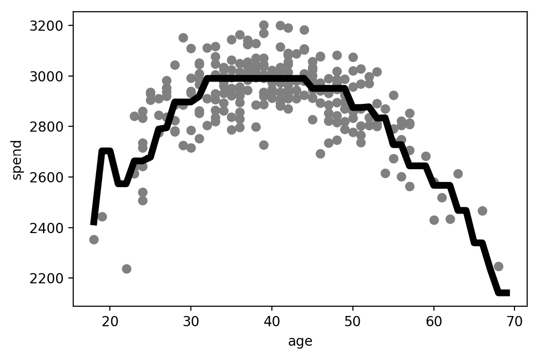
    Figure 6.16: The predictions of the regression tree model with max_depth of 5

    This model does an even better job of capturing the relationship, properly capturing a sharp decline in the oldest or the youngest population.

11. Let's now perform random forest regression on the same data. Import RandomForestRegressor from sklearn. Fit two random forest models with random_state=10, one with max_depth=2 and the other with max_depth=5, and save these as max2_forest_model and max5_forest_model, respectively:

    from sklearn.ensemble import RandomForestRegressor

    max2_forest_model = RandomForestRegressor

                        (max_depth=2, random_state=10)

    max2_forest_model.fit(X_train,y_train)

    max5_forest_model = RandomForestRegressor

                        (max_depth=5, random_state=10)

    max5_forest_model.fit(X_train,y_train)

    You will get the following output:

    RandomForestRegressor(max_depth=5, random_state=10)

12. Calculate and print the RMSE for the two random forest models using the following code:

    max2_forest_predictions = max2_forest_model.predict(X_test)

    print('Max depth of 2 RMSE: ' +

          str(mean_squared_error(max2_forest_predictions,

                                 y_test)**0.5))

    max5_forest_predictions = max5_forest_model.predict(X_test)

    print('Max depth of 5 RMSE: ' +

          str(mean_squared_error(max5_forest_predictions,

                                 y_test)**0.5))

    The following RMSE values should be obtained for the random forest models with maximum depths of 2 and 5, respectively: 115.51279667457273 and 109.61188562057568. Please note that there might be some minute differences in these values.

    Based on the RMSE values obtained, we can see that the random forest models performed better than regression tree models of the same depth. Moreover, all tree-based regression models outperformed the linear regression model.

13. Create another scatter plot with the test data, this time plotting the predictions of the max2_forest_model model on top with color='k' and linewidth=5:

    plt.scatter(X_test.age.tolist(), y_test.tolist(),color='gray')

    plt.plot(ages,max2_forest_model.predict(ages), color='k',

             linewidth=5, label="Forest with max depth 2")

    plt.xlabel("age")

    plt.ylabel("spend")

    plt.show()

    The following plot shows the predictions of the random forest model with max_depth of 2 across the age range plotted on top of the actual data points:

    

    Figure 6.17: The predictions of the random forest model with max_depth of 2

    We can see that this model captures the data trend better than the decision tree, but still doesn't quite capture the trend at the very high or low ends of our range.

14. Create another scatter plot with the test data, this time plotting the predictions of the max2_forest_model model on top with color='k' and linewidth=5:

    plt.scatter(X_test.age.tolist(), y_test.tolist(), color='gray')

    plt.plot(ages,max5_forest_model.predict(ages), color='k',

             linewidth=5, label="Forest with max depth 5")

    plt.xlabel("age")

    plt.ylabel("spend")

    plt.show()

    The following plot shows the predictions of the random forest model with max_depth of 5 across the age range plotted on top of the actual data points:

    

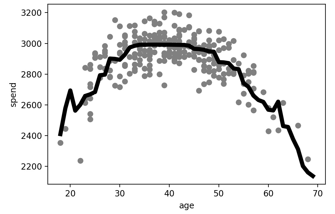
Figure 6.18: The predictions of the random forest model with max_depth of 5

Again, in the model, the greater maximum depth does an even better job of capturing the relationship, properly capturing the sharp decline in the oldest and youngest population groups.

The preceding results can easily be clubbed together to create the plot shown here, which presents a nice comparison of using different max_depth attributes while training the random forest model.

The code used to generate the plot is given here:

plt.figure(figsize=(12,8))

plt.scatter(X_test.age.tolist(), y_test.tolist())

plt.plot(ages,model.predict(ages), color='r', linewidth=5,

         label="Linear Regression")

plt.plot(ages,max2_tree_model.predict(ages), color='g',

         linewidth=5,label="Tree with max depth 2")

plt.plot(ages,max5_tree_model.predict(ages), color='k',

         linewidth=5, label="Tree with max depth 5")

plt.plot(ages,max2_forest_model.predict(ages), color='c',

         linewidth=5, label="Forest with max depth 2")

plt.plot(ages,max5_forest_model.predict(ages), color='m',

         linewidth=5, label="Forest with max depth 5")

plt.legend()

plt.xlabel("age")

plt.ylabel("spend")

plt.show()

You should get the following output:

Figure 6.19: Comparison of using different max_depth values while training the random forest model

In this exercise, you saw that the tree-based models outperformed the linear regression model since the data was non-linear. Among the tree-based models, the random forest model had the lowest RMSE value. You also saw that by increasing the maximum depth from 2 to 5, the curve started fitting the training dataset more tightly. You will explore this part in detail in later chapters. You also saw that for people aged between 20 and 40, the total expenditure increased with age; however, for people aged over 50, the trend was completely the opposite.

Now, let's use the knowledge gained so far to build a regression model to predict the customer spend based on the user data given. You will again have to fit different kinds of regression models and choose the best among those.

Activity 6.03: Building the Best Regression Model for Customer Spend Based on Demographic Data

You are given data of customers' spend at your business and some basic demographic data regarding each customer (age, income, and years of education). You are asked to build the best predictive model possible that can predict, based on these demographic factors, how much a given customer will spend at your business. The following are these high-level steps to solve this activity:

1. Import pandas, read the data in spend_age_income_ed.csv into a DataFrame, and use the head function to view the first five rows of the data. The output should be as follows:

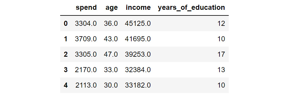
   Figure 6.20: The first five rows of the spend_age_income_ed data

   Note

   You can get the spend_age_income_ed.csv file at the following link: https://packt.link/LGGyB.

2. Perform a train-test split with random_state=10.
3. Fit a linear regression model to the training data.
4. Fit two regression tree models to the data, one with max_depth=2 and one with max_depth=5.
5. Fit two random forest models to the data, one with max_depth=2, one with max_depth=5, and random_state=10 for both.
6. Calculate and print out the RMSE on the test data for all five models.

   The following table summarizes the expected output for all the models. The values you get may not be an exact match with these expected values. You may get a deviation of within 5% of these values.

   

Figure 6.21: Expected outputs for all five models

Note

The solution to this activity can be found via this link.

Summary

In this chapter, we learned how to evaluate regression models. We used residuals to calculate the MAE and RMSE, and then used those metrics to compare models. We also learned about RFE and how it can be used for feature selection. We were able to see the effect of feature elimination on the MAE and RMSE metrics and relate it to the robustness of the model. We used these concepts to verify that the intuitions about the importance of the "number of competitors" feature were wrong in our case study. Finally, we learned about tree-based regression models and looked at how they can fit some of the non-linear relationships that linear regression is unable to handle. We saw how random forest models were able to perform better than regression tree models and the effect of increasing the maximum tree depth on model performance. We used these concepts to model the spending behavior of people with respect to their age.

In the next chapter, we will learn about classification models, the other primary type of supervised learning models.