8. Fine-Tuning Classification Algorithms

Overview

This chapter will help you optimize predictive analytics using classification algorithms such as support vector machines, decision trees, and random forests, which are some of the most common classification algorithms from the scikit-learn machine learning library. Moreover, you will learn how to implement tree-based classification models, which you have used previously for regression. Next, you will learn how to choose appropriate performance metrics for evaluating the performance of a classification model. Finally, you will put all these skills to use in solving a customer churn prediction problem where you will optimize and evaluate the best classification algorithm for predicting whether a given customer will churn or not.

Introduction

Consider a scenario where you are the machine learning lead in a marketing analytics firm. Your firm has taken over a project from Amazon to predict whether or not a user will buy a product during festive season sale campaigns. You have been provided with anonymized data about customer activity on the Amazon website – the number of products purchased, their prices, categories of the products, and more. In such scenarios, where the target variable is a discrete value – for example, the customer will either buy the product or not – the problems are referred to as classification problems. There are a large number of classification algorithms available now to solve such problems and choosing the right one is a crucial task. So, you will first start exploring the dataset to come up with some observations about it. Next, you will try out different classification algorithms and evaluate the performance metrics for each classification model to understand whether the model is good enough to be used by the company. Finally, you will end up with the best classification algorithm out of the entire pool of models you trained, and this model will then be used to predict whether a user will buy a product during the sale.

In this chapter, you'll be working on problems like these to understand how to choose the right classification algorithm by evaluating its performance using various metrics. Picking the right performance metrics and optimizing, fine-tuning, and evaluating the model is an important part of building any supervised machine learning model. Moreover, choosing an appropriate machine learning model is an art that requires experience, and each algorithm has its advantages and disadvantages.

In the previous chapter, you learned about the most common data science pipeline: OSEMN. You also learned how to preprocess, explore, model, and finally, interpret data. This chapter builds upon the skills you learned therein. You will start by using the most common Python machine learning API, scikit-learn, to build a logistic regression model, then you will learn different classification algorithms and the intuition behind them, and finally, you will learn how to optimize, evaluate, and choose the best model.

Support Vector Machines

When dealing with data that is linearly separable, the goal of the Support Vector Machine (SVM) learning algorithm is to find the boundary between classes so that there are fewer misclassification errors. However, the problem is that there could be several decision boundaries (B1, B2), as you can see in the following figure:

Figure 8.1: Multiple decision boundary

As a result, the question arises as to which of the boundaries is better, and how to define better. The solution is to use a margin as the optimization objective. A margin can be described as the distance between the boundary and two points (from different classes) lying closest to the boundary. Figure 8.2 gives a nice visual definition of the margin.

The objective of the SVM algorithm is to maximize the margin. You will go over the intuition behind maximizing the margin in the next section. For now, you need to understand that the objective of an SVM linear classifier is to increase the width of the boundary before hitting a data point. The algorithm first finds out the width of the hyperplane and then maximizes the margin. It chooses the decision boundary that has the maximum margin.

While it might seem too daunting in the beginning, you don't need to worry about this since the algorithm will internally carry out all these tasks and will be able to give you the target class for a given data point. For instance, in the preceding figure, it chooses B1 because it had a larger margin compared to B2. You can refer to the margins for the decision boundaries of B1 and B2 in Figure 8.2:

Note

In geometry, a hyperplane is a subspace whose dimension is one less than that of its ambient space. For example, in the case of a 2D space (for example, Figure 8.1), the hyperplane would be a line.

Figure 8.2: Decision boundary with a different width/margin

The following are the advantages and disadvantages of the SVM algorithm:

Advantages

• SVMs are effective when dealing with high-dimensional data, where the number of dimensions is more than the number of training samples.
• SVMs are known for their use of the kernel function, making it a very versatile algorithm.

  Note

  Kernel methods are mathematical functions used to convert data from lower-dimensional space to higher-dimensional space, or vice versa. The idea behind kernel functions is that data that is not linearly separated in one-dimensional space might be linearly separated in a higher-dimensional space.

Disadvantages

• SVMs do not calculate probability directly, and instead use five-fold cross-validation to calculate probability, which can make the algorithm considerably slow.
• With high-dimensional data, it is important to choose the kernel function and regularization term, which can make the process very slow.

Intuition behind Maximum Margin

Figure 8.3: Geometrical interpretation of maximum margin

The logic behind having large margins in the case of an SVM is that they have a lower generalization error compared to small margins, which can result in overfitted data.

Consider Figure 8.3, where you have data points from two classes –squares and circles. The data points that are closest to the boundary are referred to as support vectors as they are used for calculating the margin. The margin on the left side of the boundary is referred to as the negative hyperplane and the margin on the right side of the boundary is referred to as the positive hyperplane.

Let's consider the positive and negative hyperplane as follows:

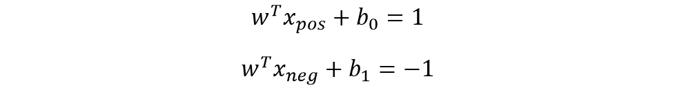
Figure 8.4: Positive and negative hyperplane equation

In the preceding equations:

• w refers to the slope of the hyperplane.
• b0 and b1 refer to the intercepts of the hyperplanes.
• T refers to the transpose.
• xpos and xneg refer to the points through which the positive and negative hyperplanes are passing, respectively.

The preceding equations can also be thought of as an equation of a line: y = mx + c, where m is the slope and c is the intercept. Because of this similarity, SVM is referred to as the SVM linear classifier.

Subtracting the preceding two equations, you get the following:

Figure 8.5: Combined equation of two separate hyperplanes

Normalizing the equation by the vector w, you get the following, where m refers to the data points you have and i refers to the ith data point:

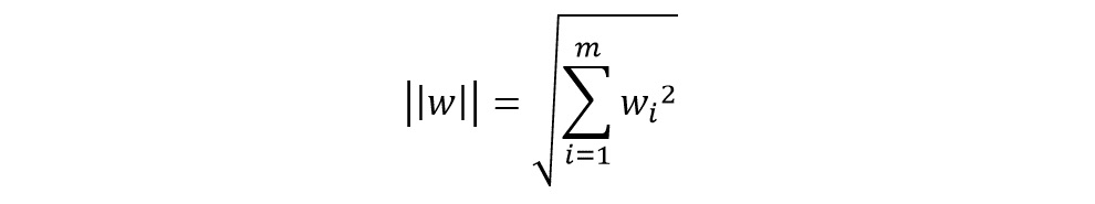
Figure 8.6: Normalized equation

You reduce the preceding equation as follows:

Figure 8.7: Equation for margin m

Now, the objective function is obtained by maximizing the margin within the constraint that the decision boundary should classify all the points correctly.

Now once you have the decision boundary ready, you can use the following equation to classify the points based on which side of the decision boundary they lie on:

Figure 8.8: Equation for separating the data points on a hyperplane

To implement an SVM-based classifier, you can use the scikit-learn module as follows:

1. Import svm from scikit-learn:

   from sklearn import svm

2. Create an instance of the SVM model that will then be used for training on the dataset:

   model = svm.SVC()

   In the preceding function, you can also specify the kernel type (linear, sigmoid, rbf, and so on), the regularization parameter C, the gamma value for the kernel, and so on. You can read the entire list of the parameters available along with their default values here: https://scikit-learn.org/stable/modules/generated/sklearn.svm.SVC.html#sklearn.svm.SVC.

3. Once you have the model instance, you can use model.fit(X_train,y_train) to train the model and model.predict(X) to get the prediction.

So far you have been dealing with the hard margin, which does not leave any space for mistakes. In other words, all instances from one class have to lie on one side of the margin. However, this rigid behavior can affect the generalizability of the model. To resolve this, you can use a soft margin classifier.

Linearly Inseparable Cases

With linearly inseparable cases, such as the one illustrated in the following figure, you cannot use a hard-margin classifier. The solution is to introduce a new kind of classifier, known as a soft-margin classifier, using the slack variable ξ. The slack variable converts the equations discussed in the previous section into inequalities by allowing for some mistakes, as shown in Figure 8.9:

Figure 8.9: Linearly inseparable data points

Note

The hard margin refers to the fitting of a model with zero errors; hence you cannot use a hard-margin classifier for the preceding figure. A soft margin, on the other hand, allows the fitting of a model with some error, as highlighted by the points circled in blue in the preceding figure.

A soft-margin SVM works by doing the following:

1. Introducing the slack variable
2. Relaxing the constraints
3. Penalizing the relaxation

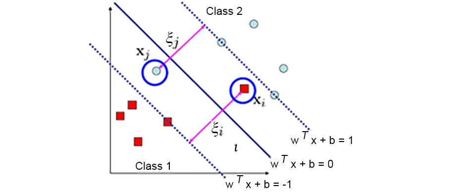
Figure 8.10: Using the slack variable ξ for linearly inseparable data

The linear constraints can be changed by adding the slack variable to the equation in Figure 8.5 as follows:

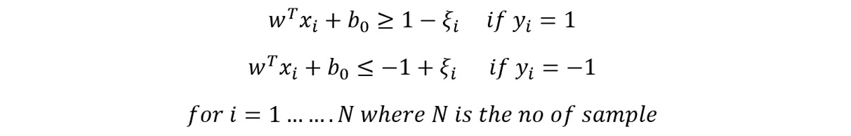
Figure 8.11: Linear constraints for maximizing margin with slack variable ξ

The objective function for linearly inseparable data points is obtained by minimizing the following:

Figure 8.12: Objective function to be minimized

Here, C is the penalty cost parameter (regularization). This parameter C can be specified as a parameter when calling the svm.SVC() function, as discussed in the previous section.

Linearly Inseparable Cases Using the Kernel

In the preceding example, you saw how you can use a soft-margin SVM to classify datasets using the slack variable. However, there can be scenarios where it is quite hard to separate data. For example, in the following figure, it would be impossible to have a decision boundary using the slack variable and a linear hyperplane:

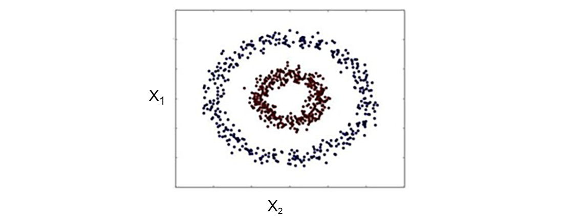
Figure 8.13: Linearly inseparable data points

In this scenario, you can use the concept of a kernel, which creates a nonlinear combination of original features (X1, X2) to project to a higher-dimensional space via a mapping function, φ, to make it linearly separable:

Figure 8.14: Geometric interpretation and equation for projection from a low to a high dimension

The problem with this explicit feature mapping is that the dimensionality of the feature can be very high, which makes it hard to represent it explicitly in memory. This is mitigated using the kernel trick. The kernel trick basically replaces the dot product xiT xj with a kernel φ xiTφ(xj), which can be defined as follows:

Figure 8.15: Kernel function

There are different types of kernel functions, namely:

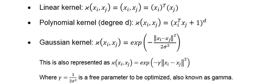
Figure 8.16: Different kernel functions

A kernel can also be interpreted as a similarity function and lies between 0 (an exactly dissimilar sample) and 1 (a sample that is exactly the same).

In scikit-learn, the following kernel functions are available:

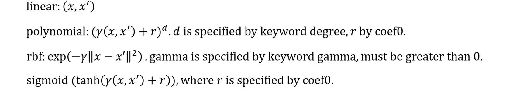
Figure 8.17: Different kernel functions implemented in scikit-learn

So, you can use them as follows:

svm.SVC(kernel='poly', C=1)

Here, you can change the kernel using different kernel functions such as 'linear', 'poly', and so on, which is similar to what we have described in Figure 8.17.

Now that you have gone through the details of the SVM algorithm and how to implement the SVM classifier using the scikit-learn module, it's time to put the skills to use by training an SVM classifier on the Shill Bidding dataset.

Exercise 8.01: Training an SVM Algorithm Over a Dataset

In this exercise, you will work with the Shill Bidding dataset, the file for which is named Shill_Bidding_Dataset.csv. You can download this dataset from the following link: https://packt.link/GRn3G. This is the same dataset you were introduced to in Exercise 7.01, Comparing Predictions by Linear and Logistic Regression on the Shill Bidding Dataset. Your objective is to use this information to predict whether an auction depicts normal behavior or not (0 means normal behavior and 1 means abnormal behavior). You will use the SVM algorithm to build your model:

1. Import pandas, numpy, train_test_split, cross_val_score, and svm from the sklearn library:

   import pandas as pd

   from sklearn.model_selection import train_test_split

   from sklearn import svm

   from sklearn.model_selection import cross_val_score

   import numpy as np

2. Read the dataset into a DataFrame named data using pandas, as shown in the following snippet, and look at the first few rows of the data:

   data=pd.read_csv("Shill_Bidding_Dataset.csv")

   Note

   If the CSV file you downloaded is stored in a different directory from where you're running the Jupyter notebook, you'll need to change the emboldened path in the preceding command.

3. First, remove the columns that are irrelevant to the case study. These are ID columns and thus will be unique to every entry. Because of their uniqueness, they won't add any value to the model and thus can be dropped:

   # Drop irrelevant columns

   data.drop(["Record_ID","Auction_ID","Bidder_ID"],axis=1,

             inplace=True)

   data.head()

   Your output will look as follows:

   

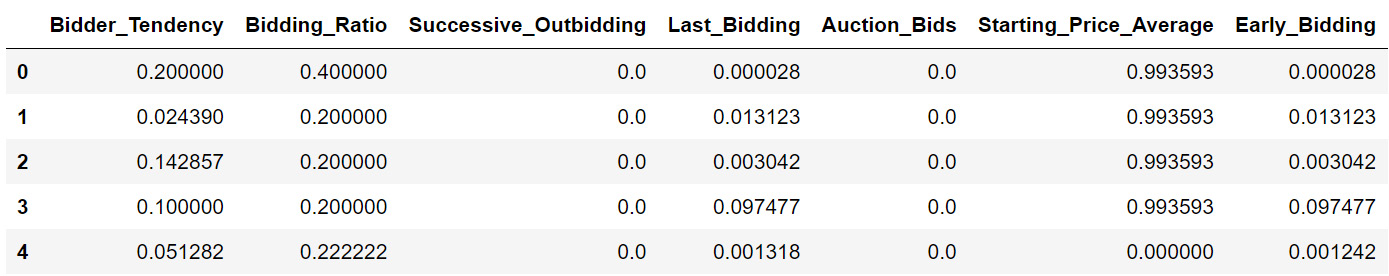
   Figure 8.18: First few rows of auction data

4. Check the data types, as follows:

   data.dtypes

   You'll get the following output. Glancing at it, you can see that all the columns have an appropriate data type so you don't have to do any further preprocessing here:

   

   Figure 8.19: Data type of the auction dataset

5. Look for any missing values using the following code:

   data.isnull().sum() ### Check for missing values

   You should get the following output:

   

   Figure 8.20: Checking for missing values

   Now that there are no missing values, train the SVM algorithm over the dataset.

6. Split the data into train and test sets and save them as X_train, X_test, y_train, and y_test as shown:

   target = 'Class'

   X = data.drop(target,axis=1)

   y = data[target]

   X_train, X_test, y_train, y_test = train_test_split

                                      (X.values,y,test_size=0.50,

                                       random_state=123,

                                       stratify=y)

7. Fit a linear SVM model with C=1:

   Note

   C is the penalty cost parameter for regularization. Please refer to the objective function for linearly inseparable data points in the SVM algorithm mentioned in Figure 8.12.

   clf_svm=svm.SVC(kernel='linear', C=1)

   clf_svm.fit(X_train,y_train)

   You will get the following output:

   SVC(C=1, kernel='linear')

   Note

   The output may vary slightly depending on your system.

8. Calculate the accuracy score using the following code:

   clf_svm.score(X_test, y_test)

   You will get the following output:

   0.9775387535590003

   For the auction dataset, the SVM classifier will score an accuracy of around 97.75%. This implies it can predict 97.75% of the test data accurately.

Decision Trees

Decision trees are mostly used for classification tasks. They are a non-parametric form of supervised learning method, meaning that unlike in SVM where you had to specify the kernel type, C, gamma, and other parameters, there are no such parameters to be specified in the case of decision trees. This also makes them quite easy to work with. Decision trees, as the name suggests, use a tree-based structure for making a decision (finding the target variable). Each "branch" of the decision tree is made by following a rule, for example, "is some feature more than some value? – yes or no." Decision trees can be used both as regressors and classifiers with minimal changes. The following are the advantages and disadvantages of using decision trees for classification:

Advantages

• Decision trees are easy to understand and visualize.
• They can handle both numeric and categorical data.
• The requirement for data cleaning in the case of decision trees is very low since they can handle missing data.
• They are non-parametric machine learning algorithms that make no assumptions regarding space distribution and classifier structures.
• It's a white-box model, rather than a black-box model like neural networks, and can explain the logic of the split using Boolean values.

Disadvantages

• Decision trees tend to overfit data very easily, and pruning is required to prevent overfitting of the model. As a quick recap, overfitting occurs when the model starts to learn even the randomness in the data points, instead of focusing only on the inherent pattern in the data points. This results in the model losing its generalizability.
• They are not suitable for imbalanced data, where you may have a biased decision tree. A decision tree would try to split the node based on the majority class and therefore doesn't generalize very well. The remedy is to balance your data before applying decision trees. Most medical datasets, for example, the dataset on the number of polio patients in India, are imbalanced datasets. This is because the percentage of people who have the illness is extremely small compared to those who don't have the illness.

Similar to SVM classifiers, it is very easy to implement a decision tree classifier using the scikit-learn module:

1. Import the tree sub-module from the scikit-learn module:

   from sklearn import tree

2. Also, import the export_graphviz function that will be used to visualize the created tree:

   from sklearn.tree import export_graphviz

3. To plot the tree in Jupyter Notebooks, import the Image submodule:

   from IPython.display import Image

4. You will also need to import the StringIO module to convert the text into an image:

   from sklearn.externals.six import StringIO

5. Create a decision tree classifier instance:

   clf_tree = tree.DecisionTreeClassifier()

   You can fit the decision tree classifier on the training dataset using clf_tree.fit(X_train,y_train).

6. Similarly, in order to find the prediction using the classifier, use clf_tree.predict(X).
7. Once the decision tree is trained, use the following code to plot it using the export_graphviz function:

   dot_data = StringIO()

   export_graphviz(clf_tree, out_file=dot_data,

                   filled=True, rounded=True,

                   class_names=['Positive','Negative'],

                   max_depth = 3,

                   special_characters=True,

                   feature_names=X.columns.values)

   graph = pydotplus.graph_from_dot_data(dot_data.getvalue())

   Image(graph.create_png())

   Here, class_names is a list that stores the names of the target variable classes. For example, if you want to predict whether a given person has polio or not, the target class names can be Positive or Negative.

Now that we have discussed decision trees and their implementation, let's use them in the next exercise on the same Shill Bidding dataset we used earlier.

Exercise 8.02: Implementing a Decision Tree Algorithm over a Dataset

In this exercise, you will use decision trees to build a model over the same auction dataset that you used in the previous exercise. This practice of training different classifiers on the same dataset is very common whenever you are working on any classification task. Training multiple classifiers of different types makes it easier to pick the right classifier for a task.

Note

Ensure that you use the same Jupyter notebook as the one used for the preceding exercise.

1. Import tree, graphviz, StringIO, Image, export_graphviz, and pydotplus:

   import graphviz

   from sklearn import tree

   from sklearn.externals.six import StringIO

   from IPython.display import Image

   from sklearn.tree import export_graphviz

   import pydotplus

2. Fit the decision tree classifier using the following code:

   clf_tree = tree.DecisionTreeClassifier()

   clf_tree = clf_tree.fit(X_train, y_train)

3. Plot the decision tree using a graph. In this plot, you will be using export_graphviz to visualize the decision tree. You will use the output of your decision tree classifier as your input clf. The target variable will be the class_names, that is, Normal or Abnormal.

   dot_data = StringIO()

   export_graphviz(clf_tree, out_file=dot_data,

                   filled=True, rounded=True,

                   class_names=['Normal','Abnormal'],

                   max_depth = 3,

                   special_characters=True,

                   feature_names=X.columns.values)

   graph = pydotplus.graph_from_dot_data(dot_data.getvalue())

   Image(graph.create_png())

   The output of the preceding snippet will be a graphic visualization of the decision tree to a depth of 3. While it might not seem very intuitive in beginning, it serves an interesting purpose of displaying what rules are being used at each node. For example, in the very beginning, the Successive_Outbidding feature is compared. If the value is less than or equal to 0.25, you follow the left branch, otherwise, you follow the right branch. Please note that the output can vary slightly since decision trees use randomness to fit the model.

   

   Figure 8.21: Graphic visualization of the decision tree

4. Calculate the accuracy score using the following code:

   clf_tree.score(X_test, y_test)

   You should get an output close to 0.9981, which means that our decision tree classifier scores an accuracy of around 99.81%. Hence our classifier can predict 99.81% of the test data correctly.

While we have discussed the basics of decision trees and their implementation, we are yet to go into the theoretical details of the algorithm. In the following sections, we will first cover the terminology related to decision trees and how the decision tree algorithm works.

Important Terminology for Decision Trees

Decision trees get their name from the inverted tree-like structure they follow. Now, in a normal tree, the bottom part is the root, and the topmost part is the leaf of the tree. Since a decision tree follows the reverse structure, the topmost node is referred to as the root node. A node, in simple terms, is the smallest block in the decision tree. Every node has a certain rule that decides where to go next (which branch to follow). The last nodes or the terminal nodes of the decision tree are called leaves. This is where the target variable prediction happens. When a new input is provided for prediction, it first goes to the root node and then moves down to the leaf node for prediction.

As you can understand here, there is a large number of decision trees that can be created out of the features available in a dataset. In the next section, you will see how a specific feature is selected at a node, which then helps in selecting one decision tree out of the large sample space.

Decision Tree Algorithm Formulation

Decision trees use multiple algorithms to split at the root node or sub-node. A decision tree goes through all of the features and picks the feature on which it can get the most homogeneous sub-nodes. For classification tasks, it decides the most homogeneous sub-nodes based on the information gained. Let's discuss information gain first. In short, each of the nodes in a decision tree represents a feature, each of the branches represents a decision rule, and each of the leaves represents an outcome. It is a flow-like structure.

Information gain

This gives details on how much "information" a feature will hold about the class. Features that are perfectly separable or partitioned will give us maximum information, while features that are not perfectly separable or partitioned will give us less information:

Figure 8.22: Information gain formula

Here, IG = information gain, I = impurity, f = feature, Dp = parent dataset, Dleft = left child dataset, Dright = right child dataset, Np = total number of samples in the parent dataset, Nleft = number of samples in the left child dataset, and Nright = number of samples in the right child dataset.

The impurity can be calculated using any of the following three criteria:

• Gini impurity
• Entropy
• Misclassification rate

Let's look into each criterion one by one.

Gini impurity

The Gini index can be defined as the criterion that would minimize the probability of misclassification:

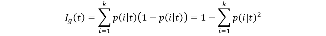
Figure 8.23: Gini impurity

Here, k = number of classes and p(i│t) = proportion of samples that belong to class k for a particular node t.

For a two-class problem, you can simplify the preceding equation as follows:

Figure 8.24: Simplified Gini impurity formula for binary classification

Entropy

Entropy can be defined as the criterion that maximizes mutual information:

Figure 8.25: Entropy formula

Here, p(i│t) = the proportion of samples that belong to class k for a particular node t. The entropy is zero if all the samples belong to the same class, whereas it has maximum value if you have uniform class distribution.

For a two-class problem, you can simplify the preceding equation as follows:

Figure 8.26: Simplified equation

Misclassification error

The formula of the misclassification error is as follows:

Figure 8.27: Misclassification formula

Gini impurity and entropy typically give the same results, and either one of them can be used to calculate the impurity. To prune the tree, you can use the misclassification error.

Example: Let's refer to a very popular dataset – the Titanic dataset. The dataset provides data about the unfortunate incident where the Titanic ship sank in the Atlantic Ocean in the year 1912. While the dataset has a large number of features – for example, the sex of the passengers, their embarkation records, and how much fare they paid – to keep things simple, you will only consider two features, Sex and Embarked, to find out whether a person survived or not:

Figure 8.28: Visual representation of tree split

The Gini index impurity for Embarked is as follows:

Figure 8.29: Information gain calculated using Gini impurity (Embarked)

The Gini index impurity for Sex is as follows:

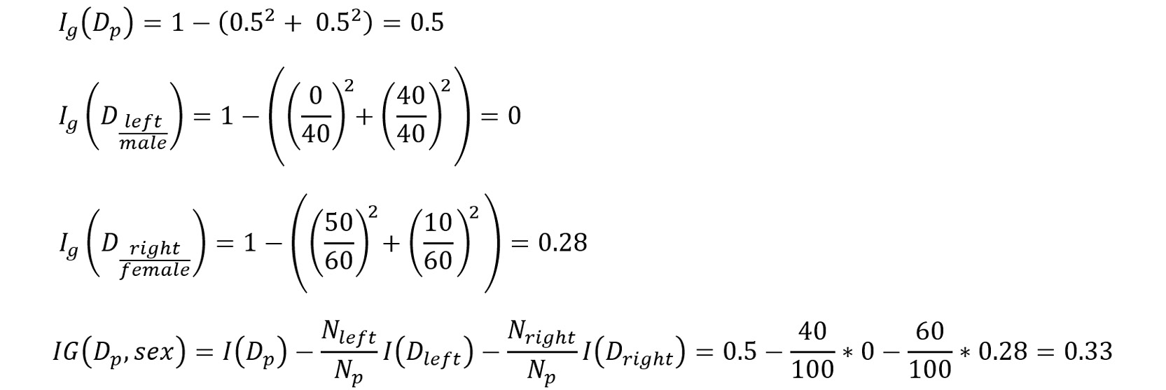
Figure 8.30: Information gain calculated using Gini impurity (Sex)

From the information gain calculated, the decision tree will split based on the Sex feature, for which the information gain value is 0.33.

Note

Similarly, information gain can be calculated using entropy and misclassification. You are encouraged to try these two calculations on your own.

So far, we have covered two popular classification algorithms – SVMs and decision tree classifiers. Now it's time to take things up a notch and discuss a very powerful classification algorithm – random forest. As the name suggests, random forest classifiers are nothing but a forest or a collection of decision trees. Let's go into more detail in the next section.

Random Forest

The decision tree algorithm that you saw earlier faced the problem of overfitting. Since you fit only one tree on the training data, there is a high chance that the tree will overfit the data without proper pruning. For example, referring to the Amazon sales case study that we discussed at the start of this chapter, if your model learns to focus on the inherent randomness in the data, it will try to use that as a baseline for future predictions. Consider a scenario where out of 100 customers, 90 bought a beard wash, primarily because most of them were males with a beard.

However, your model started thinking that this is not related to gender, so the next time someone logs in during the sale, it will start recommending beard wash, even if that person might be female. Unfortunately, these things are very common but can really harm the business. This is why it is important to treat the overfitting of models. The random forest algorithm reduces variance/overfitting by averaging multiple decision trees, which individually suffer from high variance.

Random forest is an ensemble method of supervised machine learning. Ensemble methods combine predictions obtained from multiple base estimators/classifiers to improve the robustness of the overall prediction. Ensemble methods are divided into the following two types:

• Bagging: The data is randomly divided into several subsets and the model is trained over each of these subsets. Several estimators are built independently from each other and then the predictions are averaged together, which ultimately helps to reduce variance (overfitting). Random forests belong to this category.
• Boosting: In the case of boosting, base estimators are built sequentially and each model built is very weak. The objective, therefore, is to build models in sequence, where the latter models try to reduce the error from the previous model and thereby reduce bias (underfitting). Advanced machine learning algorithms like CatBoost and XGBoost belong to this category.

Let's understand how the random forest algorithm works with the help of Figure 8.31:

1. A random bootstrap sample (a sample drawn with replacement) of size m is chosen from the training data. This splits the training data into subsets such as Data1, Data2, and so on.
2. Decision trees are grown on each instance of the bootstrap. These decision trees can be referred to as Learner1, Learner2, and so on.
3. d features are chosen randomly without replacement.
4. Each node is split using the d features selected based on objective functions, which could be information gain.
5. Steps 1-4 are repeated k times. Eventually, this generates Model1, Model2, and so on for each subset.
6. All of the predictions from the multiple trees are aggregated and assigned a class label by majority vote. This step is referred to as Model Combiner in Figure 8.31:

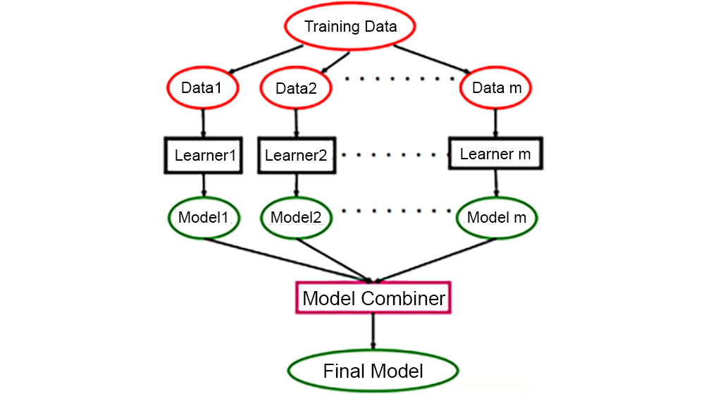
Figure 8.31: The working of a random forest model

The following are the advantages and disadvantages of the random forest algorithm:

Advantages

• It does not suffer from overfitting, since you take the average of all the predictions.
• It can be used to get feature importance.
• It can be used for both regression and classification tasks.
• It can be used for highly imbalanced datasets.
• It can handle missing data.

Disadvantages

• It suffers from bias, although it reduces variance.
• It's mostly a black-box model and is difficult to explain.

Similar to the decision tree algorithm, you can implement a random forest classifier using the scikit-learn module as follows:

1. Import RandomForestClassifier from scikit-learn:

   from sklearn.ensemble import RandomForestClassifier

2. Create an instance of the random forest classifier. You can specify the number of trees (n_estimators), the maximum depth of the trees, a random state (to add reproducibility to the results), and so on. A complete list of parameters can be found at https://scikit-learn.org/stable/modules/generated/sklearn.ensemble.RandomForestClassifier.html.

   clf = RandomForestClassifier(n_estimators=20, max_depth=None,

                               min_samples_split=7,

                               random_state=0)

3. Next, you can fit the classifier on the training dataset using clf.fit(X_train,y_train) and use it for prediction on input data using clf.predict(X).

Now that we have discussed the implementation of random forests using scikit-learn, let's train a random forest model on the Shill Bidding dataset and see how it compares to the accuracies obtained from the other classifiers we have trained so far.

Exercise 8.03: Implementing a Random Forest Model over a Dataset

In this exercise, you will use a random forest to build a model over the same auction dataset used previously. Ensure that you use the same Jupyter notebook as the one used for the preceding exercise:

1. Import the random forest classifier:

   from sklearn.ensemble import RandomForestClassifier

2. Fit the random forest classifier to the training data using the following code:

   clf = RandomForestClassifier(n_estimators=20, max_depth=None,

                               min_samples_split=7, random_state=0)

   clf.fit(X_train,y_train)

   You will get the following output by running the preceding code. Please note the output may vary on your system.

   RandomForestClassifier(min_samples_split=7, n_estimators=20, random_state=0)

3. Calculate the accuracy score:

   clf.score(X_test, y_test)

   You should get an output close to 0.9896, which means that the random forest classifier scores an accuracy of around 99%.

Now that you have implemented all three classical algorithms on the same dataset, let's do a quick comparison of their accuracies.

Classical Algorithms – Accuracy Compared

In the previous sections, we covered the mathematics behind each algorithm and learned about their advantages and their disadvantages. Through three exercises, you implemented each algorithm on the same dataset. In Figure 8.32, you can see a summary of the accuracy percentages you got. Circling back to the Amazon case study we discussed at the start of the chapter, it is clear that you would choose the decision tree classifier to predict whether a customer will buy a product during sales:

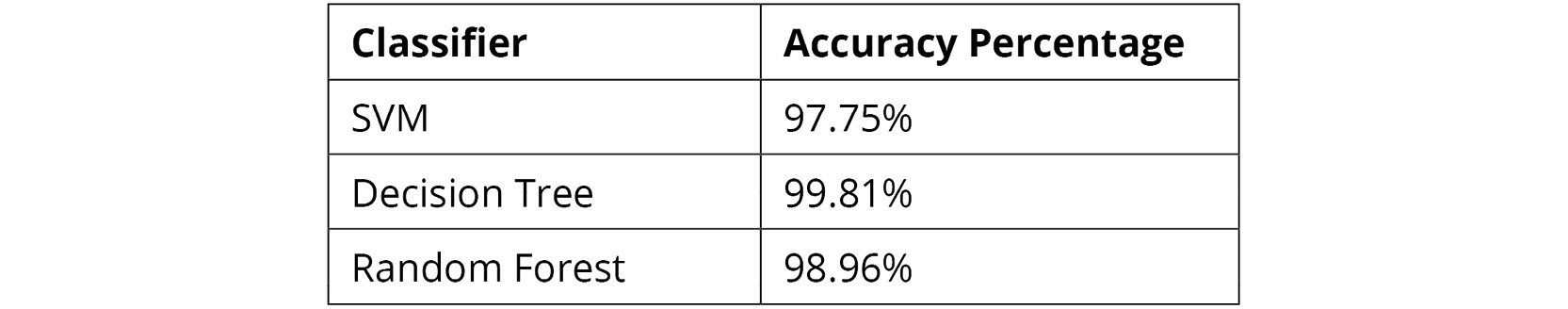
Figure 8.32: Accuracy percentages compared

Let's test the skills you have learned so far to perform an activity where you will implement all the algorithms you have learned so far. Later, you will learn why accuracy is not necessarily the only factor in choosing the model.

Activity 8.01: Implementing Different Classification Algorithms

In this activity, you will continue working with the telecom dataset (Telco_Churn_Data.csv) that you used in the previous chapter and will build different models from this dataset using the scikit-learn API. Your marketing team was impressed with the initial findings, and they now want you to build a machine learning model that can predict customer churn. This model will be used by the marketing team to send out discount coupons to customers who may churn. To build the best prediction model, it is important to try different algorithms and come up with the best-performing algorithm for the marketing team to use. In this activity, you will use the logistic regression, SVM, and random forest algorithms and compare the accuracies obtained from the three classifiers.

Note

In Activity 7.02, Performing MN of OSEMN, you saved the seven most important features to the top7_features variable. You will use these features to build our machine learning model. Please continue from the Activity8.01_starter.ipynb notebook present at https://packt.link/buxSG to implement the steps given in the following section.

Follow these steps:

1. Import the libraries for the logistic regression, decision tree, SVM, and random forest algorithms.
2. Fit individual models to the clf_logistic, clf_svm, clf_decision, and clf_random variables.

   Use the following parameters to ensure your results are more or less close to ours: for the logistic regression model, use random_state=0 and solver='lbfgs'; for the SVM, use kernel='linear' and C=1; and for the random forest model, use n_estimators=20, max_depth=None, min_samples_split=7, and random_state=0.

3. Use the score function to get the accuracy for each of the algorithms.

You should get accuracy scores similar to the ones listed in the following figure for each of the models at the end of this activity:

Figure 8.33: Comparison of different algorithm accuracies on the telecom dataset

Note

The solution to this activity can be found via this link.

Preprocessing Data for Machine Learning Models

Preprocessing data before training any machine learning model can improve the accuracy of the model to a large extent. Therefore, it is important to preprocess data before training a machine learning algorithm on the dataset. Preprocessing data consists of the following methods: standardization, scaling, and normalization. Let's look at these methods one by one.

Standardization

Most machine learning algorithms assume that all features are centered at zero and have variance in the same order. In the case of linear models such as logistic and linear regression, some of the parameters used in the objective function assume that all the features are centered around zero and have unit variance. If the values of a feature are much higher than some of the other features, then that feature might dominate the objective function and the estimator may not be able to learn from other features. In such cases, standardization can be used to rescale features such that they have a mean of 0 and a variance of 1. The following formula is used for standardization:

Figure 8.34: Standardization

Here, xi is the input data, µx is the mean, and σx is the standard deviation. Standardization is most useful for optimization algorithms such as gradient descent. The scikit-learn API has the StandardScalar utility class. Let's see how you can standardize the data using the StandardScalar utility class in the next exercise, where you will use the churn prediction data used in Chapter 7, Supervised Learning: Predicting Customer Churn. We provide the following sample implementation using the StandardScalar utility class:

1. Import the preprocessing library from scikit-learn. This has the StandardScalar utility class' implementation:

   from sklearn import preprocessing

2. Next, fit the scaler on a set of values – these values are typically the attributes of the training dataset:

   scaler = preprocessing.StandardScaler().fit(X_train)

3. Once you have the scaler ready, you can use it to transform both the training and test dataset attributes:

   X_train_scalar=scaler.transform(X_train)

   X_test_scalar=scaler.transform(X_test)

Now, you will use these same steps for standardizing the data in the bank churn prediction problem in the next exercise.

Exercise 8.04: Standardizing Data

For this exercise, you will use the bank churn prediction data that was used in Chapter 7, Supervised Learning: Predicting Customer Churn. In the previous chapter, you performed feature selection using a random forest. The features selected for your bank churn prediction data are Age, EstimatedSalary, CreditScore, Balance, and NumOfProducts.

In this exercise, your objective will be to standardize the data after you have carried out feature selection. On exploring the previous chapter, it was clear that data is not standardized; therefore in this exercise, you will implement StandardScalar to standardize the data to zero mean and unit variance. Ensure that you use the same notebook as the one used for the preceding two exercises. You can copy the notebook from this link: https://packt.link/R0vtb:

1. Import the preprocessing library:

   from sklearn import preprocessing

2. View the first five rows, which have the Age, EstimatedSalary, CreditScore, Balance, and NumOfProducts features:

   X_train[top5_features].head()

   You will get the following output:

   

   Figure 8.35: First few rows of top5_features

3. Fit the StandardScalar function on the X_train data using the following code:

   scaler = preprocessing.StandardScaler()

                         .fit(X_train[top5_features])

4. Check the mean and scaled values. Use the following code to show the mean values of the five columns:

   scaler.mean_

   You should get the following output:

   array([3.89098824e+01, 1.00183902e+05, 6.49955882e+02, 7.61412119e+04, 1.52882353e+00])

5. Now check the scaled values:

   scaler.scale_

   You should get the following output:

   array([1.03706201e+01, 5.74453373e+04, 9.64815072e+01, 6.24292333e+04, 5.80460085e-01])

   The preceding output shows the scaled values of the five columns. You can notice that the mean values have reduced slightly, making the entire dataset a better scaled-down version of the entire dataset.

   Note

   You can read more about the preceding two functions at https://scikit-learn.org/stable/modules/generated/sklearn.preprocessing.StandardScaler.html.

6. Apply the transform function to the X_train data. This function performs standardization by centering and scaling the training data:

   X_train_scalar=scaler.transform(X_train[top5_features])

7. Next, apply the transform function to the X_test data and check the output:

   X_test_scalar=scaler.transform(X_test[top5_features])

   X_train_scalar

   You will get the following output on checking the scalar transform data:

   

Figure 8.36: Scalar transformed data

As you can notice in the preceding output, the values have now been changed after standardization. It's also important to note here that just by seeing the values, no significant inference can be made after standardization. In the next section, you will go over another method of data preprocessing, scaling, where you will see the values getting scaled to a specific range.

Scaling

Scaling is another method for preprocessing your data. Scaling your data cause the features to lie between a certain minimum and maximum value, mostly between zero and one. As a result, the maximum absolute value of each feature is scaled.

It's important to point out here that StandardScaler focuses on scaling down the standard deviation of the dataset to 1, and that's why the effect on the mean is not significant. However, scaling focuses on bringing down the values directly to a given range – mostly from 0 to 1.

Scaling can be effective for the machine learning algorithms that use the Euclidean distance, such as K-Nearest Neighbors (KNN) or k-means clustering:

Figure 8.37: Equation for scaling data

Here, xi is the input data, xmin is the minimum value of the feature, and xmax is the maximum value of the feature. In scikit-learn, you use MinMaxScaler or MaxAbsScaler for scaling the data. Let's quickly see how to implement this using scikit-learn:

1. Import the preprocessing library from scikit-learn. This has the MinMaxScaler utility's implementation:

   from sklearn import preprocessing

2. Similar to the usage of StandardScaler, you will fit the scaler on training attributes:

   scaler = preprocessing.MinMaxScaler().fit(X_train)

3. Once you have the scaler ready, you can use it to transform both the training and test datasets' attributes:

   X_train_scalar=scaler.transform(X_train)

   X_test_scalar=scaler.transform(X_test)

Now, you can use these same steps to scale the data in the bank churn prediction problem in the exercise that follows.

Note

You can read more about the MinMaxScaler and MaxAbsScaler at https://scikit-learn.org/stable/modules/generated/sklearn.preprocessing.MinMaxScaler.html and https://scikit-learn.org/stable/modules/generated/sklearn.preprocessing.MaxAbsScaler.html.

Exercise 8.05: Scaling Data After Feature Selection

In this exercise, your objective is to scale data after feature selection. You will use the same bank churn prediction data to perform scaling. Ensure that you continue using the same Jupyter notebook. You can refer to Figure 8.35 to examine the top five features:

1. Fit the min_max scaler on the training data:

   min_max = preprocessing.MinMaxScaler().fit(X_train[top5_features])

2. Check the minimum and scaled values:

   min_max.min_

   You will get the following mean values:

   array([-2.43243243e-01, -5.79055300e-05, -7.00000000e-01,

   0.00000000e+00, -3.33333333e-01])

   Notice that MinMaxScaler has forced the dataset to change the minimum value to 0. This is because, by default, MinMaxScaler scales down the values to a range of 0 to 1. As pointed out earlier, StandardScaler changes the standard deviation, whereas MinMaxScaler directly changes the values with the intent of changing the upper and lower bounds of the dataset.

3. Now check the scaled values:

   min_max.scale_

   You will get the following scaled values:

   array([1.35135135e-02, 5.00047755e-06, 2.00000000e-03, 3.98568200e-06, 3.33333333e-01])

4. Transform the train and test data using min_max:

   X_train_min_max=min_max.transform(X_train[top5_features])

   X_test_min_max=min_max.transform(X_test[top5_features])

In this exercise, you saw how to perform scaling using the scikit-learn module's MinMaxScaler. Next, you will learn about the third method of data preprocessing – normalization.

Normalization

In normalization, individual training samples are scaled to have a unit norm. (The norm of a vector is the size or length of the vector. Hence, each of the training samples' vector lengths will be scaled to 1.) This method is mostly used when you want to use a quadratic form such as the dot product or any kernel to quantify sample similarity. It is most effective in clustering and text classification.

You use either the L1 norm or the L2 norm for normalization. The L1 norm is used to find the sum of the "magnitudes" of vectors, that's why you have the "absolute" part there in the equation. The L2 norm, on the other hand, finds the sum of the squares of values and then takes the square root to calculate the norm of the vector.

In general, the L2 norm is preferred simply because it's much faster compared to the L1 norm because of the implementation:

Figure 8.38: Normalization

xi is the input training samples.

Note

In scikit-learn, you use the Normalize and Normalizer utility classes. The difference between the two normalizations is out of the scope of this chapter.

You can use the Normalizer class in scikit-learn as follows:

1. Import the preprocessing library from scikit-learn. This has the Normalizer utility's implementation:

   from sklearn import preprocessing

2. Similar to the usage of StandardScaler, you will fit the Normalizer class on the training attributes:

   normalize = preprocessing.Normalizer().fit(X_train)

3. Once you have the Normalizer ready, you can use it to transform both the training and test dataset attributes:

   X_train_normalize=normalize.transform(X_train)

   X_test_normalize=normalize.transform(X_test)

Now that you have covered the theory of normalization, let's use the utility functions available in scikit-learn to perform normalization in the next exercise.

Exercise 8.06: Performing Normalization on Data

In this exercise, you are required to normalize data after feature selection. You will use the same bank churn prediction data for normalizing. Continue using the same Jupyter notebook as the one used in the preceding exercise:

1. Fit the Normalizer() on the training data:

   normalize = preprocessing.Normalizer()

                            .fit(X_train[top5_features])

2. Check the normalize function:

   normalize

   This will give you the following output:

   Normalizer()

3. Transform the training and testing data using normalize:

   X_train_normalize=normalize.transform(X_train[top5_features])

   X_test_normalize=normalize.transform(X_test[top5_features])

   You can verify that the norm has now changed to 1 using the following code:

   np.sqrt(np.sum(X_train_normalize**2, axis=1))

   This gives the following output:

   array([1., 1., 1., ..., 1., 1., 1.])

4. Similarly, you can also evaluate the norm of the normalized test dataset:

   np.sqrt(np.sum(X_test_normalize**2, axis=1))

   This gives the following output:

   array([1., 1., 1., ..., 1., 1., 1.])

In the preceding exercise, you carried out data normalization using an L2-norm-based Normalizer. That completes the implementation of the three data preprocessing techniques. It's also important to note here that you do not need to perform all three preprocessing techniques; any one of the three methods would suffice. While these methods are carried out before feeding the data to a model for training, you will next discuss the methods for evaluating the model once it has been trained. This will help in choosing the best model out of a given set of models.

Model Evaluation

When you train your model, you usually split the data into training and testing datasets. This is to ensure that the model doesn't overfit. Overfitting refers to a phenomenon where a model performs very well on the training data but fails to give good results on testing data, or in other words, the model fails to generalize.

In scikit-learn, you have a function known as train_test_split that splits the data into training and testing sets randomly.

When evaluating your model, you start by changing the parameters to improve the accuracy as per your test data. There is a high chance of leaking some of the information from the testing set into your training set if you optimize your parameters using only the testing set data. To avoid this, you can split data into three parts—training, testing, and validation sets. However, the disadvantage of this technique is that you will be further reducing your training dataset.

The solution is to use cross-validation. In this process, you do not need a separate validation dataset; instead, you split your dataset into training and testing data. However, the training data is split into k smaller sets using a technique called k-fold cross-validation, which can be explained using the following figure:

Figure 8.39: K-fold cross-validation

The algorithm is as follows. Assume k=10; that is, you will have 10 folds, as shown in the preceding figure:

1. The entire training data is divided into k folds, in this case, it's 10. In the preceding figure, you can see all the 10 folds, and each fold having 10 separations of the dataset.
2. The model is trained on k-1 portions (white blocks highlighted in the preceding figure, with the black blocks signifying the untrained portion). In this case, you will be training the model on 9 different portions in each fold. You can notice that the black blocks are at different positions in each of the 10 folds, thus signifying that different portions are being trained in each fold.
3. Once the model is trained, the classifier is evaluated on the remaining 1 portion (black blocks highlighted in the preceding figure).

   Steps 2 and 3 are repeated k times. This is why you have 10 folds in the preceding figure.

4. Once the classifier has carried out the evaluation, an overall average score is taken.

This method doesn't work well if you have a class imbalance, and therefore you use a method known as stratified K fold.

Note

In many classification problems, you will find that classes are not equally distributed. One class may be highly represented, that is, 90%, while another class may consist of only 10% of the samples. For example, when dealing with a dataset containing information about the products purchased on an e-commerce website to predict whether a purchase will be returned or not, the percentage of returned orders will be significantly smaller than the non-returned ones. We will cover how to deal with imbalanced datasets in the next chapter.

You use stratified k-fold to deal with datasets where there is a class imbalance. In datasets where there is a class imbalance, during splitting, care must be taken to maintain class proportions. In the case of stratified k-fold, it maintains the ratio of classes in each portion.

In order to implement stratified k-fold cross-validation, use the following steps:

1. Import StratifiedKFold from the scikit-learn module:

   from sklearn.model_selection import StratifiedKFold

2. Create a StratifiedKFold instance. You can choose the value of the number of splits you want to make (k) and set a random state to make the results reproducible:

   skf = StratifiedKFold(n_splits=10,random_state=1)

3. Next, use the instance created in step 2 to split the X and y values:

   skf.split(X,y)

Now that we have discussed the details of cross-validation, stratified k-fold cross-validation, and its implementation, let's apply it to the bank churn prediction dataset in the next exercise.

Exercise 8.07: Stratified K-fold

In this exercise, you will fit the stratified k-fold function of scikit-learn to the bank churn prediction data and use the logistic regression classifier from the previous exercise to fit our k-fold data. Along with that, you will also implement the scikit-learn k-fold cross-validation scorer function:

Note

Please continue using the same notebook as the one used for the preceding exercise.

1. Import StratifiedKFold from sklearn:

   from sklearn.model_selection import StratifiedKFold

2. Fit the classifier on the training and testing data with n_splits=10:

   skf = StratifiedKFold(n_splits=10)

         .split(X_train[top5_features].values,y_train.values)

3. Calculate the k-cross fold validation score:

   results=[]

   for i, (train,test) in enumerate(skf):

       clf.fit(X_train[top5_features].values[train],

              y_train.values[train])

       fit_result=clf.score(X_train[top5_features].values[test],

                           y_train.values[test])

       results.append(fit_result)

       print('k-fold: %2d, Class Ratio: %s, Accuracy: %.4f'

             % (i,np.bincount(y_train.values[train]),fit_result))

   You will get the following result:

   

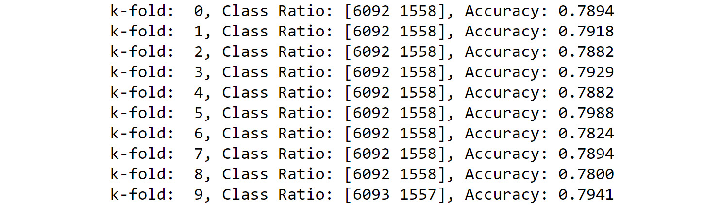
   Figure 8.40: Calculate the k-cross fold validation score

   You can see that the class ratio has stayed constant across all the k-folds.

4. Find the accuracy:

   print('accuracy for CV is:%.3f' % np.mean(results))

   You will get an output showing an accuracy close to 0.790.

5. Import the scikit-learn cross_val_score function:

   from sklearn.model_selection import cross_val_score

6. Fit the classifier and print the accuracy:

   results_cross_val_score=cross_val_score

                           (estimator=clf,

                            X=X_train[top5_features].values,

                            y=y_train.values,cv=10,n_jobs=1)

   print('accuracy for CV is:%.3f '

         % np.mean(results_cross_val_score))

   You will get an output showing the accuracy as 0.790. Even though both the accuracies are the same, it is still recommended to use stratified k-fold validation when there is a class imbalance.

In this exercise, you implemented k-fold cross-validation using two methods, one where you used a for loop and another where you used the cross_val_score function of sklearn. You used logistic regression as your base classifier present in the clf variable from Exercise 7.08, Building a Logistic Regression Model, in Chapter 7, Supervised Learning: Predicting Customer Churn. From the cross-validation, your logistic regression gave an accuracy of around 79% overall.

In this section, we covered an important aspect of model evaluation. You can use the same concept to make your models better by tweaking the hyperparameters that define the model. In the next section, you will go over this concept, which is also referred to as fine-tuning.

Fine-Tuning of the Model

In the case of a machine learning model, there are two types of parameter tuning that can be performed:

• The first one includes the parameters that the model uses to learn from itself, such as the coefficients in the case of linear regression or the margin in the case of SVM.
• The second one includes parameters that must be optimized separately. These are known as hyperparameters, for example, the alpha value in the case of lasso linear regression or the number of leaf nodes in the case of decision trees. In the case of a machine learning model, there can be several hypermeters and hence it becomes difficult for someone to tune the model by adjusting each of the hyperparameters manually. Consider a scenario where you have built a decision tree for predicting whether a given product will be returned by a customer or not. However, while building the model, you used the default values of the hyperparameters. You notice that you are obtaining a mediocre accuracy of 75%. While you can move on to the next classifier, for example, a random forest, it's important to first make sure that you have got the best result you could using the same class of classifier (a decision tree in this case). This is because there is a limit to the different categories of classifiers you can build, and if you keep on going for default values, you won't always come up with the best results. Optimizing the model performance by changing the hyperparameters helps in getting the best results from the classifier you are working on and thus gives you a better sample space of models to choose the best model from.

There are two methods for performing hypermeter search operations in scikit-learn, which are described as follows:

• Grid search: Grid search uses a brute-force exhaustive search to permute all combinations of hyperparameters, which are provided to it as a list of values.
• Randomized grid search: Randomized grid search is a faster alternative to grid search, which can be very slow due to the use of brute force. In this method, parameters are randomly chosen from a distribution that the user provides. Additionally, the user can provide a sampling iteration specified by n_iter, which is used as a computational budget.

In the cases of both grid search and randomized grid search, the implementation using scikit-learn stays more or less the same:

1. Import GridSearchCV and RandomizedSearchCV from the scikit-learn module:

   from sklearn.model_selection import GridSearchCV, RandomizedSearchCV

2. Specify the hyperparameters you want to run the search on:

   parameters = [ {'kernel': ['linear'], 'C':[0.1, 1, 10]},

                  {'kernel': ['rbf'], 'gamma':[0.5, 1, 2],

                   'C':[0.1, 1, 10]}]

3. Create instances of GridSearchCV and RandomizedSearchCV, specifying the estimator (classifier) to use and the list of hyperparameters. You can also choose to specify the method of cross-validation you want to use, for example with imbalanced data, you can go for StratifiedKFold cross-validation:

   clf = GridSearchCV(svm.SVC(), parameters)

   clf_random = RandomizedSearchCV(svm.SVC(), parameters)

4. Next, fit the preceding instances of grid search and randomized grid search on the training dataset:

   clf.fit(X_train,y_train)

   clf_random.fit(X_train,y_train)

5. You can then obtain the best score and the list of best hyperparameters, shown as follows:

   print(clf.best_score_, clf_random.best_score_)

   print(clf.best_params_, clf_random.best_params_)

In this section, we discussed the concept of fine-tuning a model using grid search and randomized grid search. You also saw how to implement both methods using the scikit-learn module. Now it's time to use these skills to fine-tune an SVM model on the bank churn prediction data you have been working on.

Exercise 8.08: Fine-Tuning a Model

In this exercise, you will implement a grid search to find out the best parameters for an SVM on the bank churn prediction data. You will continue using the same notebook as in the preceding exercise:

1. Import SVM, GridSearchCV, and StratifiedKfold:

   from sklearn import svm

   from sklearn.model_selection import GridSearchCV

   from sklearn.model_selection import StratifiedKFold

2. Specify the parameters for the grid search as follows:

   parameters = [{'kernel': ['linear'], 'C':[0.1, 1]},

                 {'kernel': ['rbf'], 'C':[0.1, 1]}]

3. Fit the grid search with StratifiedKFold, setting the parameter as n_splits = 3.

   Note

   Due to the large number of combinations of the parameters mentioned above, the model fitting can take up to 2 hours.

   clf = GridSearchCV(svm.SVC(), parameters,

                      cv = StratifiedKFold(n_splits = 3),

                      verbose=4,n_jobs=-1)

   clf.fit(X_train[top5_features], y_train)

   The preceding step gives the following output:

   

   Figure 8.41: Fitting the model

4. Print the best score and the best parameters:

   print('best score train:', clf.best_score_)

   print('best parameters train: ', clf.best_params_)

   You will get the following output:

   

Figure 8.42: The best score and parameters obtained from the grid search

Note

Grid search takes a lot of time to find out the optimum parameters, and hence, the search parameters given should be wisely chosen.

From this exercise, you can conclude that the best parameters chosen by the grid search were C:0.1, Gamma:0.5, and kernel:rbf

From the exercise, you saw how model tuning helps to achieve higher accuracy. Firstly, you implemented data preprocessing, which is the first step to improve the accuracy of a model. Later, you learned how cross-validation and grid search enable you to further tune the machine learning model and improve the accuracy. Now it's time for you to use these skills to fine-tune and optimize the random forest model you trained in Activity 8.01, Implementing Different Classification Algorithms.

Activity 8.02: Tuning and Optimizing the Model

The models you built in the previous activity produced good results, especially the random forest model, which produced an accuracy score of more than 80%. You now need to improve the accuracy of the random forest model and generalize it. Tuning the model using different preprocessing steps, cross-validation, and grid search will improve the accuracy of the model. You will be using the same Jupyter notebook as the one used in the preceding activity. Follow these steps:

1. Store five out of seven features, that is, Avg_Calls_Weekdays, Current_Bill_Amt, Avg_Calls, Account_Age, and Avg_Days_Delinquent, in a variable called top5_features. Store the other two features, Percent_Increase_MOM and Complaint_Code, in a variable called top2_features. These features have values in the range of −1 to 7, whereas the other five features have values in the range of 0 to 374457. Hence, you can leave these features and standardize the remaining five features.
2. Use StandardScalar to standardize the five features.
3. Create a variable called X_train_scalar_combined, and combine the standardized five features with the two features (Percent_Increase_MOM and Complaint_Code) that were not standardized.
4. Apply the same scalar standardization to the test data (X_test_scalar_combined).
5. Fit the random forest model.
6. Score the random forest model. You should get a value close to 0.81.
7. Import the library for grid search and use the following parameters:

   parameters = [ {'min_samples_split': [9,10],

                   'n_estimators':[100,150,160]

                   'max_depth': [5,7]}]

8. Use grid search cross-validation with stratified k-fold to find out the best parameters. Use StratifiedKFold(n_splits = 3) and RandomForestClassifier().
9. Print the best score and the best parameters. You should get the following values:

   Figure 8.43: Best score and best parameters

10. Score the model using the test data. You should get a score close to 0.824.

Combining the results of the accuracy score obtained in Activity 8.01, Implementing Different Classification Algorithms and Activity 8.02, Tuning and Optimizing the Model, here are the results for the random forest implementations:

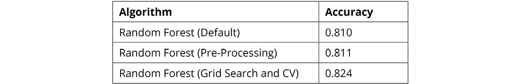
Figure 8.44: Comparing the accuracy of the random forest using different methods

You can conclude that data preprocessing and model-tuning methods can greatly improve model accuracy.

Note

The solution to this activity can be found via this link.

In the preceding sections, you have been using accuracy as the primary evaluation metric, however, there are several other performance metrics. The choice of correct evaluation metric (performance metric) is a very important decision one needs to make. Let's go over the various performance metrics you can use in the next section.

Performance Metrics

In the case of classification algorithms, we use a confusion matrix, which gives us the performance of the learning algorithm. It is a square matrix that counts the number of True Positive (TP), True Negative (TN), False Positive (FP), and False Negative (FN) outcomes:

Figure 8.45: Confusion matrix

For the sake of simplicity, let's use 1 as the positive class and 0 as a negative class, then:

TP: The number of cases that were observed and predicted as 1.

FN: The number of cases that were observed as 1 but predicted as 0.

FP: The number of cases that were observed as 0 but predicted as 1.

TN: The number of cases that were observed as 0 and predicted as 0.

Consider the same case study of predicting whether a product will be returned or not. In that case, the preceding metrics can be understood using the following table:

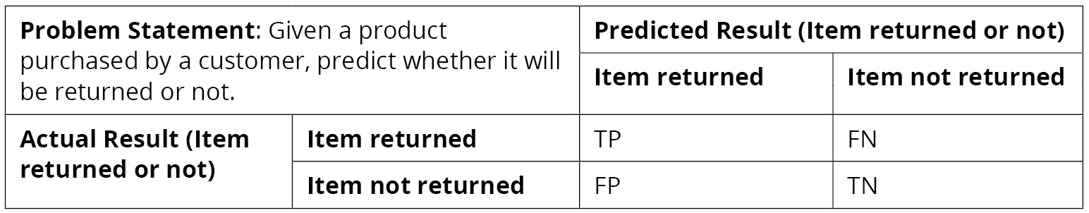
Figure 8.46: Understanding the metrics

Precision

Precision is the ability of a classifier to not label a sample that is negative as positive. The precision for an algorithm is calculated using the following formula:

Figure 8.47: Precision

This is useful in the case of email spam detection. In this scenario, you do not want any important emails to be detected as spam. In other words, you want to keep FPs as low as possible, even if it means recognizing some spam mails as not spam. In scenarios like these, precision is the recommended evaluation metric to use.

Similar to precision, there is another evaluation metric that is commonly used when you want to reduce FNs as much as possible. Let's go over this evaluation metric in the next section.

Recall

Recall refers to the ability of a classifier to correctly identify all the positive samples, that is, out of the total pool of positive findings (tp + fn), how many were correctly identified. This is also known as the True Positive Rate (TPR) or sensitivity and is given by the following formula:

Figure 8.48: Recall

This is useful in scenarios where, for example, you want to detect whether a customer will churn or not. In that scenario, you can use the recall score, since your main objective is to detect all the customers who will churn so that you can give them some exciting offers to make sure they stay with your company. Even if the classifier predicts a customer that was not going to leave the company as "churn," the customer will just get an offer for free, which is not a huge loss.

F1 Score

This is the harmonic mean of precision and recall. It is given by the following formula:

Figure 8.49: F1 score

F1 score can be useful when you want to have an optimal blend of precision and recall. For example, referring to the case study of predicting whether an item will be returned or not, imagine the company decides to offer some discount to make sure that an item is not returned (which would mean extra logistics expenses). If you mistakenly predict an item as prone to being returned, the company will have to give a discount even when it was not required, thereby causing a loss to the company. On the other hand, if you mistakenly predict an item as not to be returned, the company will have to suffer the logistics expenses, again causing a loss. In situations like this, the F1 score can come to the rescue as it takes into account both precision and recall.

You will also use the classification_report utility function present in the scikit-learn library. This report shows a tabular representation of precision, recall, accuracy, and F1 score and helps in summarizing the performance of the classifier. To implement it, follow these steps:

1. Import classification_report from scikit-learn's metrics module:

   from sklearn.metrics import classification_report

2. Next, you can print the classification report by passing the parameters shown as follows:

   print(classification_report(y_test, y_pred,

                              target_names=target_names))

   Here, y_test refers to the actual target values, y_pred refers to the predicted values, and target_names refers to the class names, for example, Churn and No Churn.

Now that you have gone through the three commonly used evaluation metrics, let's evaluate these metrics for the random forest model trained on the bank churn prediction dataset.

Exercise 8.09: Evaluating the Performance Metrics for a Model

In this exercise, you will calculate the F1 score and the accuracy of our random forest model for the bank churn prediction dataset. Continue using the same notebook as the one used in the preceding exercise:

1. Import RandomForestClassifier, metrics, classification_report, confusion matrix, and accuracy_score:

   from sklearn.ensemble import RandomForestClassifier

   from sklearn.metrics import classification_report,confusion_matrix,accuracy_score

   from sklearn import metrics

2. Fit the random forest classifier using the following code over the training data:

   clf_random = RandomForestClassifier(n_estimators=20,

                                      max_depth=None,

                                      min_samples_split=7,

                                      random_state=0)

   clf_random.fit(X_train[top5_features],y_train)

   This code will give the following output on execution:

   RandomForestClassifier(min_samples_split=7, n_estimators=20, random_state=0)

   Note

   The output may slightly vary on your system.

3. Predict on the test data the classifier:

   y_pred=clf_random.predict(X_test[top5_features])

4. Print the classification report:

   target_names = ['No Churn', 'Churn']

   print(classification_report(y_test, y_pred,

                              target_names=target_names))

   Your output will look as follows:

   

   Figure 8.50: Classification report

5. Fit the confusion matrix and save it into a pandas DataFrame named cm_df:

   cm = confusion_matrix(y_test, y_pred)

   cm_df = pd.DataFrame(cm,

                        index = ['No Churn','Churn'],

                        columns = ['No Churn','Churn'])

6. Plot the confusion matrix using the following code:

   plt.figure(figsize=(8,6))

   sns.heatmap(cm_df, annot=True,fmt='g',cmap='Greys_r')

   plt.title('Random Forest Accuracy:{0:.3f}'

             .format(accuracy_score(y_test, y_pred)))

   plt.ylabel('True Values')

   plt.xlabel('Predicted Values')

   plt.show()

   Note

   The value Greys_r (emboldened) is used to generate graphs in grayscale. You can also refer to the following document to get the code for the colored plot and the colored output: http://packt.link/NOjgT.

   You should get the following output:

   

Figure 8.51: Confusion matrix

From this exercise, you can conclude that the random forest model has an overall F1 score of 0.82 (refer to the classification report). However, the F1 score of the customers who have churned is less than 50%. This is due to highly imbalanced data, as a result of which the model fails to generalize. You will learn how to make the model more robust and improve the F1 score for imbalanced data in the next chapter.

ROC Curve

The Receiver Operating Characteristic (ROC) curve is a graphical method used to inspect the performance of binary classification models by shifting the decision threshold of the classifier. It is plotted based on the TPR (or recall) and the False Positivity Rate (FPR). You saw what the TPR is in the last section. The FPR is given by the following equation:

Figure 8.52: The FPR (1−specificity)

This is equivalent to 1−specificity.

Specificity is defined as −ve Recall.

Negative Recall is the ability of a classifier to correctly find all the negative samples, that is, out of the total pool of negatives (tn + fp), how many were correctly identified as negative. It is represented by the following equation:

Figure 8.53: −ve Recall

The following diagram illustrates how an ROC curve is plotted:

Figure 8.54: ROC curve

The diagonal of the ROC curve represents random guessing. Classifiers that lie below the diagonal are considered to perform worse than random guessing. A perfect classifier would have its ROC curve in the top left corner, having a TPR of 1 and an FPR of 0.

Now that we have discussed some new evaluation metrics, let's use them in the bank churn prediction dataset for plotting the ROC curve and getting the area under the ROC curve in the next exercise.

Exercise 8.10: Plotting the ROC Curve

In this exercise, you will plot the ROC curve for the random forest model from the previous exercise on the bank churn prediction data. Continue with the same Jupyter notebook as the one used in the preceding exercise:

1. Import roc_curve,auc:

   from sklearn.metrics import roc_curve,auc

2. Calculate the TPR, FPR, and threshold using the following code:

   fpr, tpr, thresholds = roc_curve(y_test, y_pred, pos_label=1)

   roc_auc = metrics.auc(fpr, tpr)

3. Plot the ROC curve using the following code:

   plt.figure()

   plt.title('Receiver Operating Characteristic')

   plt.plot(fpr, tpr, label='%s AUC = %0.2f' %

            ('Random Forest', roc_auc, color = 'gray'))

   plt.plot([0, 1], [0, 1],'k--')

   plt.xlim([0.0, 1.0])

   plt.ylim([0.0, 1.05])

   plt.ylabel('Sensitivity(True Positive Rate)')

   plt.xlabel('1-Specificity(False Positive Rate)')

   plt.title('Receiver Operating Characteristic')

   plt.legend(loc="lower right")

   plt.show()

   Note

   The gray value for the color attribute is used to generate the graph in grayscale. You can use values such as red, r, and so on as values for the color parameter to get the colored graphs. You can also refer to the following document to get the code for the colored plot and the colored output: http://packt.link/NOjgT.

   Your plot should appear as follows:

   

Figure 8.55: ROC curve

From our exercise, it can be concluded that the model has an area under the curve of 0.67. Even though the F1 score of the model was calculated to be 0.82, from our classification report, the AUC (Area Under Curve) score is much less. The FPR is closer to 0, however, the TPR is closer to 0.4. The AUC curve and the overall F1 score can be greatly improved by preprocessing the data and fine-tuning the model using techniques that you implemented in the previous exercise.

In Activity 8.02, Tuning and Optimizing the Model, you saw how using fine-tuning techniques greatly improved your model accuracy. In the final activity for this chapter, you will have to find out the performance of the random forest model and compare the ROC curves of all the models.

Activity 8.03: Comparison of the Models

In the previous activity, you improved the accuracy score of the random forest model score to 0.82. However, you were not using the correct performance metrics. In this activity, you will have to find out the F1 score of the random forest model trained in the previous activities and also compare the ROC curve of different machine learning models created in Activity 8.01, Implementing Different Classification Algorithms.

Ensure that you use the same Jupyter notebook as the one used in the preceding activity. Follow these steps:

1. Import the required libraries.
2. Fit the random forest classifier with the parameters obtained from grid search in the preceding activity. Use the clf_random_grid variable.
3. Predict on the standardized scalar test data, X_test_scalar_combined.
4. Fit the classification report. You should get the following output:

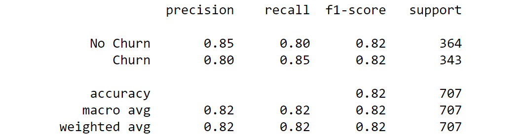
   Figure 8.56: Classification report

5. Plot the confusion matrix. Your output should be as follows:

   Figure 8.57: Confusion matrix

6. Import the library for the AUC and ROC curve.
7. Use the classifiers that were created in Activity 8.01, Implementing Different Classification Algorithms, that is, clf_logistic, clf_svm, clf_decision, and clf_random_grid. Create a dictionary of all these models.
8. Plot the ROC curve. The following for loop can be used as a hint:

   for m in models:

       model = m['model']

       ------ FIT THE MODEL

       ------ PREDICT

       ------ FIND THE FPR, TPR AND THRESHOLD

       roc_auc =FIND THE AUC

       plt.plot(fpr, tpr, label='%s AUC = %0.2f'

                % (m['label'], roc_auc))

   plt.plot([0, 1], [0, 1],'r--')

   plt.xlim([0.0, 1.0])

   plt.ylim([0.0, 1.05])

   plt.ylabel('Sensitivity(True Positive Rate)')

   plt.xlabel('1-Specificity(False Positive Rate)')

   plt.title('Receiver Operating Characteristic')

   plt.legend(loc="lower right")

   plt.show()

   You plot should look as follows:

   

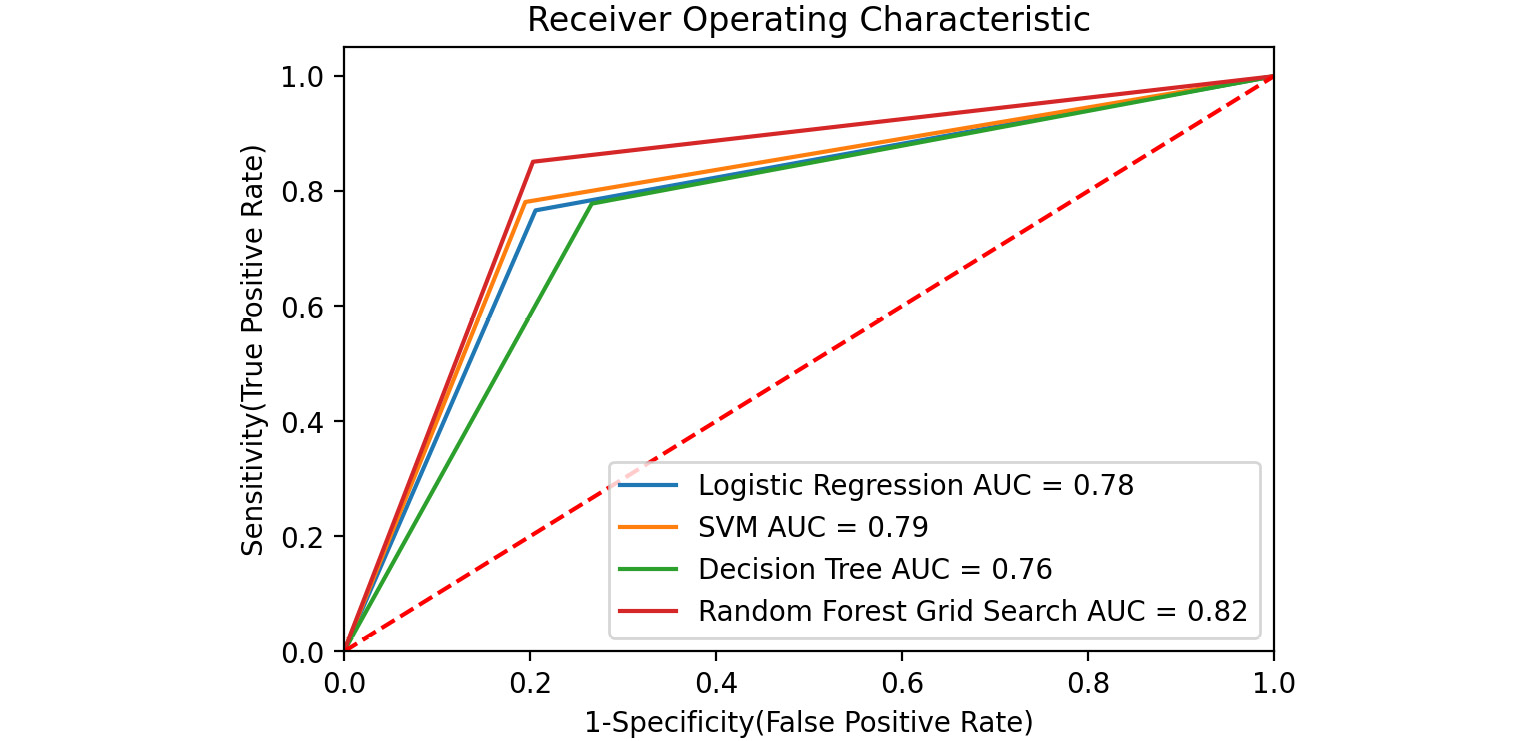
Figure 8.58: ROC curve

Note

The solution to this activity can be found via this link.

Summary

In this chapter, you learned how to perform classification using some of the most commonly used algorithms. After discovering how tree-based models work, you were able to calculate information gain, Gini values, and entropy. You applied these concepts to train decision tree and random forest models on two datasets.

Later in the chapter, you explored why the preprocessing of data using techniques such as standardization is necessary. You implemented various fine-tuning techniques for optimizing a machine learning model. Next, you identified the right performance metrics for your classification problems and visualized performance summaries using a confusion matrix. You also explored other evaluation metrics including precision, recall, F1 score, ROC curve, and the area under the curve.

You implemented these techniques on case studies such as the telecom dataset and customer churn prediction and discovered how similar approaches can be followed in predicting whether a customer will buy a product or not during a sales season.

In the next chapter, you will learn about multi-classification problems and how to tackle imbalanced data.