1. Data Preparation and Cleaning

Overview

In this chapter, you'll learn the skills required to process and clean data to effectively ready it for further analysis. Using the pandas library in Python, you will learn how to read and import data from various file formats, including JSON and CSV, into a DataFrame. You'll then learn how to perform slicing, aggregation, and filtering on DataFrames. By the end of the chapter, you will consolidate your data cleaning skills by learning how to join DataFrames, handle missing values, and even combine data from various sources.

Introduction

"Since you liked this artist, you'll also like their new album," "Customers who bought bread also bought butter," and "1,000 people near you have also ordered this item." Every day, recommendations like these influence customers' shopping decisions, helping them discover new products. Such recommendations are possible thanks to data science techniques that leverage data to create complex models, perform sophisticated tasks, and derive valuable customer insights with great precision. While the use of data science principles in marketing analytics is a proven, cost-effective, and efficient strategy, many companies are still not using these techniques to their full potential. There is a wide gap between the possible and actual usage of these techniques.

This book is designed to teach you skills that will help you contribute toward bridging that gap. It covers a wide range of useful techniques that will allow you to leverage everything data science can do in terms of strategies and decision-making in the marketing domain. By the end of the book, you should be able to successfully create and manage an end-to-end marketing analytics solution in Python, segment customers based on the data provided, predict their lifetime value, and model their decision-making behavior using data science techniques.

You will start your journey by first learning how to clean and prepare data. Raw data from external sources cannot be used directly; it needs to be analyzed, structured, and filtered before it can be used any further. In this chapter, you will learn how to manipulate rows and columns and apply transformations to data to ensure you have the right data with the right attributes. This is an essential skill in a data analyst's arsenal because, otherwise, the outcome of your analysis will be based on incorrect data, thereby making it a classic example of garbage in, garbage out. But before you start working with the data, it is important to understand its nature - in other words, the different types of data you'll be working with.

Data Models and Structured Data

When you build an analytical solution, the first thing that you need to do is to build a data model. A data model is an overview of the data sources that you will be using, their relationships with other data sources, where exactly the data from a specific source is going to be fetched, and in what form (such as an Excel file, a database, or a JSON from an internet source).

Note

Keep in mind that the data model evolves as data sources and processes change.

A data model can contain data of the following three types:

• Structured Data: Also known as completely structured or well-structured data, this is the simplest way to manage information. The data is arranged in a flat tabular form with the correct value corresponding to the correct attribute. There is a unique column, known as an index, for easy and quick access to the data, and there are no duplicate columns. For example, in Figure 1.1, employee_id is the unique column. Using the data in this column, you can run SQL queries and quickly access data at a specific row and column in the dataset easily. Furthermore, there are no empty rows, missing entries, or duplicate columns, thereby making this dataset quite easy to work with. What makes structured data most ubiquitous and easy to analyze is that it is stored in a standardized tabular format that makes adding, updating, deleting, and updating entries easy and programmable. With structured data, you may not have to put in much effort during the data preparation and cleaning stage.

  Data stored in relational databases such as MySQL, Amazon Redshift, and more are examples of structured data:

  

Figure 1.1: Data in a MySQL table

• Semi-structured data: You will not find semi-structured data to be stored in a strict, tabular hierarchy as you saw in Figure 1.1. However, it will still have its own hierarchies that group its elements and establish a relationship between them. For example, metadata of a song may include information about the cover art, the artist, song length, and even the lyrics. You can search for the artist's name and find the song you want. Such data does not have a fixed hierarchy mapping the unique column with rows in an expected format, and yet you can find the information you need.

  Another example of semi-structured data is a JSON file. JSON files are self-describing and can be understood easily. In Figure 1.2, you can see a JSON file that contains personally identifiable information of Jack Jones.

  Semi-structured data can be stored accurately in NoSQL databases.

  

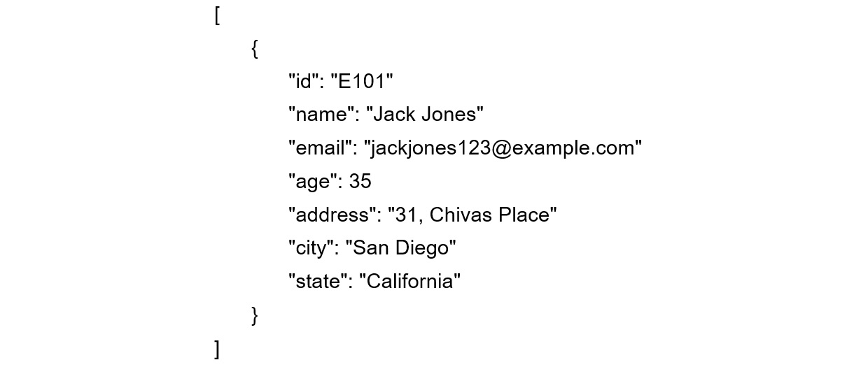
Figure 1.2: Data in a JSON file

• Unstructured data: Unstructured data may not be tabular, and even if it is tabular, the number of attributes or columns per observation may be completely arbitrary. The same data could be represented in different ways, and the attributes might not match each other, with values leaking into other parts.

  For example, think of reviews of various products stored in rows of an Excel sheet or a dump of the latest tweets of a company's Twitter profile. We can only search for specific keywords in that data, but we cannot store it in a relational database, nor will we be able to establish a concrete hierarchy between different elements or rows. Unstructured data can be stored as text files, CSV files, Excel files, images, and audio clips.

Marketing data, traditionally, comprises all three aforementioned data types. Initially, most data points originate from different data sources. This results in different implications, such as the values of a field could be of different lengths, the value for one field would not match that of other fields because of different field names, and some rows might have missing values for some of the fields.

You'll soon learn how to effectively tackle such problems with your data using Python. The following diagram illustrates what a data model for marketing analytics looks like. The data model comprises all kinds of data: structured data such as databases (top), semi-structured data such as JSON (middle), and unstructured data such as Excel files (bottom):

Figure 1.3: Data model for marketing analytics

As the data model becomes complex, the probability of having bad data increases. For example, a marketing analyst working with the demographic details of a customer can mistakenly read the age of the customer as a text string instead of a number (integer). In such situations, the analysis would go haywire as the analyst cannot perform any aggregation functions, such as finding the average age of a customer. These types of situations can be overcome by having a proper data quality check to ensure that the data chosen for further analysis is of the correct data type.

This is where programming languages such as Python come into play. Python is an all-purpose general programming language that integrates with almost every platform and helps automate data production and analysis.

Apart from understanding patterns and giving at least a basic structure to data, Python forces the data model to accept the right value for the attribute. The following diagram illustrates how most marketing analytics today structure different kinds of data by passing it through scripts to make it at least semi-structured:

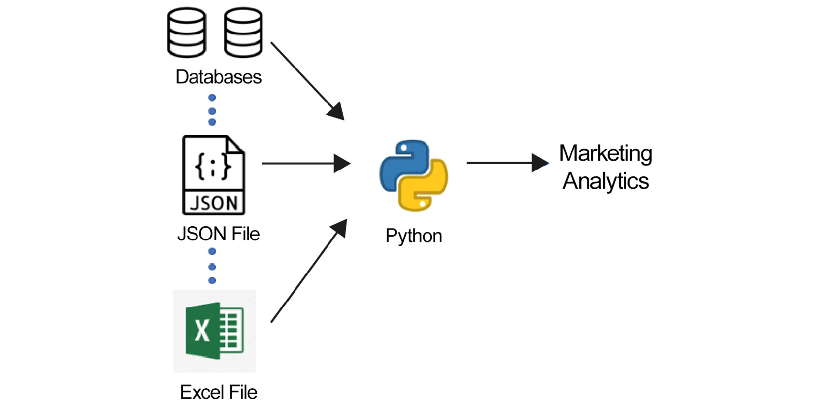
Figure 1.4: Data model of most marketing analytics that use Python

By making use of such structure-enforcing scripts, you will have a data model of semi-structured data coming in with expected values in the right fields; however, the data is not yet in the best possible format to perform analytics. If you can completely structure your data (that is, arrange it in flat tables, with the right value pointing to the right attribute with no nesting), it will be easy to see how every data point individually compares to other points with the help of common fields. You can easily get a feel of the data—that is, see in what range most values lie, identify the clear outliers, and so on—by simply scrolling through it.

While there are a lot of tools that can be used to convert data from an unstructured/semi-structured format to a fully structured format (for example, Spark, STATA, and SAS), the tool that is most widely used for data science, and which can be integrated with practically any framework, has rich functionalities, minimal costs, and is easy to use in our use case, is pandas.

pandas

pandas is a software library written in Python and is the basic building block for data manipulation and analysis. It offers a collection of high-performance, easy-to-use, and intuitive data structures and analysis tools that are of great use to marketing analysts and data scientists alike. The library comes as a default package when you install Anaconda (refer to the Preface for detailed instructions).

Note

Before you run the code in this book, it is recommended that you install and set up the virtual environment using the environment.yml file we have provided in the GitHub repository of this book.

You can find the environment.yml file at the following link: https://packt.link/dBv1k.

It will install all the required libraries and ensure that the version numbers of the libraries on your system match with ours. Refer to the Preface for more instructions on how to set this up.

However, if you're using any other distribution where pandas is not pre-installed, you can run the following command in your terminal app or command prompt to install the library:

pip install pandas

Note

On macOS or Linux, you will need to modify the preceding command to use pip3 instead of pip.

The following diagram illustrates how different kinds of data are converted to a structured format with the help of pandas:

Figure 1.5: Data model to structure the different kinds of data

When working with pandas, you'll be dealing with its two primary object types: DataFrames and Series. What follows is a brief explanation of what those object types are. Don't worry if you are not able to understand things such as their structure and how they work; you'll be learning more about these in detail later in the chapter.

• DataFrame: This is the fundamental tabular structure that stores data in rows and columns (like a spreadsheet). When performing data analysis, you can directly apply functions and operations to DataFrames.
• Series: This refers to a single column of the DataFrame. Series adds up to form a DataFrame. The values can be accessed through its index, which is assigned automatically while defining a DataFrame.

In the following diagram, the users column annotated by 2 is a series, and the viewers, views, users, and cost columns, along with the index, form a DataFrame (annotated by 1):

Figure 1.6: A sample pandas DataFrame and series

Now that you have a brief understanding of what pandas objects are, let's take a look at some of the functions you can use to import and export data in pandas.

Importing and Exporting Data with pandas DataFrames

Every team in a marketing group can have its own preferred data source for its specific use case. Teams that handle a lot of customer data, such as demographic details and purchase history, would prefer a database such as MySQL or Oracle, whereas teams that handle a lot of text might prefer JSON, CSV, or XML. Due to the use of multiple data sources, we end up having a wide variety of files. In such cases, the pandas library comes to our rescue as it provides a variety of APIs (Application Program Interfaces) that can be used to read multiple different types of data into a pandas DataFrame. Some of the most commonly used APIs are shown here:

Figure 1.7: Ways to import and export different types of data with pandas DataFrames

So, let's say you wanted to read a CSV file. You'll first need to import the pandas library as follows:

import pandas as pd

Then, you will run the following code to store the CSV file in a DataFrame named df (df is a variable):

df = pd.read_csv("sales.csv")

In the preceding line, we have sales.csv, which is the file to be imported. This command should work if your Jupyter notebook (or Python process) is run from the same directory where the file is stored. If the file was stored in any other path, you'll have to specify the exact path. On Windows, for example, you'll specify the path as follows:

df = pd.read_csv(r"C:UsersabhisDocumentssales.csv")

Note that we've added r before the path to take care of any special characters in the path. As you work with and import various data files in the exercises and activities in this book, we'll often remind you to pay attention to the path of the CSV file.

When loading data, pandas also provides additional parameters that you can pass to the read function, so that you can load the data the way you want. Some of these parameters are provided here. Please note that most of these parameters are optional. Also worth noting is the fact that the default value of the index in a DataFrame starts with 0:

• skiprows = k: This parameter skips the first k rows.
• nrows = k: This parameter parses only the first k rows.
• names = [col1, col2...]: This parameter lists the column names to be used in the parsed DataFrame.
• header = k: This parameter applies the column names corresponding to the kth row as the header for the DataFrame. k can also be None.
• index_col = col: This parameter sets col as the index of the DataFrame being used.

  index_col can also be a list of column names (used to create a MultiIndex) or it can be None. A MultiIndex DataFrame uses more than one column of the DataFrame as the index.

• usecols = [l1, l2...]: This provides either integer positional indices in the document columns or strings that correspond to column names in the DataFrame to be read; for example, [0, 1, 2] or ['foo', 'bar', 'baz'].

For example, if you want to import a CSV file into a DataFrame, df, with the following conditions:

• The first row of the file must be the header.
• You need to import only the first 100 rows into the file.
• You need to import only the first 3 columns.

The code corresponding to the preceding conditions would be as follows:

df= pd.read_csv("sales.csv",header=1,nrows=100,usecols=[0,1,2])

Note

There are similar specific parameters for almost every inbuilt function in pandas. You can find details about them with the documentation for pandas available at the following link: https://pandas.pydata.org/pandas-docs/stable/.

Once the data is imported, you need to verify whether it has been imported correctly. Let's understand how to do that in the following section.

Viewing and Inspecting Data in DataFrames

Once you've successfully read a DataFrame using the pandas library, you need to inspect the data to check whether the right attribute has received the right value. You can use several built-in pandas functions to do that.

The most commonly used way to inspect loaded data is using the head() command. By default, this command will display the first five rows of the DataFrame. Here's an example of the command used on a DataFrame called df:

df.head()

The output should be as follows:

Figure 1.8: Output of the df.head() command

Similarly, to display the last five rows, you can use the df.tail() command. Instead of the default five rows, you can even specify the number of rows you want to be displayed. For example, the df.head(11) command will display the first 11 rows.

Here's the complete usage of these two commands, along with a few other commands that be useful while examining data. Again, it is assumed that you have stored the DataFrame in a variable called df:

• df.head(n) will return the first n rows of the DataFrame. If no n is passed, the function considers n to be 5 by default.
• df.tail(n) will return the last n rows of the DataFrame. If no n is passed, the function considers n to be 5 by default.
• df.shape will return the dimensions of a DataFrame (number of rows and number of columns).
• df.dtypes will return the type of data in each column of the pandas DataFrame (such as float, object, int64, and so on).
• df.info() will summarize the DataFrame and print its size, type of values, and the count of non-null values.

So far, you've learned about the different functions that can be used on DataFrames. In the first exercise, you will practice using these functions to import a JSON file into a DataFrame and later, to inspect the data.

Exercise 1.01: Loading Data Stored in a JSON File

The tech team in your company has been testing a web version of its flagship shopping app. A few loyal users who volunteered to test the website were asked to submit their details via an online form. The form captured some useful details (such as age, income, and more) along with some not-so-useful ones (such as eye color). The tech team then tested their new profile page module, using which a few additional details were captured. All this data was stored in a JSON file called user_info.json, which the tech team sent to you for validation.

Note

You can find the user_info.json file at the following link: https://packt.link/Gi2O7.

Your goal is to import this JSON file into pandas and let the tech team know the answers to the following questions so that they can add more modules to the website:

• Is the data loading correctly?
• Are there any missing values in any of the columns?
• What are the data types of all the columns?
• How many rows and columns are present in the dataset?

  Note

  All the exercises and activities in this chapter can be performed in both the Jupyter notebook and Python shell. While you can do them in the shell for now, it is highly recommended to use the Jupyter notebook. To learn how to install Jupyter and set up the Jupyter notebook, refer to the Preface. It will be assumed that you are using a Jupyter notebook from this point on.

1. If you installed Anaconda as described in the Preface, a shortcut for Jupyter Notebook must have appeared on your system. Click it to launch Jupyter Notebook.
2. The Notebook Dashboard should appear in a new browser window (it opens in your default system browser) as follows:

   Figure 1.9: Notebook Dashboard

3. Using the Notebook Dashboard, navigate to the directory where you want to create your first Jupyter notebook. Click New. You'll see Python 3 along with several other options (as shown in Figure 1.10). If you've installed the virtual environment, you'll see ds-marketing as an option as well. Click ds-marketing if you're planning to use the virtual environment; otherwise, click Python 3. Either of these actions will open a new Jupyter notebook in a separate browser tab:

   Figure 1.10: Loading the YML environment

   Note

   To ensure that the version numbers of libraries we've used while writing this book match yours, make sure you install and use the ds-marketing virtual environment we have provided. Please refer to the Preface for detailed instructions.

4. Click the space that says Untitled in the header and rename the file as Exercise1.01. A .ipnyb extension will be added automatically:

   Figure 1.11: Renaming a file

5. In a new code cell, type in or paste the following command to import the pandas library. Use the Shift + Enter keyboard combination to execute the code:

   import pandas as pd

   Note

   You can find more information on what code cells are, what keyboard shortcuts to use, and what the structure of a notebook is, by visiting this guide in the official documentation: https://jupyter-notebook.readthedocs.io/en/stable/.

6. Create a new DataFrame called user_info and read the user_info.json file into it using the following command:

   user_info = pd.read_json("user_info.json")

   Note

   user_info.json should be stored in the same directory from which you are running Exercise1.01.ipnyb. Alternatively, you'll have to provide the exact path to the file as shown in the earlier Importing and Exporting Data with pandas DataFrames section.

7. Now, examine whether your data is properly loaded by checking the first five values in the DataFrame. Do this using the head() command:

   user_info.head()

   You should see the following output:

   

   Figure 1.12: Viewing the first few rows of user_info.json

   Note

   The preceding image does not contain all the columns of the DataFrame. It is used for demonstration purposes only.

   As you can see from the preceding screenshot, the data is successfully loaded into a pandas DataFrame. Therefore, you can now answer the first question with yes.

8. Now, to answer the second question, you'll need to use the info() command:

   user_info.info()

   You should get the following output:

   

   Figure 1.13: Information about the data in user_info

   Note

   The 64 displayed with the type above is an indicator of precision and varies on different platforms.

   From the preceding output, you can see that there are a total of 22 columns and 6 rows present in the JSON file. You may notice that the isActive column is a Boolean, the age and index columns are integers, and the latitude and longitude columns are floats. The rest of the columns are Python objects. Also, the number of observations in each column is the same (6), which implies that there are no missing values in the DataFrame. The preceding command not only gave us the answer to the second question, but it helped us answer the third and fourth questions as well. However, there is another quick way in which you can check the number of rows and columns in the DataFrame, and that is by using the shape attribute of the DataFrame.

9. Run the following command to check the number of rows and columns in the user_info DataFrame:

   user_info.shape

   This will give you (6, 22) as the output, indicating that the DataFrame created by the JSON has 6 rows and 22 columns.

In this exercise, you loaded the data, checked whether it had been loaded correctly, and gathered some more information about the entries contained therein. All this was done by loading data stored in a single source, which was the JSON file. As a marketing analyst, you will come across situations where you'll need to load and process data from different sources. Let's practice that in the exercise that follows.

Exercise 1.02: Loading Data from Multiple Sources

You work for a company that uses Facebook for its marketing campaigns. The data.csv file contains the views and likes of 100 different posts on Facebook used for a marketing campaign. The team also uses historical sales data to derive insights. The sales.csv file contains some historical sales data recorded in a CSV file relating to different customer purchases in stores in the past few years.

Your goal is to read the files into pandas DataFrames and check the following:

• Whether either of the datasets contains null or missing values
• Whether the data is stored in the correct columns and the corresponding column names make sense (in other words, the names of the columns correctly convey what type of information is stored in the rows)

  Note

  You can find the data.csv file at https://packt.link/NmBJT, and the sales.csv file at https://packt.link/ER7fz.

Let's first work with the data.csv file:

1. Start a new Jupyter notebook. You can name it Exercise 1.02. Then, import pandas by running the following command in a new Jupyter notebook cell. Use the Shift + Enter keyboard combination to run the code:

   import pandas as pd

2. Create a new DataFrame called campaign_data. Use the read_csv method to read the contents of the data.csv file into it:

   campaign_data = pd.read_csv("data.csv")

   Note

   Again, make sure that you're running the Jupyter notebook from the same directory where the data.csv file is stored. Otherwise, change the path (emboldened) as shown earlier in the Importing and Exporting Data with pandas DataFrames section.

3. Examine the first five rows of the DataFrame using the head() function:

   campaign_data.head()

   Your output should look as follows:

   

   Figure 1.14: Viewing raw campaign data

   From the preceding output, you can observe that views and likes appear as rows. Instead, they should be appearing as column names.

4. To read the column names, you will now read the data into campaign_data again (which is running the code in Step 2 once more), but this time you'll need to use the header parameter to make sure that the entries in the first row are read as column names. The header = 1 parameter reads the first row as the header:

   campaign_data = pd.read_csv("data.csv", header = 1)

   Run the head command again:

   campaign_data.head()

   You should get the following output:

   

   Figure 1.15: Output of the head command

   You will observe that views and likes are now displayed as column names.

5. Now, examine the last five rows using the tail() function:

   campaign_data.tail()

   You should get the following output:

   

   Figure 1.16: The last few rows of campaign_data

   There doesn't seem to be any misalignment of data or missing values toward the end of the DataFrame.

6. Although we have seen the last few rows, we still cannot be sure that all values in the middle (hidden) part of the DataFrame are devoid of any null values. Check the data types of the DataFrame to be sure using the following command:

   campaign_data.info()

   You should get the following output:

   

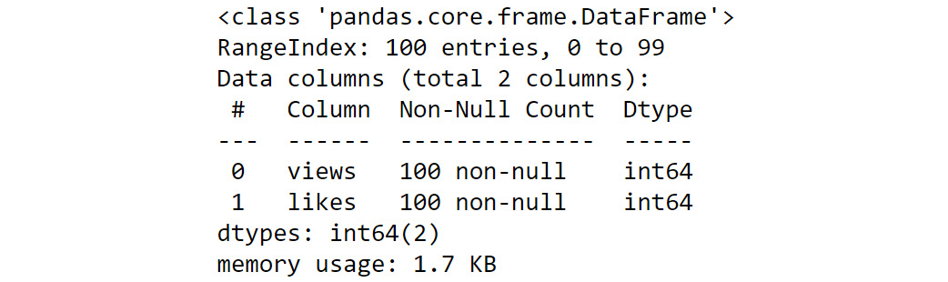
   Figure 1.17: info() of campaign_data

   As you can see from the preceding output, the DataFrame has two columns with 100 rows and has no null values.

7. Now, analyze the sales.csv file. Create a new DataFrame called sales. Use the read_csv() method to read the contents of the sales.csv file into it:

   sales = pd.read_csv("sales.csv")

   Note

   Make sure you change the path (emboldened) to the CSV file based on its location on your system. If you're running the Jupyter notebook from the same directory where the CSV file is stored, you can run the preceding code without any modification.

8. Look at the first five rows of the sales DataFrame using the following command:

   sales.head()

   Your output should look as follows:

   

   Figure 1.18: First few rows of sales.csv

   From the preceding screenshot, the Year column appears to have correct values, but the entries in the line column do not make sense. Upon closer examination, it's clear that the data that should have been loaded under a single column called Product line is split into two columns (Product and line). Thus, the first few products under this column should have read as Camping Equipment. The Product.1 and type columns suffer from a similar problem. Furthermore, the Order and method columns don't make much sense. In fact, the values of the Order and method columns being Water and Bag in one of the rows fail to convey any information regarding the data.

9. To check for null values and examine the data types of the columns, run the following command:

   sales.info()

   Your output should look as follows:

   

Figure 1.19: Output of sales.info()

From the preceding output, you can see that the country column has missing values (since all the other columns have 100 entries). You'll need to dig deeper and find out the exact cause of this problem. By the end of this chapter, you'll learn how to address such problems effectively.

Now that you have loaded the data and looked at the result, you can observe that the data collected by the marketing campaigns team (data.csv) looks good and it has no missing values. The data collected by the sales team, on the other hand (stored in sales.csv), has quite a few missing values and incorrect column names.

Based on what you've learned about pandas so far, you won't be able to standardize the data. Before you learn how to do that, you'll first have to dive deep into the internal structure of pandas objects and understand how data is stored in pandas.

Structure of a pandas DataFrame and Series

You are undecided as to which data structure to use to store some of the information that comes in from different marketing teams. From your experience, you know that a few elements in your data will have missing values. You are also expecting two different teams to collect the same data but categorize it differently. That is, instead of numerical indices (0-10), they might use custom labels to access specific values. pandas provides data structures that help store and work with such data. One such data structure is called a pandas series.

A pandas series is nothing more than an indexed NumPy array. To create a pandas series, all you need to do is create an array and give it an index. If you create a series without an index, it will create a default numeric index that starts from 0 and goes on for the length of the series, as shown in the following diagram:

Figure 1.20: Sample pandas series

Note

As a series is still a NumPy array, all functions that work on a NumPy array work the same way on a pandas series, too. To learn more about the functions, please refer to the following link:https://pandas.pydata.org/pandas-docs/stable/reference/series.html.

As your campaign grows, so does the number of series. With that, new requirements arise. Now, you want to be able to perform operations such as concatenation on specific entries in several series at once. However, to access the values, these different series must share the same index. And that's exactly where DataFrames come into the picture. A pandas DataFrame is just a dictionary with the column names as keys and values as different pandas series, joined together by the index.

A DataFrame is created when different columns (which are nothing but series) such as these are joined together by the index:

Figure 1.21: Series joined together by the same index create a pandas DataFrame

In the preceding screenshot, you'll see numbers 0-4 to the left of the age column. These are the indices. The age, balance, _id, about, and address columns, along with others, are series, and together they form a DataFrame.

This way of storing data makes it very easy to perform the operations you need on the data you want. You can easily choose the series you want to modify by picking a column and directly slicing off indices based on the value in that column. You can also group indices with similar values in one column together and see how the values change in other columns.

pandas also allows operations to be applied to both rows and columns of a DataFrame. You can choose which one to apply by specifying the axis, 0 referring to rows, and 1 referring to columns.

For example, if you wanted to apply the sum function to all the rows in the balance column of the DataFrame, you would use the following code:

df['balance'].sum(axis=0)

In the following screenshot, by specifying axis=0, you can apply a function (such as sum) on all the rows in a particular column:

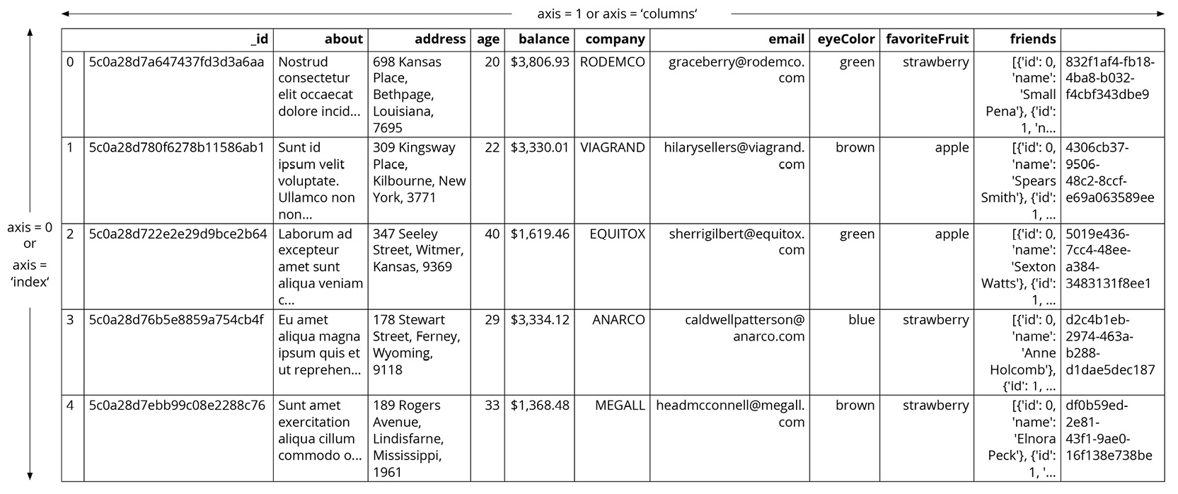
Figure 1.22: Understanding axis = 0 and axis = 1 in pandas

By specifying axis=1, you can apply a function on a row that spans across all the columns. In the next section, you will learn how to use pandas to manipulate raw data to gather useful insights from it.

Data Manipulation

Now that we have deconstructed the structure of the pandas DataFrame down to its basics, the remainder of the wrangling tasks, that is, creating new DataFrames, selecting or slicing a DataFrame into its parts, filtering DataFrames for some values, joining different DataFrames, and so on, will become very intuitive. Let's start by selecting and filtering in the following section.

Note

Jupyter notebooks for the code examples listed in this chapter can be found at the following links: https://packt.link/xTvR2 and https://packt.link/PGIzK.

Selecting and Filtering in pandas

If you wanted to access a particular cell in a spreadsheet, you would do so by addressing that cell in the familiar format of (column name, row name). For example, when you call cell A63, A refers to the column and 63 refers to the row. Data is stored similarly in pandas, but as (row name, column name) and we can use the same convention to access cells in a DataFrame.

For example, look at the following DataFrame. The viewers column is the index of the DataFrame:

Figure 1.23: Sample DataFrame

To find the cost of acquisition of Adam and Anurag along with their views, we can use the following code. Here, Adam and Anurag are the rows, and cost, along with views, are the columns:

df.loc[['Adam','Anurag'],['cost','views']]

Running the preceding command will generate the following output:

Figure 1.24: Use of the loc function

If you need to access more than a single cell, such as a subset of some rows and columns from the DataFrame, or change the order of display of some columns on the DataFrame, you can make use of the syntax listed in the following table:

Figure 1.25: A table listing the syntax used for different operations on a pandas DataFrame

In the next section, you'll learn how to create DataFrames in Python.

Creating DataFrames in Python

Let's say you've loaded campaign data into a DataFrame. In the revenue column, you see that the figures are not in their desired currencies. To convert the revenue numbers to various other currencies, you may need to create a test DataFrame, containing exchange rates that will remain constant throughout your revenue calculation.

There are two ways of creating such test DataFrames—by creating completely new DataFrames, or by duplicating or taking a slice of a previously existing DataFrame:

• Creating new DataFrames: You typically use the DataFrame function to create a completely new DataFrame. The function directly converts a Python object into a pandas DataFrame. The DataFrame function in general works with any iterable collection of data, such as dict and list. You can also pass an empty collection or a singleton collection to it.

  For example, you will get the same DataFrame through either of the following lines of code:

  df=pd.DataFrame({'Currency': pd.Series(['USD','EUR','GBP']),

                   'ValueInINR': pd.Series([70, 89, 99])})

  df=pd.DataFrame.from_dict({'Currency': ['USD','EUR','GBP'],

                             'ValueInINR':[70, 89, 99]})

  df.head()

  Running the command in either of these two ways will generate the following output:

  

Figure 1.26: Output generated by two different ways to create a DataFrame

• Duplicating or slicing a previously existing DataFrame: The second way to create a DataFrame is by copying a previously existing DataFrame. Your first intuition would be to do something like obj1 = obj2. However, since both the objects share a reference to the same object in memory, changing obj2 will also change obj1, and vice versa.

  You can tackle this with a standard library function called deepcopy. The deepcopy function allows the user to recursively go through the objects being pointed to by the references and create entirely new objects.

  So, when you want to copy a previously existing DataFrame and don't want the previous DataFrame to be affected by modifications in the new DataFrame, you need to use the deepcopy function. You can also slice the previously existing DataFrame and pass it to the function, and it will be considered a new DataFrame.

  For example, the following code snippet will recursively copy everything in df (refer Figure 1.26) to df1. Now, any changes you make to df1 won't have an impact on df:

  import pandas

  import copy

  df1 = df.copy(deep=True)

  The contents of df1 will be the same as what we see in Figure 1.26.

In the next section, you will look at functions that can help you to add or remove attributes in a pandas DataFrame.

Adding and Removing Attributes and Observations

pandas provides the following functions to add and delete rows (observations) and columns (attributes):

• df['col'] = s: This adds a new column, col, to the DataFrame, df, creating a new column that has values from the series, s.
• df.assign(c1 = s1, c2 = s2...): This method adds new columns, c1, c2, and so on, with series, s1, s2, and so on, to the df DataFrame in one go.
• df.append(df2): This method adds values from the df2 DataFrame to the bottom of the df DataFrame wherever the columns of df2 match those of df.
• df.drop(labels, axis): This method removes the rows or columns specified by the labels and corresponding axis, or those specified by the index or column names directly.

  For example, in the DataFrame created in Figure 1.26, if we wanted to drop the Currency column, the corresponding code would be as follows:

  df=df.drop(['Currency'],axis=1)

  The output should be as follows:

  

Figure 1.27: Output when the Currency column is dropped from the df DataFrame

• df.dropna(axis, how): Depending on the parameter passed to how, this method decides whether to drop rows (or columns if axis = 1) with missing values in any of the fields or in all of the fields. If no parameter is passed, the default value of how is any, and the default value of the axis is 0.
• df.drop_duplicates(keep): This method removes rows with duplicate values in the DataFrame, and keeps the first (keep = 'first'), last (keep = 'last'), or no occurrence (keep = False) in the data.

DataFrames can also be sequentially combined with the concat function:

• pd.concat([df1,df2..]): This method creates a new DataFrame with df1, df2, and all other DataFrames combined sequentially. It will automatically combine columns having the same names in the combined DataFrames.

In the next section, you will learn how to combine data from different DataFrames into a single DataFrame.

Combining Data

Let's say the product team sends you details about the prices of the popular products your company makes. The data is stored in a DataFrame called df_products and contains the following information:

Figure 1.28: Contents of the df_products DataFrame

The finance team has also sent you details regarding the revenue for these products, stored in a DataFrame called df_revenue. It contains the following details:

Figure 1.29: Contents of the df_revenue DataFrame

Notice that in both these DataFrames, the CampaignYear column is common; however, since the finance team didn't have details of the 2015 campaign, that entry is missing in the df_revenue DataFrame. Now, let's say you wanted to combine data from both these DataFrames into a single DataFrame. The easiest way you'd go about this is to use the pd.merge function:

df_combined = pd.merge(df_products, df_revenue)

Note

In the preceding code, df_products is considered the left DataFrame, while df_revenue is considered the right DataFrame.

The contents of the combined DataFrame should look as follows:

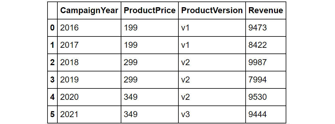
Figure 1.30: Contents of the merged DataFrame

As you can see from the output in Figure 1.30, the DataFrames are merged on the common column (which is CampaignYear). One thing you'll notice is that the data for CampaignYear 2015 is missing. To make sense of this phenomenon, let's understand what is happening behind the scenes.

When we ran the merge() command, pandas merged df_products and df_revenue based on a common column in the two datasets – this was CampaignYear. If there were multiple shared columns in the two datasets, we'd have to specify the exact column we want to merge on as follows:

df_combined = pd.merge(df_products, df_revenue,

                       on = "CampaignYear")

Now, since the CampaignYear column is the only column shared between the two DataFrames and the entry for 2015 is missing in one of the DataFrames (and hence not a shared value), it is excluded in the combined dataset.

What if we still wanted to examine the price and version of the product for 2015 and have revenue as blank for that year? We can fine-tune the merging of DataFrames by using the how parameter.

With the help of the how parameter, you can merge DataFrames in four different  ways:

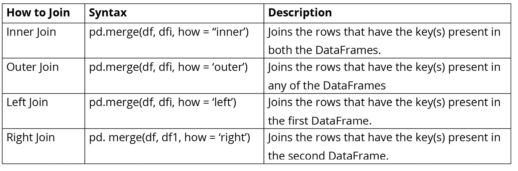
Figure 1.31: Table describing different joins

The following diagram shows two sample DataFrames, df1 and df2, and the results of the various joins performed on these DataFrames:

Figure 1.32: Table showing two DataFrames and the outcomes of different joins on them

In the preceding diagram, outer join returns all the records in df1 and df2 irrespective of a match (any missing values are filled with NaN entries). For example, if we wanted to do an outer join with the products and revenue DataFrames, we would have to run the following command:

df_combined_outer = pd.merge(df_products, df_revenue,

                             how = 'outer')

The output should be as follows:

Figure 1.33: Outer join

You can see that with outer join, even the row that did not match (2015) is included.

Inner join returns records with matching values in df1 and df2. From Figure 1.32, you can see that those are 6 and 7. If you merged the products and revenue DataFrames using an inner join, you'd have the same output that you see in Figure 1.33. By default, pandas uses an inner join.

Left join returns all the records in the left DataFrame and the matched records in the right DataFrame. If any values are missing, it will fill those entries with NaN values. In the products and revenue DataFrames, a left join on the CampaignYear column would return even the row representing 2015, except that the entry for revenue would be NaN.

Right join works similar to left join, except that it returns all the records from the right DataFrame along with just the matching records from the left DataFrame.

So far, you have seen how to merge DataFrames with the same column names. But what if you tried to merge DataFrames containing common data but with differently named columns? In such cases, you will have to specify the column names of the left and the right DataFrame as follows:

df_combined_specific = pd.merge(df_products, df_revenue,

                               left_on="CampaignYear",

                               right_on="CampaignYear2")

In the preceding code block, left_on specifies the column name of the left DataFrame (df_products), while right_on specifies the column name of the right DataFrame (df_revenue).

You have seen how to join DataFrames in this section. In the next section, you will be looking at how to handle missing values.

Handling Missing Data

As a marketing analyst, you will encounter data with missing values quite a lot. For example, let's say you join a Product category table with an Ad viewership table. Upon merging these two, you may find that not all product categories will have a corresponding value in the Ad Viewership table. For example, if a company ran no ads for winter clothes in tropical countries, values for those products in the Ad Viewership table would be missing. Such instances are quite common when dealing with real-world data.

Here's another example of missing data where the category column in the DataFrame has a missing value (demarcated by NaN):

Figure 1.34: Sample DataFrame

While the way you can treat missing values varies based on the position of the missing values and the particular business use case, here are some general strategies that you can employ:

• You can get rid of missing values completely using df.dropna, as explained in the Adding and Removing Attributes and Observations section previously.
• You can also replace all the missing values simultaneously using df.fillna().

When using fillna(), the value you want to fill in will depend heavily on the context and the use case for the data. For example, you can replace all missing values with the mean of the column where the missing value is present:

df.fillna(df.mean())

You should then get the following output:

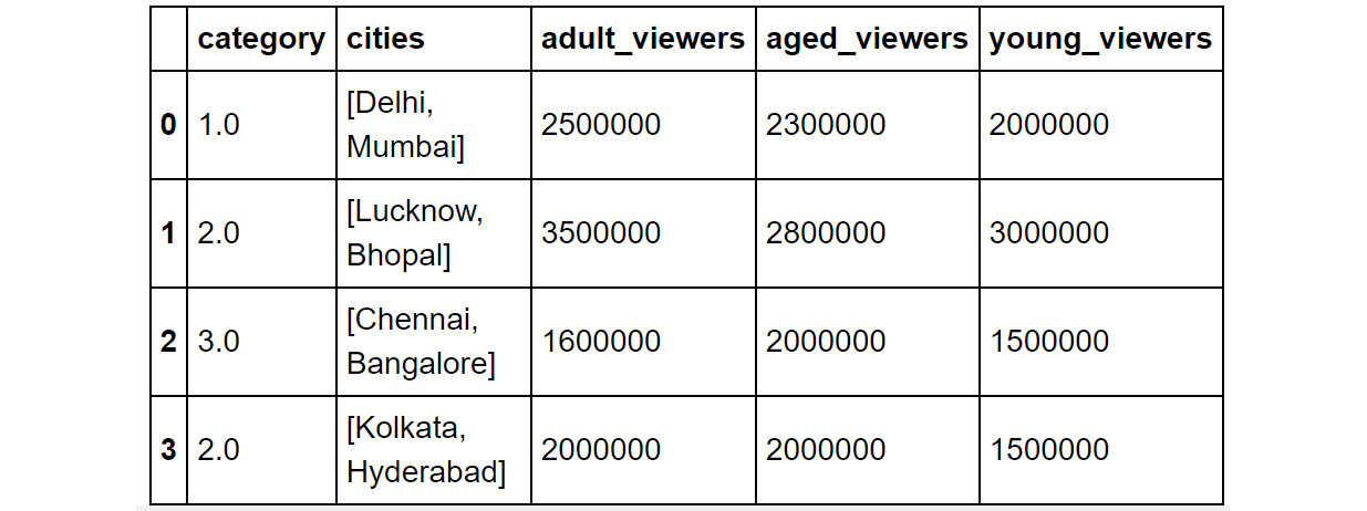
Figure 1.35: Output of the df.fillna(df.mean()) command

Or the median of the data, as in this example:

df.fillna(df.median())

You should then get the following output:

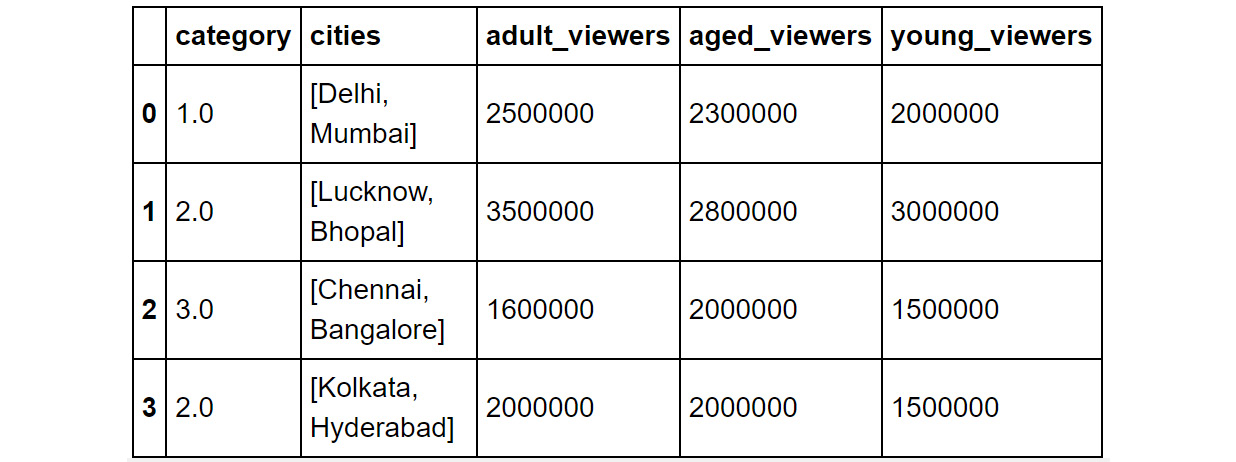
Figure 1.36: Output of the df.fillna(df.median()) command

Or, with some values, such as –1 (or any number of your choice) if you want the record to stand apart during your analysis:

df.fillna(-1)

You should then get the following output:

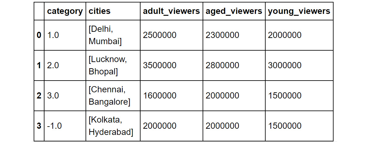
Figure 1.37: Using the df.fillna function

To help deal with missing values better, there are some other built-in functions you can use. These will help you quickly check whether your DataFrame contains any missing values.

You can check for slices containing missing values using the isnull() function:

df.isnull()

This command will return output like the following:

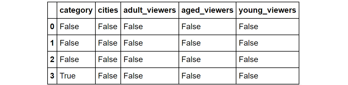
Figure 1.38: Using the .isnull function

The entries where there are null values will show up as True. If not, they'll show up as False.

Similarly, you can check whether individual elements are NA using the isna function. Here, we are using the isna function with the category column:

df[['category']].isna

The command will provide you with a Boolean output. True means that the element is null, and False means it is not:

Figure 1.39: Using the isna function used on a column

In the next exercise, you will be combing different DataFrames and taking care of the missing values.

Exercise 1.03: Combining DataFrames and Handling Missing Values

As part of its forthcoming holiday campaign, the business wanted to understand the cost of acquisition of customers for an e-commerce website specializing in kids' toys. As a marketing analyst, you now have to dig through the historical records of the previous campaign and suggest the marketing budget for the current campaign.

In this exercise, you will be importing two CSV files, timeSpent.csv and cost.csv, into the DataFrames df1 and df2. The df1 DataFrame has the details of the users, along with the time spent on the website. The df2 DataFrame consists of the cost of acquisition of a user.

You will combine the DataFrame containing the time spent by the users with the other DataFrame containing the cost of acquisition of the user. You will merge both these DataFrames to get an idea of user behavior.

Perform the following steps to achieve the aim of this exercise:

1. Import the pandas modules that you will be using in this exercise:

   import pandas as pd

2. Load the CSV files into the DataFrames df1 and df2:

   df1 =pd.read_csv("timeSpent.csv")

   df2 =pd.read_csv("cost.csv")

   Note

   You can find the timeSpent.csv file at https://packt.link/bpfVk and the cost.csv file at https://packt.link/pmpkK.

   Also, do make sure that you modify the path (emboldened) based on where these files are saved on your system.

3. Examine the first few rows of the first DataFrame using the head() function:

   df1.head()

   You should get the following output:

   

   Figure 1.40: Contents of df1

   You can see that the DataFrame, df1, has two columns – users and timeSpent.

4. Next, look at the first few rows of the second dataset:

   df2.head()

   You should get the following output:

   

   Figure 1.41: Contents of df2

   As you can see, DataFrame df2 has two columns – users and cost. In the cost column, there is a NaN value.

5. Do a left join of df1 with df2 and store the output in a DataFrame, df. Use a left join as we are only interested in users who are spending time on the website. Specify the joining key as "users":

   df = df1.merge(df2, on="users", how="left")

   df.head()

   Your output should now look as follows:

   

   Figure 1.42: Using the merge and fillna functions

6. You'll observe some missing values (NaN) in the preceding output. These types of scenarios are very common as you may fail to capture some details pertaining to the users. This can be attributed to the fact that some users visited the website organically and hence, the cost of acquisition is zero.

   These missing values can be replaced with the value 0. Use the following code:

   df=df.fillna(0)

   df.head()

   Your output should now look as follows:

   

Figure 1.43: Imputing missing values with the fillna function

Now, the DataFrame has no missing values and you can compute the average cost of acquisition along with the average time spent. To compute the average value, you will be using the built-in function describe, which gives the statistics of the numerical columns in the DataFrame. Run the following command:

df.describe()

You should then get the following result:

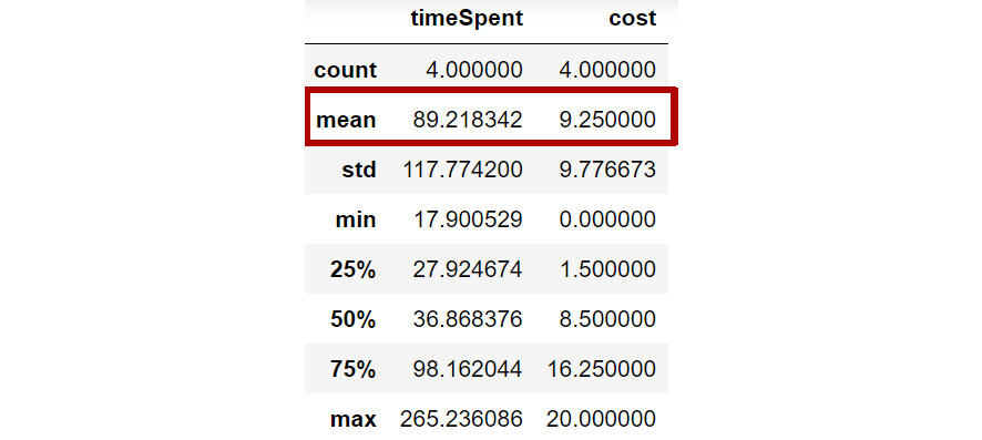
Figure 1.44: Mean value of the columns

From the preceding screenshot, you can infer that the average cost of acquisition of a user is $9.25 and, on average, a user spends around 89 seconds on the website. Based on the traffic you want to attract for the forthcoming holiday season, you can now compute the marketing budget using the following formula:

Marketing Budget = Number of users * Cost of Acquisition

In this exercise, you have successfully dealt with missing values in your data. Do keep in mind that handling missing values is more of an art than science and each scenario might be different. In the next section, you will learn how to apply functions and operations on a DataFrame.

Applying Functions and Operations on DataFrames

By default, operations on all pandas objects are element-wise and return the same type of pandas objects. For instance, look at the following code:

df['viewers'] = df['adult_viewers']

                +df['aged_viewers']+df['young_viewers']

The preceding code will add a viewers column to the DataFrame, with the value for each observation equaling the sum of the values in the adult_viewers, aged_viewers, and young_viewers columns.

Similarly, the following code will multiply every numerical value in the viewers column of the DataFrame by 0.03 or whatever value you want to keep as your target CTR (click-through rate):

df['expected clicks'] = 0.03*df['viewers']

Hence, your DataFrame will look as follows once these operations have been performed:

Figure 1.45: Operations on pandas DataFrames

pandas also supports several built-in functions on pandas objects:

Figure 1.46: Built-in functions used in pandas

Note

Remember that pandas objects are Python objects, too. Therefore, you can write your custom functions to perform specific tasks on them.

To apply built-in or custom functions to pandas, you can make use of the map and apply functions. You can pass any built-in, NumPy, or custom functions as parameters to these functions and they will be applied to all elements in the column:

• map: map executes a function on each value present in the column. For example, look at the following DataFrame:

Figure 1.47: A sample DataFrame

Now, suppose you want to change the values of the Gender column to denote Female as F and Male as M. This can be achieved with the help of the map function. You'll need to pass values to the map function in the form of a dictionary:

df['Gender']=df['Gender'].map({"Female":"F","Male":"M"})

You should get the following result:

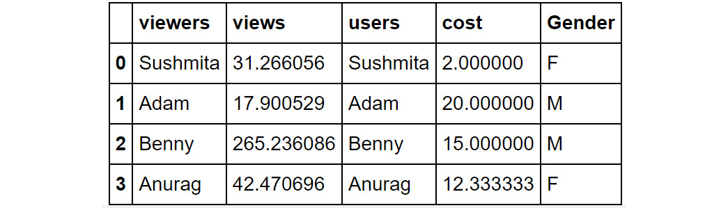
Figure 1.48: Using the map function

In the preceding screenshot, you can see that the values in the Gender column are now displayed as M and F.

• apply: This applies the function to the object passed and returns a DataFrame. It can easily take multiple columns as input. It also accepts the axis parameter, depending on how the function is to be applied. For example, let's say in the following DataFrame you wanted to sum all the purchases made by the user across the different categories and store the sum in a new column:

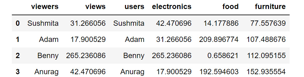
Figure 1.49: Sample DataFrame

You can achieve this with the help of the apply function as follows:

df1['purchase']=df1[['electronics','food','furniture']]

                .apply(np.sum,axis=1)

df1

Note

In the preceding code, since you're using NumPy, you will need to import the numpy library before trying out the code. You can do so by using import numpy as np.

You should then get the following result:

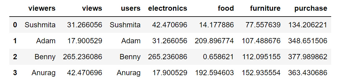
Figure 1.50: Using the apply function

In the preceding screenshot, you can see that a new column, purchase, is created, which is the sum of the electronics, food, and furniture columns.

In this section, you have learned how to apply functions and operations to columns and rows of a DataFrame. In the next section, you will look at how to group data.

Grouping Data

Let's suppose, based on certain conditions, that you wanted to apply a function to multiple rows of a DataFrame. For example, you may need to do so when you want to calculate the sum of product prices separately for each currency. The pythonic way to solve this problem is to slice the DataFrame on the key(s) you want to aggregate on and then apply your function to that group, store the values, and move on to the next group. pandas provides a better way to do this, using the groupby function.

Let's look at the following DataFrame:

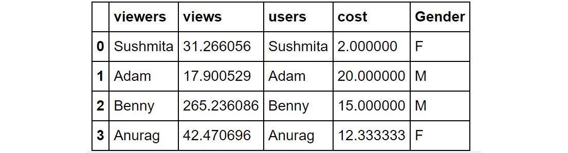
Figure 1.51: Sample DataFrame

If you want to find out the total cost of acquisition based on gender, you can use the following code:

df.groupby('Gender')['cost'].sum()

You should then get the following output:

Figure 1.52: Using the groupby function

In the preceding screenshot, you can see that the male users have a higher cost of acquisition than female users. In the next exercise, you will implement some of the operations you have learned so far.

Exercise 1.04: Applying Data Transformations

In Exercise 1.01, Loading Data Stored in a JSON File, you worked with a JSON file that contained the details of the users of a shopping app. There, your task was to validate whether the data was loaded correctly and to provide some answers about the information contained in it. Since you confirmed that the data was loading correctly, you'll be working with the same dataset once again, but this time, you'll be analyzing the underlying data. Also, this time, you'll be answering some interesting questions that the marketing team has come up with:

• What is the average age of the users?
• Which is the favorite fruit of the users?
• Do you have more female customers?
• How many of the users are active?

This exercise aims to get you used to performing regular and groupby operations on DataFrames and applying functions to them. You will use the user_info.json file on GitHub.

Note

You can find the user_info.json file at the following link: https://packt.link/Gi2O7.

1. Import the pandas module using the following command:

   import pandas as pd

2. Read the user_info.json file into a pandas DataFrame, user_info, using the following command:

   user_info = pd.read_json('user_info.json')

   Note

   Make sure you change the path (emboldened) to the JSON file based on its location on your system. If you're running the Jupyter notebook from the same directory where the JSON file is stored, you can run the preceding code without any modification.

3. Now, examine whether your data is properly loaded by checking the first few values in the DataFrame. Do this using the head() command:

   user_info.head()

   You should get the following output:

   

   Figure 1.53: Output of the head function on user_info

   Note

   Not all columns and rows are shown in the preceding output.

   The data consists of session information of the customers, along with their demographic details, contact information, and other details.

4. Now, look at the attributes and the data inside them using the following command:

   user_info.info()

   You should get the following output:

   

   Figure 1.54: Output of the info function on user_info

5. Now, let's start answering the questions:

   What is the average age of the users? To find the average age, use the following code:

   user_info['age'].mean()

   You will get the output as 27.83, which means that the average age of the users is 27.83.

   Which is the favorite fruit among the users? To answer this question, you can use the groupby function on the favoriteFruit column and get a count of users with the following code:

   user_info.groupby('favoriteFruit')['_id'].count()

   You should get the following output:

   

Figure 1.55: Output of the count function

From the preceding screenshot, you can see that there is no clear winner as both apple and strawberry have the same count of 3.

Do you have more female customers? To answer this question, you need to count the number of male and female users. You can find this count with the help of the groupby function. Use the following code:

user_info.groupby('gender')['_id'].count()

You should get the following output:

Figure 1.56: Output of the count function

From the preceding screenshot, you can infer that you have an equal split of customers concerning gender. Now, let's move on to our last question.

How many of the users are active? Similar to the preceding questions, you can use the groupby function on the isActive column to find out the answer.

Use the following code:

user_info.groupby('isActive')['_id'].count()

You should get the following output:

Figure 1.57: Output of the count function

From the preceding screenshot, you see that three customers are active while the other three are inactive.

This exercise acts as a short introduction to applying data transformations, functions, and getting an overview of aggregation, which can come in handy during the exploratory phase of a project.

Now that you have learned the different aspects of data preparation and cleaning, let's test your skills with the help of the following activity.

Activity 1.01: Addressing Data Spilling

The data we receive in most cases is not clean. There will be issues such as missing values, incorrect data types, data not loaded properly in the columns, and more. As a marketing analyst, you will have to clean this data and render it in a usable format so that you can analyze it further to mine useful information.

In this activity, you will now solve the problem that you encountered in Exercise 1.02, Loading Data from Multiple Sources. You will start by loading sales.csv, which contains some historical sales data about different customer purchases in stores in the past few years. As you may recall, the data loaded in the DataFrame was not correct as the values of some columns were getting populated wrongly in other columns. The goal of this activity is to clean the DataFrame and make it into a usable form.

You need to read the files into pandas DataFrames and prepare the output so that it can be used for further analysis. Follow the steps given here:

1. Open a new Jupyter notebook and import the pandas module.
2. Load the data from sales.csv into a separate DataFrame, named sales, and look at the first few rows of the generated DataFrame.

   Note

   You can find the sales.csv file at https://packt.link/IDGB4.

   You should get the following output:

   

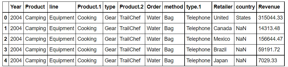
   Figure 1.58: Output of the head function on sales.csv

3. Analyze the data type of the fields.
4. Look at the first column. If the value in the column matches the expected values, move on to the next column or otherwise fix it with the correct value.
5. Once you have fixed the first column, examine the other columns one by one and try to ascertain whether the values are right.

   Hint

   As per the information from the product team, the file contains information about their product line, which is camping equipment, along with information about their flagship product.

   Once you have cleaned the DataFrame, your final output should appear as follows:

   

Figure 1.59: First few rows of the structured DataFrame

Note

The solution to this activity can be found via this link.

Summary

In this chapter, you have learned how to structure datasets by arranging them in a tabular format. Then, you learned how to combine data from multiple sources. You also learned how to get rid of duplicates and needless columns. Along with that, you discovered how to effectively address missing values in your data. By learning how to perform these steps, you now have the skills to make your data ready for further analysis.

Data processing and wrangling are the most important steps in marketing analytics. Around 60% of the efforts in any project are spent on data processing and exploration. Data processing when done right can unravel a lot of value and insights. As a marketing analyst, you will be working with a wide variety of data sources, and so the skills you have acquired in this chapter will help you to perform common data cleaning and wrangling tasks on data obtained in a variety of formats.

In the next chapter, you will enhance your understanding of pandas and learn about reshaping and analyzing DataFrames to visualize and summarize data better. You will also see how to directly solve generic business-critical problems efficiently.