
Chapter 2
Understanding Data
We work with data every day in our business and personal lives. But how often do we stop and think about how our data is structured? Effective data analysts understand data in all its forms and how that data fits into their working environment. Knowledge of data includes understanding the various types of data that exist and the different options for storing that data in an enterprise environment. With a basic grounding in how to think about data, you will be well positioned to meaningfully contribute to the collection, organization, and analysis of data.
We will kick off this chapter by examining data types that categorize individual pieces of data and exploring considerations for dealing with the range of possible values for different data types. We will learn how these building blocks are combined to describe a unique object or event in the sections that follow. We will also explore different ways of organizing data and various file formats for facilitating data exchange, system interoperability, and ease of human consumption.
Exploring Data Types
To understand data types, it is best first to understand data elements. A data element is an attribute about a person, place, or thing containing data within a range of values. Data elements also describe characteristics of activities, including orders, transactions, and events. Consider the data in Table 2.1, which illustrates some simple information about domesticated animals. We can see that the data elements include the name, type, breed, date of birth, height, and weight for each animal in the table. The column headings name the data element, while each row is an example value for that element.
TABLE 2.1 Pet data
| Pet Name | Animal Type | Breed Name | Date of Birth | Height (inches) | Weight (pounds) |
|---|---|---|---|---|---|
| Jack | Dog | Corgi | 3/2/2018 | 10 | 26.3 |
| Viking | Dog | Husky | 5/8/2017 | 24 | 58 |
| Hazel | Dog | Labradoodle | 7/3/2016 | 23 | 61 |
| Schooner | Dog | Labrador Retriever | 8/14/2019 | 24.3 | 73.4 |
| Skippy | Dog | Weimaraner | 10/3/2018 | 26.3 | 63.5 |
| Alexander | Cat | American Shorthair | 10/4/2017 | 9.3 | 10.4 |
Now that you understand what data elements are, let's explore how they relate to data types. A data type limits the values a data element can have. Consider the information in Table 2.1. Pet Name, Animal Type, and Breed Name are all words. Meanwhile, the Date of Birth column contains numbers and slashes that identify a specific date. Height and Weight are both numbers. Each of these groupings represents a particular data type.
Individual data types support structured, unstructured, and semi-structured data. Let's explore the differences between these categories.
Structured Data Types
Structured data is tabular in nature, organized into rows and columns. Structured data is what typically comes to mind when looking at a spreadsheet. With clearly defined column headings, spreadsheets are easy to work with and understand. In a spreadsheet, cells are where columns and rows intersect.
Consider the dataset in Figure 2.1. It contains basic information about a group of people. When you read the column headings, you get a good sense of the kind of data that you're going to find in that column. For example, when you see the “Weight (pounds)” column, you expect to see numeric values. In the Address field, you expect to see text. Looking more closely, we see that the data values are consistent for each column. For example, all the height and weight information uses numbers instead of words. Taken as a whole, Figure 2.1 is an example of highly structured data, with defined columns, an expectation for what the rows will contain, and consistent columnar values in each row.

FIGURE 2.1 Person Data
Let's explore some of the most common data types that give structured data its structure.
Character
The character data type limits data entry to only valid characters. Characters can include the alphabet that you might see on your keyboard, as well as numbers. Depending on your needs, multiple data types are available that can enforce character limits.
Alphanumeric is the most widely used data type for storing character-based data. As the name implies, alphanumeric is appropriate when a data element consists of both numbers and letters. Consider the Address field in Figure 2.1. To accurately represent a given street address, both the house number and the street name are required.
The alphanumeric data type is ideal for storing product stock-keeping units (SKUs). It is common in the retail clothing space to have a unique SKU for each item available for sale. If you sell jeans, you may stock products from Armani Jeans, Diesel, Lee Jeans, Levi's, and Wrangler. To keep track of all the manufacturer, size, color, and fit combinations in your inventory, you might use an SKU similar to the one depicted in Figure 2.2. Tracking inventory at the SKU level allows you to manage availability in your online and in-store systems, all courtesy of the alphanumeric data type.
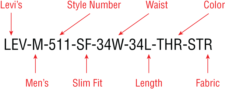
FIGURE 2.2 SKU example
There are times when it is necessary to impose even stricter limits on character-related data to exclude numbers. Excluding numbers can be achieved using the text data type. Closely related to the alphanumeric data type, it is even more stringent. It is helpful to think of text as a subset of alphanumeric, only allowing the storage of alphabetic characters. One practical use of the text data type is to improve the overall data quality. For example, consider the “State” data element in Figure 2.1. If the system contains state names from the United States, it would be appropriate to select a text data type.
Consider a data entry example. Suppose you operate an online retail system. To deliver orders, you need address information for the intended recipients. This information comes from the customers themselves, since they can specify where orders should be shipped. Any time a person interacts with a computer, there is the potential for a data entry error. Suppose someone wanted to enter “Montana” for the state component of their address.
Take a look at the positioning of the O and 0 keys in Figure 2.3, depicting the U.S. QWERTY keyboard layout. These two keys are very close together. Many people press these keys with the fourth finger of their right hand, making a data entry error that much more likely. A person could supply the value “M0ntana” instead of the intended “Montana.” With “State” as a text data type, trying to input the erroneous value would result in an error. However, with “State” implemented as alphanumeric, nothing would prevent that mistake from making its way into the database.

FIGURE 2.3 U.S. QWERTY keyboard layout
Each database software has its unique method of implementing character data types to handle the nuances related to character data. The most significant difference has to do with how much data a particular data element can contain. Table 2.2 shows a sampling of how the three most popular databases provide data types for character data.
All of the data types shown in Table 2.2 support alphanumeric data. Where they differ is on how much data they can handle. Before defining a column as alphanumeric, you need to determine how long your longest-possible text value will be. You also need to realize that while data types may have the same names, they are implemented differently by software vendors. There are also individual data types, like CLOB and LONGTEXT, that are vendor-specific. Finally, you need to be aware of the absolute limits imposed by the database you are using.
TABLE 2.2 Selected character data types and maximum size
| Data type name | Oracle | Microsoft SQL Server | MySQL |
|---|---|---|---|
| char | 2,000 bytes | 8,000 bytes | 255 bytes |
| varchar2 | 4,000 bytes | - | - |
| varchar | - | 8,000 bytes | 64 KB |
| CLOB | 128 TB | - | - |
| varchar(max) | - | 2 GB | - |
| LONGTEXT | - | - | 4 GB |
With spreadsheets, configuring a given cell or range of cells as a text-only data type takes more effort than when using a database. It is not possible to accomplish this with one of the native data types provided by the software. Instead, limiting to just text requires a formula. Figure 2.4 shows an example of how to use a formula to perform this level of validation in Microsoft Excel. Suppose a person tries to input a value containing numbers or symbols into a cell where the formula is active. Figure 2.5 illustrates the resulting error message.

FIGURE 2.4 Excel text-only formula
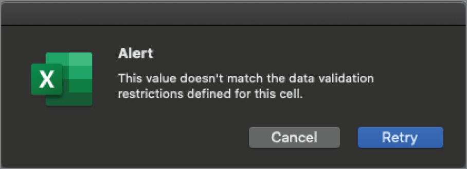
FIGURE 2.5 Text-only data validation restriction
Numeric
When numbers exclusively make up values for a data attribute, numeric becomes the data type of choice. This data type appears to be simple and obvious based on its name. As seen with the character data type, implementation nuances about numeric are essential to understand. Databases accommodate two types of numeric data types: integer and numeric.
Whole Numbers
The integer, and all its subtypes, are for storing whole numbers. As seen with the character family of data types, implementation differences exist across databases. Table 2.3 illustrates how Oracle, Microsoft, and MySQL support whole numbers.
Note that both the Microsoft and MySQL databases support the bit data type, which can be empty or store a 0 or a 1. In computer science, flags indicate whether something is on or off, or if a function has completed successfully. To show something is on, 1 or TRUE is used. For a value of off, 0 or FALSE is used. The bit data type is intended for storing the status of a flag.
Note also that the value ranges for smallint and shortinteger are identical. The same is true for int and integer, as well as bigint and longinteger. Although the data types have different names, their functionality is equivalent.
Rational Numbers
In all its variants, the numeric data type is for rational numbers that include a decimal point. As with the integer family of data types, each database vendor has its implementation nuances. Table 2.4 illustrates how Oracle, Microsoft, and MySQL support rational numbers.
TABLE 2.3 Selected integer data types and value range
| Data type name | Oracle | Microsoft SQL Server | MySQL |
|---|---|---|---|
| bit | - | 0 and 1 | 0 and 1 |
| tinyint | - | 0 to 255 | 0 to 255 |
| smallint | - | –32,768 to 32,767 | –32,768 to 32,767 |
| shortinteger | –32,768 to 32,767 | - | - |
| int | - | –2,147,483,648 to 2,147,483,647 | –2,147,483,648 to 2,147,483,647 |
| integer | –2,147,483,648 to 2,147,483,647 | - | - |
| bigint | - | –9,223,372,036,854,775,808 to 9,223,372,036,854,775,807 | –9,223,372,036,854,775,808 to 9,223,372,036,854,775,807 |
| longinteger | –9,223,372,036,854,775,808 to 9,223,372,036,854,775,807 | - | - |
TABLE 2.4 Selected integer data types and value range
| Data type name | Oracle | Microsoft SQL Server | MySQL |
|---|---|---|---|
| shortdecimal | –10^38 to 10^38, up to 7 significant digits | - | - |
| number | –10^125 to 10^125, up to 38 significant digits | - | - |
| decimal | –10^308 to 10^308, up to 15 significant digits | –10^38 to 10^38, up to 38 significant digits | Up to 65 digits in total, so the range depends on the number of digits assigned to the whole and fractional components |
You must take several factors into account when dealing with rational numbers. In both SQL Server and MySQL, there is a data type called numeric that is functionally equivalent to the decimal data type. Realizing that data types are inconsistently named across databases, you need to consider the ultimate range of values a given data element handles. All the data types in Table 2.4 store numbers to a configurable number of significant digits. There are scientific use cases that require an even greater number of significant digits; additional numeric data type variants exist to accommodate that need.
Date and Time
Gathered together under the broad category of date, day of year and time of day are data elements that appear with great frequency. As illustrated in Table 2.5, databases have various data types for handling date- and time-related information. As seen with character and numeric data types, nuances exist across different databases. Selecting the appropriate date-related data type depends on the data you need to store.
TABLE 2.5 Selected date and time data types
| Data type name | Oracle | Microsoft SQL Server | MySQL |
|---|---|---|---|
| date | YYYY-MM-DD | YYYY-MM-DD | YYYY-MM-DD |
| datetime2 | - | YYYY-MM-DD hh:mm:ss.sss[.fractional seconds] | YYYY-MM-DD hh:mm:ss.sss[.fractional seconds] |
| time | - | hh:mm:ss.sss[.fractional seconds] | YYYY-MM-DD hh:mm:ss.sss[.fractional seconds] |
| timestamp | YYYY-MM-DD hh:mm:ss.sss[.fractional seconds] | - | - |
| year | - | - | YYYY |
For example, suppose you operate a veterinary clinic and need to store birth date information for pets. In that case, you need to store the year, month, and day. With those three components of date, you can effectively administer medication and determine when to schedule annual veterinary appointments.
There are many occasions when it is more appropriate to include time, in addition to the day, month, and year. For instance, consider package tracking information for companies like FedEx, United Parcel Service, or DHL. Consumers want to know where a specific package is up to the minute. The company itself may need second-level details to optimize labor, infrastructure investments, and route planning.
Currency
Many people use spreadsheets to manage their finances. Organizations typically use enterprise-scale software for the same purpose, with the data residing in a database. While financial data is numeric, people prefer seeing the numbers displayed as a specific currency. For example, consider the Number, Dollar, and Euro columns in Figure 2.6. The column headings indicate what each column contains. The currency symbols in each cell tell the reader what the data represents, even if the column headings have scrolled off the screen.
Especially in this context, it is essential to differentiate between data formatting and data storage. Data storage contains the actual value for a given data element. Data formatting takes a given data value and then formats it for display purposes. Data formatting is common when dealing with currency and date data types.
The numeric data in all the columns of Figure 2.6 are numerically equivalent. Figure 2.7 illustrates a sampling of currencies available for formatting in a Google spreadsheet.
Of the databases mentioned in this chapter, only Microsoft SQL Server has data types specifically for storing currency. Table 2.6 illustrates these two data types. Both of these data types offer four digits of precision after the decimal point.
TABLE 2.6 Currency data types in Microsoft SQL Server
| Data type name | Range of values |
|---|---|
| smallmoney | –214,748.3648 to 214,748.3647 |
| money | –922,337,203,685,477.5808 to 922,337,203,685,477.5807 |
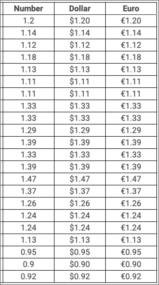
FIGURE 2.6 Numeric data formatted as different currencies

FIGURE 2.7 Currency formats in Google Sheets
While the currency data types exist, it is more common to use a numeric data type for storing currency data. Limiting a calculation to only four digits of precision after the decimal point can lead to incorrect rounding errors. Consider Figure 2.8, which illustrates retrieving values from a database. The money_table_example table contains columns defined as money for both sales price and price. The percentage column in the query result is calculated by taking the sales price divided by the price and then multiplying the result by 100. Figure 2.9 illustrates the same calculation in a spreadsheet, and Figure 2.10 shows the result of 18 divided by 22 in a calculator.
Recall that the money data type uses only four digits after the decimal. For this reason, the database incorrectly calculates the percentage as 81.81 instead of the spreadsheet's correct evaluation of 81.82.
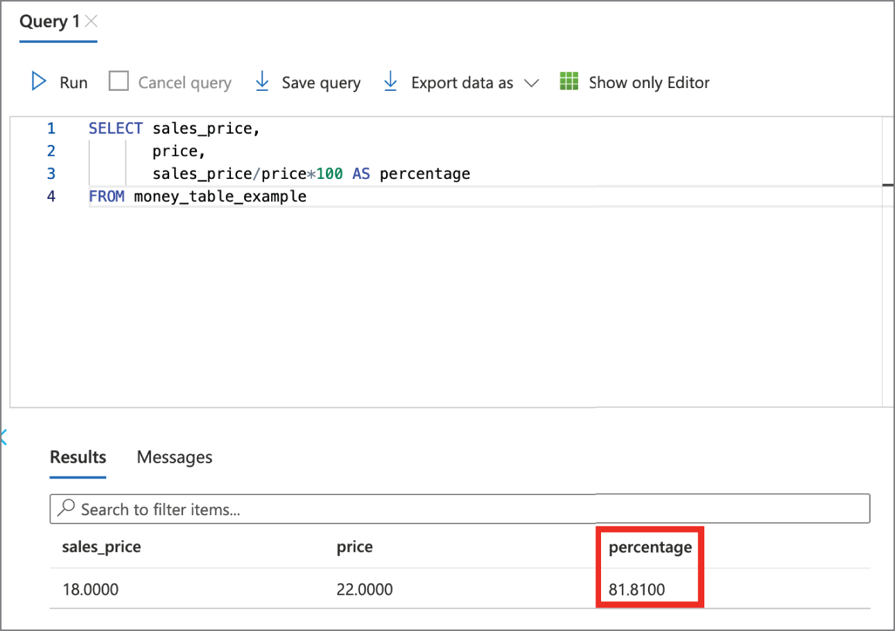
FIGURE 2.8 Incorrect percentage due to money data type

FIGURE 2.9 Correct percentage as calculated by a spreadsheet
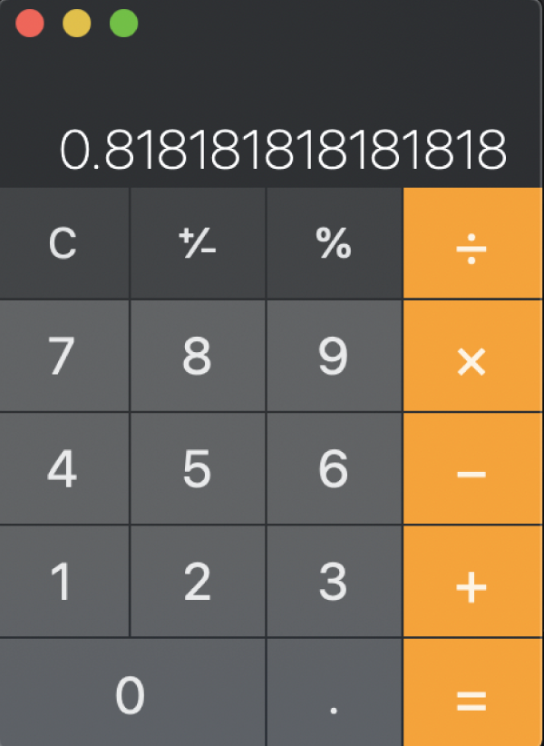
FIGURE 2.10 Unrounded calculation in a calculator
While SQL Server does support two currency-specific data type variants, most databases do not. As the rounding error in Figure 2.8 shows, it is best to use a numeric data type to store currency-related data. Figure 2.11 illustrates that the rounded results are mathematically accurate using the numeric data type for both sales_price and price.

FIGURE 2.11 Correct percentage when using a numeric data type
Unstructured Data Types
While much of the data we use to record transactions is highly structured, most of the world's data is unstructured. Unstructured data is any type of data that does not fit neatly into the tabular model. Examples of unstructured data include digital images, audio recordings, video recordings, and open-ended survey responses. Analyzing unstructured data creates a wealth of information and insight. Many people have camera-enabled smartphones, and using video for conversations and meetings is commonplace. To capture and analyze unstructured data, we make use of data types designed explicitly for that purpose.
Consider the pet data depicted in Table 2.1. Suppose the veterinary office wants to augment their records to include digital images of the animals. To accommodate that requirement, we need to make use of an unstructured data type.
Binary
Binary data types are one of the most common data types for storing unstructured data. It supports any type of digital file you may have, from Microsoft Excel spreadsheets to digital photographs. When considering which binary data type to use, file size tends to be the limiting factor. You need to select a data type that is as large as the largest file you plan on storing.
The most common types of unstructured data are audio, image, and video data. Spreadsheets are consumer applications designed to manage highly structured data, but they're often not very good at storing binary data. Figure 2.12 illustrates the result of trying to integrate images into the pet information spreadsheet in Excel. While it is possible to place images within the spreadsheet, it is impossible to store the images within a cell. However, Google Sheets does allow the storing of binary data within a cell, as shown in Figure 2.13.

FIGURE 2.12 Images in Excel
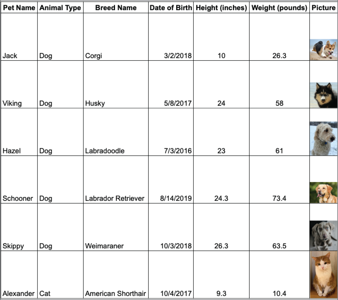
FIGURE 2.13 Binary data in a Google spreadsheet
Databases offer a much more sophisticated collection of data types for storing binary data, as Table 2.7 illustrates. Note that the maximum size is per row, not per table. Once again, we see the inconsistency in naming, as well as supported size.
TABLE 2.7 Selected binary data types and maximum sizes
| Data type name | Oracle | Microsoft SQL Server | MySQL |
|---|---|---|---|
| tinyblob | - | - | 255 bytes |
| mediumblob | - | - | 16 MB |
| binary | - | 8,000 bytes | 64 MB |
| varbinary | - | - | 64 MB |
| varbinary(max) | - | 2 GB | - |
| longblob | - | - | 4 GB |
| BLOB | 128 TB | - | 64 KB |
Audio
Audio data can come from a variety of sources. Whenever you interact with a customer service agent and hear “this call may be recorded for quality assurance purposes,” your conversation is probably being recorded and stored for later analysis. The impact of capturing, storing, and analyzing audio data has led to the development of avalanche detection systems. These systems listen for and detect the acoustic characteristics of an avalanche. With real-time notification capabilities, these systems reduce the time it takes for emergency services to respond and alert hikers to treacherous conditions.
In order to ingest audio data into a system and make it available for processing, data is first captured via a microphone. The data is then digitized and stored. Audio can be stored in its raw form, which consumes the most storage space. Alternatively, it can be encoded with a compression algorithm to reduce the amount of space required. Regardless of if it is in raw or compressed form, storing audio requires a data type designed to handle raw binary data.
Images
Image data can come from a variety of sources. People take more than 1 trillion photographs every calendar year, fueled by the ubiquity of camera-enabled smartphones and relatively low storage costs. Each digital picture is a piece of unstructured data. Examining Figure 2.14, it is easy for a human to identify the contents of the photograph. However, it is a binary file to a computer, ultimately stored as a series of ones and zeros. Applying artificial intelligence algorithms for image processing over a set of digital photos allows people to look for the objects they contain. Figure 2.15 illustrates the search results for the word “motorcycle” in a digital image library.

FIGURE 2.14 Photograph of racing motorcycles

FIGURE 2.15 Motorcycle search results
Image data has applicability across several industries. For example, dentists use digital X-rays to augment a person's dental record. Magnetic resonance imaging scans, used for soft tissue investigations, are added to a person's health record. Insurance companies provide mobile applications to upload photographs of accident scenes. As the use of image data grows, understanding how it is stored is vital for the modern data analyst.
Resolution is the most significant factor that governs how much space is required to store an image. The greater the resolution, the more detail an image contains, and the more storage space it needs. Similar to compressing audio data, there are a variety of ways to encode and store images. Storing images in a database requires a data type designed to handle raw binary data, such as varbinary or BLOB.
Video
Video data is growing at a similar pace to image data. In the consumer space, people upload videos to YouTube, Instagram, and TikTok every day. Police officers wear body cameras to create a video record of enforcement situations. Image processing algorithms examine videos to detect everything from traffic congestion to intruders in the home.
As is the case with audio data, the resolution has a significant impact on the storage a video consumes. Video duration is also another factor that impacts storage size. Consider Table 2.8, which approximates the space required for storing a still image, one minute of audio data, and one minute of video data as recorded on a modern smartphone. We see that every minute of video is equivalent to over 50 individual images, or more than 200 minutes of audio.
TABLE 2.8 Approximate storage needs
| Still image | Audio (1 minute) | Video (1 minute) | |
|---|---|---|---|
| Space consumed (KB) | 2,048 | 503 | 102,400 |
Large Text
There are times when it is appropriate to store a significant amount of text data. It is the combination of words into sentences that result in classifying large text as unstructured data. You may need to explore text data to detect nuance, humor, sarcasm, and inferential meaning. For example, you may need to keep the complete transcript of a legal proceeding, public address, or verbose open-ended survey responses. What differentiates large text from the text and alphanumeric data types is size. When considering Table 2.9, keep in mind that 2 GB of character data is approximately 1 million pages of text.
TABLE 2.9 Selected binary data types and maximum sizes
| Data type name | Oracle | Microsoft SQL Server | MySQL |
|---|---|---|---|
| varchar(max) | - | 2 GB | - |
| longtext | - | - | 4 GB |
| CLOB | 128 TB | - | - |
Once again, note that data type names differ across vendor products. For example, Table 2.2 shows that Oracle has the varchar2 text data type. Oracle currently implements varchar as a synonym for varchar2. However, Microsoft's implementation of varchar is vastly different. In Oracle, since the varchar data type is a synonym of varchar2, it is limited to 4,000 bytes. Meanwhile, Microsoft's implementation of varchar supports up to 2 GB. To handle larger amounts of text, Oracle created the proprietary CLOB data type.
Categories of Data
We try to fit data into structured and unstructured categories. The reality is that the world is not black and white, and not all data fits neatly into structured and unstructured categories. Semi-structured data represents the space between structured spreadsheets and unstructured videos.
As illustrated in Table 2.1, a veterinary practice may be interested in collecting structured data about the animals under its care. When mapping data attributes to data types, there are additional considerations regarding the actual values to be stored.
Quantitative vs. Qualitative Data
Regardless of structure, data is either quantitative or qualitative. Quantitative data consists of numeric values. Data elements whose values come from counting or measuring are quantitative. In Table 2.1, the Height and Weight columns are quantitative. Quantitative data answers questions like “How many?” and “How much?”
Qualitative data consists of frequently text values. Data elements whose values describe characteristics, traits, and attitudes are all qualitative. In Table 2.1, Pet Name, Animal Type, and Breed Name are all qualitative. Qualitative data answers questions like “Why?” and “What?”
Discrete vs. Continuous Data
Numeric data comes in two different forms: discrete and continuous. A helpful way to think about discrete data is that it represents measurements that can't be subdivided. You may intuitively think of discrete data as using whole numbers, but that doesn't have to be the case. For example, if a fundraising organization sells chickens in half-chicken increments, you can buy 1.5 chickens. However, you can't buy .25 chickens.
Another way to think about it is that discrete data is useful when you have things you want to count. For example, a veterinary clinic may be interested in the number of dogs and cats under its care. Figure 2.16 shows the aggregation of the pet from Table 2.1. The Total data element is an example of discrete data, as it contains the value 5 for Dog and 1 for Cat. A veterinary practice would not care for 5.5 dogs or 2.25 cats.
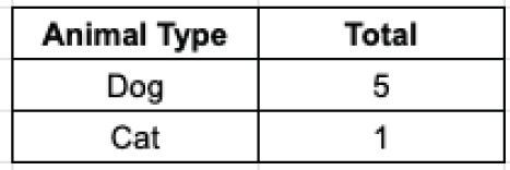
FIGURE 2.16 Discrete data example
Instead of counting, when you measure things like height and weight, you are collecting continuous data. While whole numbers represent discrete data, continuous data typically need a decimal point. Two dogs in Table 2.1 have their height recorded to the tenth of an inch. Similarly, weight is recorded to the tenth of an inch for three dogs and one cat. Figure 2.17 shows the continuous measure of average height and weight information by animal.

FIGURE 2.17 Continuous data example
Both the Average Height and Average Weight calculations for dogs result in numbers to the hundredths. These averages will change as the animals' weight changes and as the veterinarian's practice grows and adds animals. In addition, the degree of precision in terms of weight measurement could change. For example, the vet could start recording weight information to the hundredths instead of the tenths. The Height and Weight attributes from Table 2.1, as well as the Average Height and Average Weight from Figure 2.17, are examples of continuous data elements.
Qualitative data is discrete, but quantitative data can be either discrete or continuous data. For example, age is a continuous variable, but you may treat a person's age in years as discrete. A good rule of thumb is that discrete applies when counting while continuous applies when measuring.
Categorical Data
In addition to quantitative, numeric data, there is categorical data. Text data with a known, finite number of categories is categorical. When considering an individual data element, it is possible to determine whether or not it is categorical. Let's continue to identify each data element of the pet dataset in Table 2.1. Animal Type is a good example of categorical data. As represented, this column separates the data into two categories: dog and cat. As additional dogs or cats enter into care, they fall within the existing categories.
That said, the range of accepted values for a given category can change over time. For instance, suppose the veterinarian branches out beyond small animal care and starts caring for horses. It is possible to expand the range of acceptable values in a category to accommodate this change.
You can also use categories to enforce data validation when someone is first entering data. Category enforcement has the effect of improving data quality. For example, suppose the veterinarian decides to only care for cats and dogs. To streamline operations, the veterinarian has a website built so that clients can schedule appointments online. Suppose the intent is to limit online appointments only for dogs and cats. In that case, the website can implement a drop-down menu where the only options for the animal type are “dog” and “cat.” If someone had a mouse, hamster, or gerbil, the validation check prevents the scheduling of an appointment.
Dimensional Data
Dimensional modeling is an approach to arranging data to facilitate analysis. Dimensional modeling organizes data into fact tables and dimension tables. Fact tables store measurement data that is of interest to a business. A veterinary practice may want to answer some questions about appointments. A table holding appointment data would be called a fact table.
Dimensions are tables that contain data about the fact. For appointment data, the veterinarian's office manager may want to understand who was at an appointment and if any procedures were performed. In Figure 2.18, the Appointments table is the fact table. The Veterinarians, Owners, Procedures, and Pets tables are all dimensions that can answer questions about appointments.

FIGURE 2.18 Dimension illustration
Dimensional data contains groupings of individual attributes about a given subject. For example, taken as a whole, the pets dataset from Table 2.1 can be called the “pets” dimension. You can imagine that the “owners” dimension in Figure 2.18 contains biographic information about a pet's owner, identifying who was present at an appointment. When combined with data from additional dimensions, data elements from each dimension add detail about the facts in the fact table. We will explore dimensional modeling in greater detail in Chapter 3.
Common Data Structures
In order to facilitate analysis, data needs to be stored in a consistent, organized manner. When considering structured data, several concepts and standards inform how to organize data. On the other hand, unstructured data has a wider variety of storage approaches.
Analysts need to be able to perform their roles as efficiently as possible. It is common to use multiple tools to analyze data. Improved integration and interoperability between tools makes it easier for analysts to be productive. As a result, several concepts have become standardized. Let's explore the similarities and differences in how structured and unstructured data is defined and organized.
Structured Data
Tabular data is structured data, with values stored in a consistent, defined manner, organized into columns and rows. Data is consistent when all entries in a column contain the same type of value. This method of organization facilitates aggregation. For example, you can add each value in the Weight column in Table 2.1 to get the total weight for all animals. Structured data also makes summarization easy, since you can compute the average height for each animal in Table 2.1. It is common to perform summarization across groups. Figure 2.17 illustrates summarization at the categorical level.
However, structured data does not translate directly to data quality. For example, suppose a new dog named Thor became a patient. When Thor's data was input into the system, a person transposed the Pet Name and Animal Type values, as highlighted in Figure 2.19. Since both Pet Name and Animal Type are character data types, nothing from a structural standpoint prevents this mistake. However, if you were to perform the same summarization as in Figure 2.16, the result would be what is represented by Figure 2.20. A person looking at the summary in Figure 2.20 would immediately know that something is amiss from a data quality standpoint, as “Thor” is not a type of animal.

FIGURE 2.19 Data entry error

FIGURE 2.20 Data entry error identified in a summary
Just as there is an expectation that the values in a given column are consistent, it is a convention that each row contains data about a single record. In Figure 2.19, each row contains data about a single animal. Once again, nothing structural prevents a person from incorrectly putting data about Thor into Alexander's row. However, the intent is that each row's data pertains to a single animal.
It is a best practice to specify a key that uniquely identifies all values for a given row. In Figure 2.19, no column enforces uniqueness across rows. Consider this possible, though unlikely, scenario: a Labradoodle named Hazel, born on 7/3/2016, measuring 23 inches tall and weighing 61 pounds, becomes a new patient. Since all of her information is identical to an existing animal, nothing in the structure exists to differentiate the two. Figure 2.21 illustrates how to address this storage issue. The Pet ID column has a data type of integer and contains a unique number for each row. With Pet ID as the key, we can differentiate between the Hazel in rows 3 and 8.
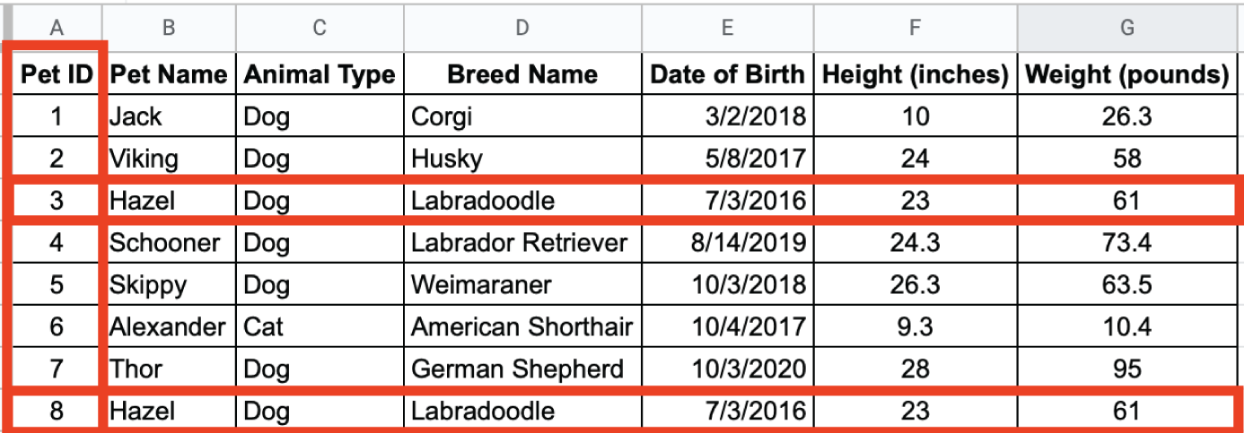
FIGURE 2.21 Pet ID as a key
Unstructured Data
Unstructured data is qualitative, describing characteristics about an event or an object. Images, phrases, audio or video recordings, and descriptive text are all examples of unstructured data. There is very little that is common about different kinds of unstructured data. Since the data is highly variable, its organizational and storage needs are different from structured data. Unstructured data also represents a significant opportunity. A Forbes study shows that over 90 percent of businesses need to manage and derive value from unstructured data.
Machine data is a common source of unstructured data. Machine data has various sources, including Internet of Things devices, smartphones, tablets, personal computers, and servers. As machines operate, they create digital footprints of their activity. This data is unstructured and can identify machine-to-machine interaction. Although some may think of machine data as digital exhaust, it is a treasure trove just waiting to be exploited by organizations.
A wide variety of technologies has emerged to facilitate the storage of unstructured data. Operationally, these technologies are similar to how a key in a tabular dataset identifies its associated values. With unstructured data, the key is a unique identifier, whereas the value is the unstructured data itself.
Consider the log entry shown in Figure 2.22. As an example of machine data, it represents a single entry within a log file generated when accessing a specific image on the Internet. The log entry contains a mix of seemingly random strings, time stamps, IP addresses, URLs, and browser metadata.

FIGURE 2.22 Unstructured data: log entry
Object storage facilitates the storage of unstructured data. The key-value concept underpins the design of object storage. The key is a unique identifier, and the value is the unstructured data itself. In Figure 2.23, the key is the filename, and the value is the contents of the file itself. Note that in this figure, each file is of a different type. The word document.docx is a Microsoft Word file, textfile.txt contains plain-text data, and the png image.png and lp_image-8.jpeg objects are digital images.
To access the contents of a file, you need to know its key. Figure 2.24 illustrates how an individual key serves as a reference to its unstructured data.

FIGURE 2.23 Files in object storage

FIGURE 2.24 Keys and values in object storage
Semi-structured Data
Semi-structured data is data that has structure and that is not tabular. Email is a well-known example of semi-structured data. Every email message has structural components, including recipient, sender, subject, date, and time. However, the body of an email is unstructured text, while attachments could be anything type of file.
The need to make semi-structured data easier to work with has led to the emergence of semi-structured formatting options. These formatting options use separators or tags to provide some context around a data element. Let's explore common file formats for transporting semi-structured data.
Common File Formats
Common file formats facilitate data exchange and tool interoperability. Several file formats have emerged as standards and are widely adopted. As a modern data analyst, you will need to recognize all of these formats and be familiar with common use cases for each type.
Text Files
Text files are one of the most commonly used data file formats. As the name implies, they consist of plain text and are limited in scope to alphanumeric data. One of the reasons text files are so widely adopted is their ability to be opened regardless of platform or operating system without needing a proprietary piece of software. Whether you are using a Microsoft Windows desktop, an Apple MacBook, or a Linux server, you can easily open a text file. Text files are also commonly referred to as flat files.
When machines generate data, the output is commonly stored in a text file. For example, the unstructured log entry, as illustrated in Figure 2.22, is an excerpt taken from a plain-text file.
A unique character known as a delimiter facilitates transmitting structured data via a text file. The delimiter is the character that separates individual fields. A delimiter can be any character. Over the years, the comma and tab grew into a widely accepted standard. Various software packages support reading and writing delimited files using the comma and the tab. In addition, many coding languages have libraries that make it easy to write comma- or tab-delimited files. When a file is comma-delimited, it is known as a comma-separated values (CSV) file. Similarly, when a file is tab-delimited, it is called a tab-separated values (TSV) file.
Suppose you have the pet data from Table 2.1 in a Google spreadsheet. Figure 2.25 illustrates how it is possible to download the data as either a comma- or tab-delimited file. Microsoft Excel also supports CSV and TSV as options.

FIGURE 2.25 Exporting as CSV or TSV
Note that the columns in Figure 2.26 do not line up with each other. The width of each column is variable, only as long as it needs to be to store the data in each row.

FIGURE 2.26 Contents of a CSV file
You may think that all CSV files represent structured data. Consider Figure 2.27, containing an excerpt from playback-related events from a Netflix viewer. Every column header except for Playtraces is structured. However, note the contents of the Playtraces field within the red rectangle. It contains quite a bit of text that appears to have a structure of its own.

FIGURE 2.27 Semi-structured CSV
JavaScript Object Notation
JavaScript Object Notation (JSON) is an open standard file format, designed to add structure to a text file without incurring significant overhead. One of its design principles is that JSON is easily readable by people and easily parsed by modern programming languages. Languages such as Python, R, and Go have libraries containing functions that facilitate reading and writing JSON files.
Consider Figure 2.29, which illustrates data about the first three pets from Table 2.1, formatted as JSON. As a person, it is easy to see that the information corresponding to an individual pet is within curly braces, with name-value pairs corresponding to the data elements and values.
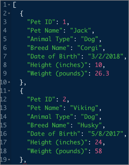
FIGURE 2.29 Pet data JSON example
To illustrate how a machine processes this same information, Figure 2.30 shows how the entire pet data, formatted as JSON, is read using the Python programming language. Figure 2.31 illustrates reading the same file using the R programming language. Note that R, which facilitates statistical analysis of data, has a summary command, the results of which illustrate some summary statistics about the pet data. The summary statistics are convenient, as it shows six dogs and only one cat in this dataset. It also shows the quartile breakdowns for height and weight.
Extensible Markup Language (XML)
Extensible Markup Language (XML) is a markup language that facilitates structuring data in a text file. While conceptually similar to JSON, XML incurs more overhead because it makes extensive use of tags. Tags describe a data element and enclose each value for each data element. While these tags help readability, they add a significant amount of overhead.
Consider Figure 2.32, which illustrates an XML representation for a single pet. Note that for each data element, there is an open tag that defines the element, followed by its value and a closing tag. Compared with the JSON in Figure 2.29, XML results in a file roughly double in size. Although this is insignificant for small files, the impact is much more profound when dealing with data in the gigabyte and terabyte range.

FIGURE 2.30 Reading JSON in Python
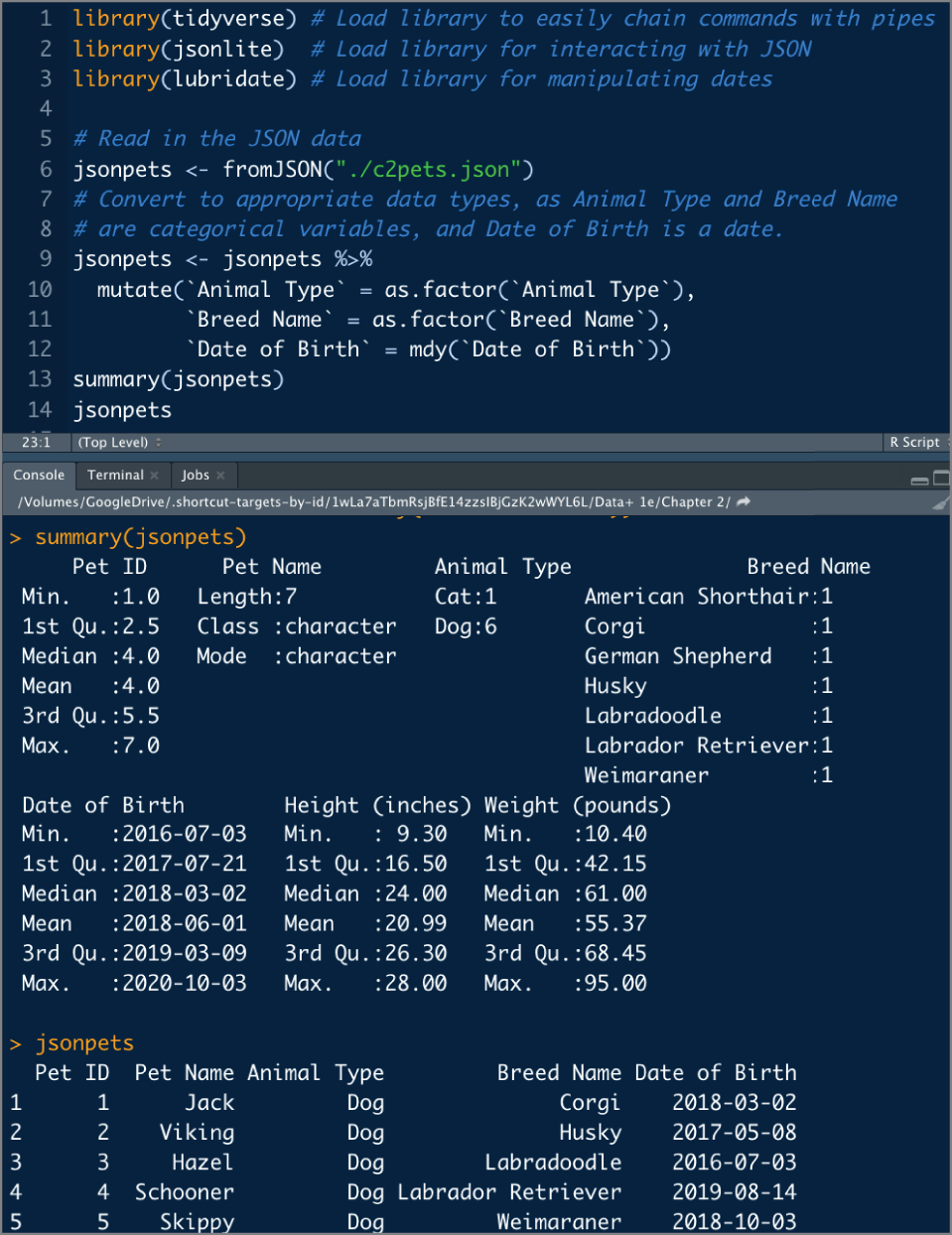
FIGURE 2.31 Reading JSON in R
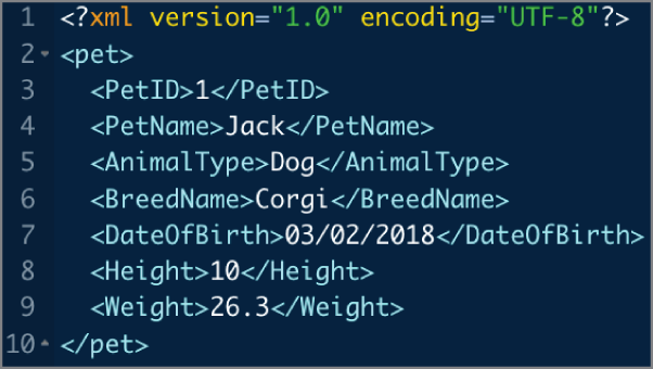
FIGURE 2.32 Representing a single animal in XML
In 1999, XML was the data format of choice and facilitated Asynchronous JavaScript and XML (Ajax) web development techniques. AJAX allowed client applications, written in HTML, to retrieve data from a server asynchronously. Without having to wait for a server response, the speed with which dynamic web pages operated increased. With JSON as a lighter-weight alternative to XML, it is becoming increasingly popular when interacting asynchronously between a web browser and a remote server.
HyperText Markup Language (HTML)
HyperText Markup Language (HTML) is a markup language for documents designed to be displayed in a web browser. HTML pages serve as the foundation for how people interact with the World Wide Web. Similar to XML, HTML is a tag-based language. Figure 2.33 illustrates the creation of a table in HTML containing the data for a single pet. Figure 2.34 illustrates how a browser processes an HTML of fully populated pet data to display it to people.
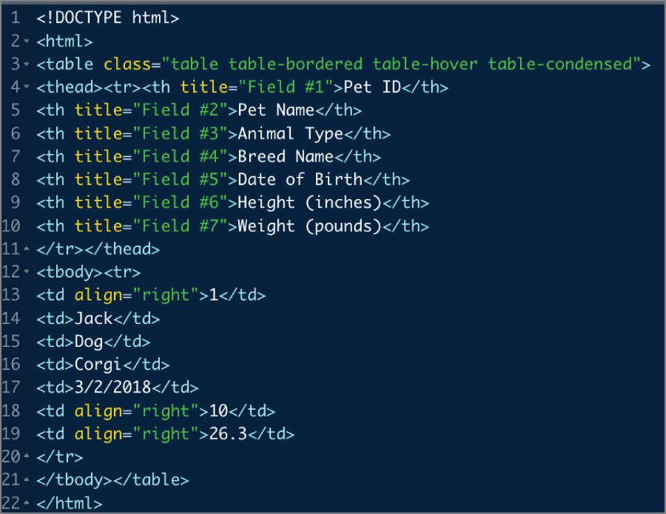
FIGURE 2.33 Representing a single animal in HTML

FIGURE 2.34 HTML table in a browser
Most people interact with HTML as interpreted by a web browser. HTML has become increasingly sophisticated over the years, with the ability for developers to create web pages that dynamically display content, adjust to different screen sizes, and play videos. Among the many tags that HTML supports is the image tag. It would be possible to display a picture for each pet in the table using image tags. Figure 2.35 illustrates the code that makes this happen.

FIGURE 2.35 Displaying an image in an HTML table
Summary
When dealing with data, you need to think through the data values you are working with, because doing so influences your choice of data type. When using structured data, you may be working with dates, numbers, text, currency, or alphanumeric data. Whether the data is discrete, continuous, or categorical, choosing the appropriate data type can help boost data quality. There are also data types for storing unstructured data, such as images, audio, and video.
If you are working with structured data, you should start thinking about it in a tabular fashion. Getting structured data into unique rows and consistent columns is the first step on the path to preparing data for analysis. Structured data fits well into CSV files, a popular format for exchanging data via flat files.
When you have to incorporate additional metadata or represent a complex data structure, you need capabilities beyond what a flat file provides. Formatting the data as JSON or XML is a viable alternative.
The modern analyst frequently works with data sources over the Internet. Understanding that HTML is the standard for structuring web pages is crucial to developing the ability to interact with data over the Internet programmatically.
Exam Essentials
Consider the values of what you will store before selecting data types. Data types are used to store different kinds of values. When dealing with numeric information, the best option is a numeric data type that can accommodate decimals. For sequences of whole numbers, an integer data type is a good choice. Be wary of using currency-specific data types—that can lead to calculation errors. For text values, the alphanumeric data type is the optimal choice. When dealing with dates, you will want to consider whether you need to store the time as well. For binary data, including audio, video, and images, you should use a BLOB data type.
Know that you can format data after storing it. While data types determine how data gets stored, formatting data governs how data will be displayed to a person. You may wish to store numeric data to many decimal places but round to the hundredths for display purposes. Similarly, numeric data can be formatted and displayed as a currency. Dates are possibly the most commonly formatted data type, since the same information may need to be displayed differently depending on cultural norms.
Consider the absolute limits of values that you will use before selecting data types. When selecting data types, consider the range of values that a data element can contain. Suppose the values need to fall within a given, defined range. In that case, you must select a data element that can support discrete data. If the data element's range is unknown, a data element that supports continuous data is necessary.
Explain the differences between structured and unstructured data. Individual data elements fall along the structured data continuum. At one end, there is highly structured, rectangular data. Structured data is organized into columns and rows. Each column has a consistent data type, and each row contains data about one data subject. Unstructured data does not fit neatly into a column. Looking for similarities or differences in unstructured data requires more advanced analytical techniques than structured data.
Understand the differences in common file formats. Common file formats make it easy for people to read a file's contents and facilitate interoperability between tools. Delimiters separate variable-length fields in a file. The comma and the resultant CSV file are among the most commonly used formats for exchanging text files. To provide additional metadata about data values and support more complex data structures, XML and JSON were developed. JSON is a preferred format, given its low overhead, especially when compared with XML.
Review Questions
- Enzo is building a database that will store flight information for his travel agency. He is adding a field to a table that will contain flight numbers. A flight number is a combination of a two-character airline designator and a one-to-four-digit number. For example, United Airlines flight 769 between Chicago and San Francisco has flight number UA 769. What data type would be most appropriate for this field?
- Date
- Numeric
- Text
- Alphanumeric
- Madeline is building a medical transcription system, which transcribes physician voice reports so they can be easily read by other healthcare professionals. Which of the following data types is the most appropriate for her to select in order to store the raw recordings?
- Alphanumeric
- Numeric
- BLOB
- Date
- Rupert is working on implementing a general ledger system that can accommodate financial records in excess of $1 million. Which of the following data types is the most appropriate for him to select in order to store financial transactions?
- Alphanumeric
- Smallmoney
- Money
- Numeric
- Hazel needs to store video recordings for subjects participating in a psychological experiment. There are 300 participants in the experiment, and each session is 45 minutes long. Presuming the video is captured using a modern smartphone at a rate of 102,400 KB per minute, which of the following data types does Hazel need to select if she is storing these videos in a database?
- Varbinary
- BLOB
- CLOB
- Numeric
- Alexander is doing research on literary works and wants to store the title, complete text, and community-sourced rating in a database. The longest book included in his study is Atlas Shrugged by Ayn Rand, coming in at 1,168 pages. Presuming that Alexander is working in an Oracle database, which of the following data types should he choose?
- BLOB
- CLOB
- varchar
- Numeric
- Barnali is analyzing defects at a manufacturing plant. In order to inform her work, she tracks the number of defective control arms that come down the assembly line on an hourly basis. What kind of data is represented by the number of defects?
- Discrete
- Continuous
- Categorical
- Alphanumeric
- Haroon is choosing a pair of running shoes. In the past, he has found a size 10 to be too small and size 10.5 to be uncomfortable. While he would like to be able to order a size 10.25, it is simply not available as shoes are sold in half-size increments. What kind of data is represented by shoe size?
- Discrete
- Continuous
- Categorical
- Alphanumeric
- Amdee is measuring her feet to help her figure out what shoe size to order. At 9.75 inches, that places her between a U.S. size 8 and a U.S. size 8.5 shoe. What kind of data does Amdee's measured foot size represent?
- Discrete
- Continuous
- Categorical
- Alphanumeric
- Connor is aggregating temperature information from 5,000 Internet of Things temperature sensors at disparate locations around his farm. What type of measure is temperature, and what is an appropriate data type to contain these values?
- Discrete; integer
- Discrete; numeric
- Continuous; integer
- Continuous; numeric
- Zahara is conducting a survey to collect opinions about a recent theatrical release. She is capturing this via an open-ended text response field on a web form. What category of data does this represent?
- Quantitative
- Qualitative
- Categorical
- Dimensional
- Jed wants to track his expenditures in a spreadsheet containing check number, date, recipient, and amount. What kind of data is Jed working with?
- Unstructured
- Semi-structured
- Structured
- Machine
- Amy is interested in exploring the Netflix viewing history, including Profile Name, Title Description, Device, Country, Playback Start Times, and Playtraces, for her household. Navigating to the account export screen, which option should she select in order to facilitate analysis using the Python programming language?
- CSV
- Text file
- HTML
- XML
- Zeke is experimenting with home automation. Reading the application programming interface (API) guide, he sees that commands can be issued in the following syntax:
{"commands": [{"component": "main","capability": "switch","command": "off","arguments": []}]}Which data format does the API require?
- JSON
- TSV
- CSV
- XML
- Maura is a data engineer tasked with a new system integration. She has been given the following sample file to help her understand how to parse files of a similar type:
{"VIN": "WP0ZZZ99Z5S73824","Manufacturer": "Porsche","Model": "Carrera S","Horsepower": "443","Torque": "390"}Which data format does the API require?
- JSON
- TSV
- CSV
- XML
- Chris is a financial analyst who wants to use Microsoft Excel to perform what-if analysis on data extracted from his corporate accounting system. To make the data extract easy to import, which of the following file formats should he specify?
- CSV
- JSON
- XML
- YAML
- Claire is a web developer working on an interactive website. While she is programming in JavaScript, which of the following file types is essential to test her work in a web browser?
- CSV
- JSON
- HTML
- XML
- Claire has just received a spreadsheet of streaming media use data, and one of the columns contained the following data:
[{"eventType":"start","sessionOffsetMs":0,"mediaOffsetMs":0},{"eventType":"playing","sessionOffsetMs":3153,"mediaOffsetMs":0},{"eventType":"stopped","sessionOffsetMs":4818,"mediaOffsetMs":559}]While the spreadsheet is displaying this data as a single piece of text, Claire feels like there is structure to the data. Is Claire correct, and if so, how are the contents of the column formatted?
- No; it is plain text.
- No; it is machine data.
- Yes; it is JSON.
- Yes; it is plain text.
- Jorge is transferring data from a mainframe to his laptop so that he can upload it into a Google spreadsheet for analysis. Looking at the file from the mainframe, he sees that it uses
^%as a delimiter. In order to make it easy to load into the Google spreadsheet, what should Jorge do?- Nothing, the file will load just fine.
- Nothing, you cannot transfer data from a mainframe to a laptop.
- Use software on the mainframe instead of a Google spreadsheet.
- Convert the
^%into a comma or a tab.
- Eleanora has been tasked with analyzing web server logs to better understand where website visitors are coming from. Every time a person visits a website, an entry containing multiple items, including IP address, destination page, and current time, is automatically made in the log. What type of data is this?
- Machine data
- Undefined data
- Automatic data
- Web data
- Dave is a graphic designer who wants to build a website to show off his portfolio. For each item in his portfolio, he wants to show the client name, date of commission, and a thumbnail image of the artwork. While he can accomplish this by building out a table in HTML, what category of data best describes what he wants to do?
- Unstructured
- Semi-structured
- Structured
- Machine